Available Software

Service:

Fields of Science:

BLAST Database

OSC periodically updates The NCBI BLAST database.

Versions

BLAST database is available on the Owens and Pitzer clusters. The versions currently available at OSC are:

Version	Owens	Pitzer
2017-03	X
2017-10	X*
2018-08	X	X*
2019-09	X	X
2020-04	X	X

* Current default version

The version indicates the date of download. You can usemodule spider blast-database to view available modules for a given machine. Feel free to contact OSC Help if you need other versions for your work.

Access

BLAST database is available to all OSC users. If you have any questions, please contact OSC Help.

Usage

BLAST database can be accessed with the following module:

module load blast-database/version

To list all the BLAST database available

module spider blast-database

BLAST database can be accessed by the environmental variable BLASTDB. For blast-database/2018-08, it is as follows

BLASTDB=/fs/project/pub_data/blast-database/2018-08

Microbial Genomes Database

Microbial Genomes is a database of prokaryotic genome sequencing project data.

Availability and Restrictions

Versions

Microbial Genomes is available on the Owens cluster. The versions currently available at OSC are:

Version	Owens
2017-11	X*

* Current default version

The version indicates the date of the installation. You can use module spider microbial-database to view available modules for a given machine. Feel free to contact OSC Help if you need other versions for your work.

Access

Microbial Genomes is available to all OSC users. If you have any questions, please contact OSC Help.

Usage

Usage on Owens

Set-up

To configure your enviorment for use of TrimGalore, use command module load microbial-database. This will load the default version.

The database can be accessed by the environment variable MICROBIALDB, for example

 >> ls $MICROBIALDB
Archaea_Genome  Bacteria_Genome  Fungi_Genome  Protozoa_Genome  Virus_Genome

Software Forms

Several of our software packages require that users complete a form that is then kept on record here before we can grant access to the software. OSC will provide you with the proper forms and instructions; please contact OSC Help noting which software package(s) you would like access.

The following list includes third-party software packages that require additional forms be completed:

ABAQUS

Amber

ANSYS

CASINO

CNS

CSD

FLUENT

GATK

Gaussian

Hyperworks

MATLAB DCS

MuTect

SIESTA

STAR-CCM+

Turbomole

Requesting additional software

If you would like to request that the center install (and purchase, if necessary) software, please complete the Request for Software Form. The return instructions are noted on the form.

If you have licensed software and you need assistance installing the software and restricting it's use to your group, please contact OSC Help.

Service:

Software List

Ohio Supercomputer Center (OSC) has a variety of software applications to support all aspects of scientific research. We are actively updating this documentation to ensure it matches the state of the supercomputers. This page is currently missing some content; use module spider on each system for a comprehensive list of available software.

Supercomputer:

Service:

ABAQUS

ABAQUS is a finite element analysis program owned and supported by SIMULIA, the Dassault Systèmes brand for Realistic Simulation.

Availability and Restrictions

Versions

The available programs are ABAQUS/CAE, ABAQUS/Standard and ABAQUS/Explicit. The versions currently available at OSC are:

Version	Owens	Notes
6.13
6.14	X
2016	X	Version scheme has been changed
2017	X
2018	X
2020	X*

*: Default Version

You can use module spider abaqus to view available modules for a given machine. Feel free to contact OSC Help if you need other versions for your work.

Access for Academic Users

OSC's ABAQUS license can only be used for educational, institutional, instructional, and/or research purposes. Only users who are faculty, research staff or students at the following institutions are permitted to utilized OSC's license:

The Ohio State University
University of Toledo
University of Cincinnati
University of Dayton
University of Akron

Users from additional degree granting academic institutions may request to be added to this list per a cost by contacting OSC Help.

The use of ABAQUS for academic purposes requires validation. In order to obtain validation, please contact OSC Help for further instruction.

(link sends e-mail)

Access for Commerical Users

Contact OSC Help for getting access to SOFTWARE if you are a commerical user.

Publisher/Vendor/Repository and License Type

Dassault Systemes, Commercial

Usage

Token Usage

ABAQUS software usage is monitored though a token-based license manager. This means every time you run a ABAQUS job, tokens are checked out from our pool for your tasks usage. To ensure your job is only started when its required ABAQUS tokens are available it is important to include a software flag within your job script's SBATCH directives. A minimum of 5 tokens are required per a job, so a 1 node, 1 processor ABAQUS job would need the following SBATCH software flag: #SBATCH -L abaqus@osc:5 . Jobs requiring more cores will need to request more tokens as calculated with the formula: M = int(5 x N^0.422) , where N is the total number of cores. For common requests, you can refer to the following table:

Cores (nodes x ppn each):	1	2	3	4	6	8	12	16	28	32	56
Tokens needed:	5	6	7	8	10	12	14	16	20	21	27

Usage on Owens

Set-up on Owens

To load the default version of ABAQUS module, use module load abaqus . To select a particular software version, use module load abaqus/version . For example, use module load abaqus/2016 to load ABAQUS version 2016 on Owens.

Using ABAQUS

Example input data files are available with the ABAQUS release. The abaqus fetch utility is used to extract these input files for use. For example, to fetch input file for one of the sample problems including 4 input files, type:

abaqus fetch job=knee_bolster

abaqus fetch job=knee_bolster_ef1

abaqus fetch job=knee_bolster_ef2

abaqus fetch job=knee_bolster_ef3

Also, use the abaqus help utility is to list all the abaqus execution procedures.

Batch Usage on Owens

Interactive Batch Session

For an interactive batch session on Owens, one can run the following command:

sinteractive -A <project-account> -N 1 -n 28 -t 1:00:00 -L abaqus@osc:20

which gives you 28 cores ( -N 1 -n 28 ) with 1 hour ( -t 1:00:00 ). You may adjust the numbers per your need.

Non-interactive Batch Job (Serial Run)

A batch script can be created and submitted for a serial or parallel run. You can create the batch script using any text editor you like in a working directory on the system of your choice.

Below is the example batch script ( job.txt ) for a serial run:

#!/bin/bash
#SBATCH --time=1:00:00
#SBATCH --nodes=1 --ntasks-per-node=1
#SBATCH -L abaqus@osc:5
#SBATCH --account=<project-account>
#
# The following lines set up the ABAQUS environment
#
module load abaqus
#
cp *.inp $TMPDIR
cd $TMPDIR
#
# Run ABAQUS
#
abaqus job=knee_bolster interactive
#
# Now, copy data (or move) back once the simulation has completed
#
cp * $SLURM_SUBMIT_DIR

In order to run it via the batch system, submit the job.txt file with the command: qsub job.txt

NOTE:

Make sure to copy all the files needed (input files, restart files, user subroutines, python scripts etc.) from your work directory ( $SLURM_SUBMIT_DIR ) to $TMPDIR , and copy your results back at the end of your script. Running your job on $TMPDIR ensures maximum efficiency.
The keyword interactive is required in the execution line abaqus job=knee_bolster interactive for the following reason: If left off, ABAQUS will background the simulation process. Backgrounding a process in the OSC environment will place it outside of the batch job and it will receive the default 1 hour of CPU time and corresponding default memory limits. The keyword interactive in this case simply tells ABAQUS not to return until the simulation has completed.
The name of the input file is sometimes omitted in the execution line, which may work fine if you've copied only the input files for one specific model. Although, it is better practice to designate the main input file explicitly by adding input=<my_input_file_name>.inp to the execution line so that it looks like abaqus job=knee_bolster input=<my_input_file_name>.inp interactive .
Define nodes=1 (1<=ppn<=28 for Owens) for a serial run.
If ppn>1, add cpus=<n> to the execution line, where n=ppn. This is how it should look like: abaqus job=test input=<my_input_file_name1>.inp cpus=<n> interactive .

Non-interactive Batch Job (Parallel Run)

Note: abaqus will not run correctly in parallel with input files in $TMPDIR! Use the scratch file system.

Below is the example batch script ( job.txt ) for a parallel run:

#!/bin/bash 
#SBATCH --time=1:00:00 
#SBATCH --nodes=2 --ntasks-per-node=28 --gres=pfsdir
#SBATCH -L abaqus@osc:27
#SBATCH --account=<project-account>
#
# The following lines set up the ABAQUS environment
#
module load abaqus
#
# Cope input files to /fs/scratch and run Abaqus there
#
cp *.inp $PFSDIR
cd $PFSDIR
#
# Run ABAQUS, note that in this case we have provided the names of the input files explicitly
#
abaqus job=test input=<my_input_file_name1>.inp cpus=$SLURM_NTASKS interactive
#
# Now, move data back once the simulation has completed
#
mv * $SLURM_SUBMIT_DIR

NOTE:

If you request a partial node for a serial job (nodes=1:ppn<28), you need to add 'mp_mode=threads' option in order to get the full performance.
Specify cpus=<n> in the execution line, where n=nodes*ppn.
Everything else is similar to the serial script above.
Usage of user-defined material (UMAT) script in Fortran is limited on Owens as following:
1. abaqus 2017: correctly running on single and multi-nodes
2. abaqus 6.14 and 2016: correctly running on a single node

AMBER

The Assisted Model Building with Energy Refinement (AMBER) package contains many molecular simulation programs targeted at biomolecular systems. A wide variety of modelling techniques are available. It generally scales well on modest numbers of processors, and the GPU enabled CUDA programs are very efficient.

Availability and Restrictions

Versions

AMBER is available on Owens and Pitzer Clusters. The following versions are currently available at OSC (S means serial executables, P means parallel, C means CUDA, i.e., GPU enabled, and M means MIC, i.e., Xeon Phi enabled):

Version	Owens	Pitzer
18	SPC	SPC
19	SPC*	SPC*
20	SPC	SPC

* Current default version

* IMPORTANT NOTE: You need to load correct compiler and MPI modules before you use Amber. In order to find out what modules you need, use module spider amber/{version} .

You can use module spider amber to view available modules for a given machine. Feel free to contact OSC Help if you need other versions for your work.

Access for Academic Users

OSC's Amber is available to not-for-profit OSC users; simply contact OSC Help to request the appropriate form for access.

Access for Commerical Users

For-profit OSC users must obtain their own Amber license.

Publisher/Vendor/Repository and License Type

University of California, San Francisco, Commercial

Usage

Usage on Owens

Set-up

To load the default version of AMBER module, use module load amber . To select a particular software version, use module load amber/version . For example, use module load amber/16 to load AMBER version 16.

Using AMBER

A serial Amber program in a short duration run can be executed interactively on the command line, e.g.:

tleap

Parallel Amber programs must be run in a batch environment with srun, e.g.:

srun pmemd.MPI

Batch Usage

Interactive Batch Session

For an interactive batch session, one can run the following command:

sinteractive -A <project-account> -N 1 -n 28 -t 1:00:00

which gives you one node with 28 cores ( -N 1 -n 28 ), with 1 hour ( -t 1:00:00 ). You may adjust the numbers per your need.

Non-interactive Batch Job (Serial Run)

~srb/workshops/compchem/amber/

Below is the example batch script ( job.txt ) for a serial run:

# AMBER Example Batch Script for the Basic Tutorial in the Amber manual
#!/bin/bash
#SBATCH --job-name 6pti
#SBATCH --nodes=1 --ntasks-per-node=28
#SBATCH --time=0:20:00
#SBATCH --account=<project-account>

module load amber
# Use TMPDIR for best performance.
cd $TMPDIR
# SLURM_SUBMIT_DIR refers to the directory from which the job was submitted.
cp -p $SLURM_SUBMIT_DIR/6pti.prmtop .
cp -p $SLURM_SUBMIT_DIR/6pti.prmcrd .
# Running minimization for BPTI
cat << eof > min.in
# 200 steps of minimization, generalized Born solvent model
&cntrl
maxcyc=200, imin=1, cut=12.0, igb=1, ntb=0, ntpr=10,
/
eof
sander -i min.in -o 6pti.min1.out -p 6pti.prmtop -c 6pti.prmcrd -r 6pti.min1.xyz
cp -p min.in 6pti.min1.out 6pti.min1.xyz $SLURM_SUBMIT_DIR

In order to run it via the batch system, submit the job.txt file with the command: sbatch job.txt .

Usage on Pitzer

Set-up

To load the default version of AMBER module, use module load amber.

Using AMBER

A serial Amber program in a short duration run can be executed interactively on the command line, e.g.:

tleap

Parallel Amber programs must be run in a batch environment with mpiexec, e.g.:

srun pmemd.MPI

Batch Usage

Interactive Batch Session

For an interactive batch session, one can run the following command:

sinteractive -A <project-account> -N 1 -n 48 -t 1:00:00

which gives you one node with 48 cores ( -N 1 -n 48) with 1 hour ( -t 1:00:00). You may adjust the numbers per your need.

Non-interactive Batch Job (Serial Run)

~srb/workshops/compchem/amber/

Below is the example batch script ( job.txt ) for a serial run:

# AMBER Example Batch Script for the Basic Tutorial in the Amber manual 
#!/bin/bash
#SBATCH --job-name 6pti #
SBATCH --nodes=1 --ntasks-per-node=48 
SBATCH --time=0:20:00
#SBATCH --account=<project-account>

module load amber
# Use TMPDIR for best performance.
cd $TMPDIR
# SLURM_SUBMIT_DIR refers to the directory from which the job was submitted.
cp -p $SLURM_SUBMIT_DIR/6pti.prmtop .
cp -p $SLURM_SUBMIT_DIR/6pti.prmcrd .
# Running minimization for BPTI
cat << eof > min.in
# 200 steps of minimization, generalized Born solvent model
&cntrl
maxcyc=200, imin=1, cut=12.0, igb=1, ntb=0, ntpr=10,
/
eof
sander -i min.in -o 6pti.min1.out -p 6pti.prmtop -c 6pti.prmcrd -r 6pti.min1.xyz
cp -p min.in 6pti.min1.out 6pti.min1.xyz $SLURM_SUBMIT_DIR

In order to run it via the batch system, submit the job.txt file with the command: sbatch job.txt .

Troubleshooting

In general, the scientific method should be applied to usage problems. Users should check all inputs and examine all outputs for the first signs of trouble. When one cannot find issues with ones inputs, it is often helpful to ask fellow humans, especially labmates, to review the inputs and outputs. Reproducibility of molecular dynamics simulations is subject to many caveats. See page 24 of the Amber18 manual for a discussion.

ANSYS

ANSYS offers a comprehensive software suite that spans the entire range of physics, providing access to virtually any field of engineering simulation that a design process requires. Supports are provided by ANSYS, Inc.

Availability and Restrictions

Versions

Version	Owens
17.2	X
18.1	X
19.1	X
19.2	X
2019R1	X
2019R2	X
2020R1	X*
2020R2	X
2021R1	X

* Current default version

OSC has Academic Multiphysics Campus Solution license from Ansys. The license includes most of all the features that Ansys provides. See "Academic Multiphyscis Campus Solution Products" in this table for all available products at OSC.

Access for Academic Users

OSC has an "Academic Research " license for ANSYS. This allows for academic use of the software by Ohio faculty and students, with some restrictions. To view current ANSYS node restrictions, please see ANSYS's Terms of Use.

Use of ANSYS products at OSC for academic purposes requires validation. Please contact OSC Help for further instruction.

Access for Commerical Users

Contact OSC Help for getting access to ANSYS if you are a commercial user.

Publisher/Vendor/Repository and License Type

Ansys, Inc., Commercial

Usage

For more information on how to use each ANSYS product at OSC systems, refer to its documentation page provided at the end of this page.

Note

Due to the way our Fluent and ANSYS modules are configured, simultaneously loading multiple of either module will cause a cryptic error. The most common case of this happening is when multiple of a user's jobs are started at the same time and all load the module at once. In order for this error to manifest, the modules have to be loaded at precisely the same time; a rare occurrence, but a probable occurrence over the long term.

If you encounter this error you are not at fault. Please resubmit the failed job(s).

If you frequently submit large amounts of Fluent or ANSYS jobs, we recommend you stagger your job submit times to lower the chances of two jobs starting at the same time, and hence loading the module at the same time. Another solution is to establish job dependencies between jobs, so jobs will only start one after another. To do this, you would add the SLURM directive:

#SBATCH --dependency=after:jobid

To jobs you want to only start after another job has started. You would replace jobid with the job ID of the job to wait for. If you have additional questions, please contact OSC Help.

ANSYS Mechanical

ANSYS Mechanical is a finite element analysis (FEA) tool that enables you to analyze complex product architectures and solve difficult mechanical problems. You can use ANSYS Mechanical to simulate real world behavior of components and sub-systems, and customize it to test design variations quickly and accurately.

Availability and Restrictions

ANSYS Mechanical is available on the Owens Cluster. The versions currently available at OSC are:

Version	owens
17.2	X
18.1	X
19.1	X
19.2	X
2019R1	X
2019R2	X
2020R1	X*
2020R2	X
2021R1	X

* Current default version

You can use module spider ansys to view available modules for a given machine. Feel free to contact OSC Help if you need other versions for your work.

Access for Academic Users

Use of ANSYS for academic purposes requires validation. In order to obtain validation, please contact OSC Help for further instruction.

Access for Commerical Users

Contact OSC Help for getting access to ANSYS if you are a commerical user.

Usage

Usage on Owens

Set-up on Owens

To load the default version of ANSYS module, use module load ansys . To select a particular software version, use module load ansys/version . For example, use module load ansys/17.2 to load ANSYS version 17.2 on Owens.

Using ANSYS Mechanical

Following a successful loading of the ANSYS module, you can access the ANSYS Mechanical commands and utility programs located in your execution path:

ansys <switch options> <file>

The ANSYS Mechanical command takes a number of Unix-style switches and parameters.

The -j Switch

The command accepts a -j switch. It specifies the "job id," which determines the naming of output files. The default is the name of the input file.

The -d Switch

The command accepts a -d switch. It specifies the device type. The value can be X11, x11, X11C, x11c, or 3D.

The -m Switch

The command accepts a -m switch. It specifies the amount of working storage obtained from the system. The units are megawords.

The memory requirement for the entire execution will be approximately 5300000 words more than the -m specification. This is calculated for you if you use ansnqs to construct an NQS request.

The -b [nolist] Switch

The command accepts a -b switch. It specifies that no user input is expected (batch execution).

The -s [noread] Switch

The command accepts a -s switch. By default, the start-up file is read during an interactive session and not read during batch execution. These defaults may be changed with the -s command line argument. The noread option of the -s argument specifies that the start-up file is not to be read, even during an interactive session. Conversely, the -s argument with the -b batch argument forces the reading of the start-up file during batch execution.

The -g [off] Switch

The command accepts a -g switch. It specifies that the ANSYS graphical user interface started automatically.

ANSYS Mechanical parameters

ANSYS Mechanical parameters may be assigned values on the command. The parameter must be at least two characters long and must be a legal parameter name. The ANSYS Mechanical parameter that is to be assigned a value should be given on the command line with a preceding dash (-), a space immediately after, and the value immediately after the space:

module load ansys
ansys -pval1 -10.2 -EEE .1e6
sets pval1 to -10.2 and EEE to 100000

Batch Usage on Owens

When you log into owens.osc.edu you are actually logged into a linux box referred to as the login node. To gain access to the mutiple processors in the computing environment, you must submit your ANSYS Mechanical analysis to the batch system for execution. Batch jobs can request mutiple nodes/cores and compute time up to the limits of the OSC systems. Refer to Queues and Reservations and Batch Limit Rules for more info. Batch jobs run on the compute nodes of the system and not on the login node. It is desirable for big problems since more resources can be used.

Interactive Batch Session

Interactive mode is similar to running ANSYS Mechanical on a desktop machine in that the graphical user interface will be sent from OSC and displayed on the local machine. Interactive jobs are run on compute nodes of the cluster, by turning on X11 forwarding. The intention is that users can run ANSYS Mechanical interactively for the purpose of building their model and preparing their input file. Once developed this input file can then be run in no-interactive batch mode.

To run interactive ANSYS Mechanical, a batch job need to be submitted from the login node, to request necessary compute resources, with X11 forwarding. For example, the following command requests one whole node with 28 cores ( -N 1 -n 28 ), for a walltime of 1 hour ( -t 1:00:00 ), with one ANSYS license:

sinteractive -N 1 -n 28 -t 1:00:00 -L ansys@osc:1,ansyspar@osc:24 -A <account>

You may adjust the numbers per your need. This job will queue until resources becomes available. Once the job is started, you're automatically logged in on the compute node; and you can launch ANSYS Mechanical and start the graphic interface with the following commands:

module load ansys
ansys -g

Non-interactive Batch Job (Serial Run)

A batch script can be created and submitted for a serial or parallel run. You can create the batch script using any text editor you like in a working directory on the system of your choice. For a given model, prepare the input file with ANSYS Mechanical commands (named ansys.in for example) for the batch run. Below is the example batch script ( job.txt ) for a serial run:

#!/bin/bash
#SBATCH --job-name=ansys_test
#SBATCH --time=1:00:00
#SBATCH --nodes=1 --ntasks-per-node=1
#SBATCH -L ansys@osc:1
#SBATCH --account=<account>

cd $TMPDIR  
cp $SLURM_SUBMIT_DIR/ansys.in .    
module load ansys  
ansys < ansys.in   
cp <output files> $SLURM_SUBMIT_DIR

In order to run it via the batch system, submit the job.txt file with the command: qsub job.txt .

Non-interactive Batch Job (Parallel Run)

To take advantage of the powerful compute resources at OSC, you may choose to run distributed ANSYS Mechanical for large problems. Multiple nodes and cores can be requested to accelerate the solution time. Note that you'll need to change your batch script slightly for distributed runs.

Starting from September 15, 2015, a job using HPC tokens (with "ansyspar" flag) should be submitted to Owens clusters due to scheduler issue.

For distributed ANSYS Mechanical jobs, the number of processors needs to be specified in the command line with options '-dis -np':

#!/bin/bash
#SBATCH --job-name=ansys_test
#SBATCH --time=1:00:00
#SBATCH --nodes=1 --ntasks-per-node=28
#SBATCH --account=<account>
#SBATCH -L ansys@osc:1,ansyspar@osc:24

...
ansys -b -dis -mpi ibmmpi -np ${SLURM_NTASKS} -i ansys.in
 
...

Notice that in the script above, the ansys parallel license is requested as well as ansys license in the format of

#SBATCH -L ansys@osc:1,ansyspar@osc:n

where n=m-4, with m being the total cpus called for this job. This part is necessary when the total cpus called is greater than 4 (m>4), which applies for the parallel example below as well.

The following shows changes in the batch script if 2 nodes on Owens are requested for a parallel ANSYS Mechanical job:

#!/bin/bash
#SBATCH --job-name=ansys_test
#SBATCH --time=3:00:00
#SBATCH --nodes=2 --ntasks-per-node=28
#SBATCH -L ansys@osc:1,ansyspar@osc:52

...
ansys -b -dis -mpi ibmmpi -np ${SLURM_NTASKS} -i ansys.in 
...
pbsdcp -g '<output files>' $SLURM_SUBMIT_DIR

The 'pbsdcp -g' command in the last line in the script above makes sure that all result files generated by different compute nodes are copied back to the work directory.

CFX

ANSYS CFX (called CFX hereafter) is a computational fluid dynamics (CFD) program for modeling fluid flow and heat transfer in a variety of applications.

Availability and Restrictions

CFX is available on the Owens Cluster. The versions currently available at OSC are:

VERSION	owens
17.2	X
18.1	X
19.1	X*

* Current default version

You can use module spider fluent to view available modules for a given machine. Feel free to contact OSC Help if you need other versions for your work.

Access for Academic Users

Use of ANSYS products for academic purposes requires validation. In order to obtain validation, please contact OSC Help for further instruction.

Currently, there are in total 50 ANSYS base license tokens and 900 HPC tokens for academic users. These base tokens and HPC tokens are shared with all ANSYS products we have at OSC. A base license token will allow CFX to use up to 4 cores without any additional tokens. If you want to use more than 4 cores, you will need an additional "HPC" token per core. For instance, a serial CFX job with 1 core will need 1 base license token while a parallel CFX job with 28 cores will need 1 base license token and 24 HPC tokens.

Access for Commerical Users

Contact OSC Help for getting access to CFX if you are a commerical user.

Usage

Usage on Owens

Set-up on Owens

To load the default version, use module load ansys . To select a particular software version, use module load ansys/version . For example, use module load ansys/17.2 to load CFX version 17.2 on Owens.

Batch Usage on owens

When you log into owens.osc.edu you are actually logged into a linux box referred to as the login node. To gain access to the mutiple processors in the computing environment, you must submit your analysis to the batch system for execution. Batch jobs can request mutiple nodes/cores and compute time up to the limits of the OSC systems. Refer to Queues and Reservations and Batch Limit Rules for more info. Batch jobs run on the compute nodes of the system and not on the login node. It is desirable for big problems since more resources can be used.

Interactive Batch Session

Interactive mode is similar to running CFX on a desktop machine in that the graphical user interface will be sent from OSC and displayed on the local machine. Interactive jobs are run on compute nodes of the cluster, by turning on X11 forwarding. The intention is that users can run CFX interactively for the purpose of building their model and preparing their input file. Once developed this input file can then be run in no-interactive batch mode.

To run interactive CFX GUI, a batch job need to be submitted from the login node, to request necessary compute resources, with X11 forwarding. Please follwoing the steps below to use CFX GUI interactivly:

Ensure that your SSH client software has X11 forwarding enabled
Connect to Owens system
Request an interactive job. The command below will request one whole node with 28 cores ( -N 1 -n 28 ), for a walltime of one hour ( -t 1:00:00 ), with one ANSYS CFD license (modify as per your own needs):
```
sinteractive -N 1 -n 28 -t 1:00:00 -L ansys@osc:1,ansyspar@osc:24
```
Once the interactive job has started, run the following commands to setup and start the CFX GUI:
```
module load ansys
cfx5 
```

Non-interactive Batch Job (Serial Run Using 1 Base Token)

A batch script can be created and submitted for a serial or parallel run. You can create the batch script using any text editor you like in a working directory on the system of your choice.

Below is the example batch script ( job.txt ) for a serial run with an input file test.def ) :

#!/bin/bash
#SBATCH --job-name=serialjob_cfx
#SBATCH --time=1:00:00
#SBATCH --nodes=1 --ntasks-per-node=1
#SBATCH -L ansys@osc:1

#Set up CFX environment.
module load ansys
#Copy CFX files like .def to $TMPDIR and move there to execute the program
cp test.def $TMPDIR/
cd $TMPDIR
#Run CFX in serial with test.def as input file
cfx5solve -batch -def test.def 
#Finally, copy files back to your home directory
cp  * $SLURM_SUBMIT_DIR

In order to run it via the batch system, submit the job.txt file with the command: sbatch job.txt

Non-interactive Batch Job (Parallel Execution using HPC token)

CFX can be run in parallel, but it is very important that you read the documentation in the CFX Manual on the details of how this works.

In addition to requesting the base license token ( -L ansys@osc:1 ), you need to request copies of the ansyspar license, i.e., HPC tokens ( -L ansys@osc:1,ansyspar@osc:[n] ), where [n] is equal to the number of cores you requested minus 4.

Parallel jobs have to be submitted on Owens via the batch system. An example of the batch script follows:

#!/bin/bash
#SBATCH --job-name=paralleljob_cfx
#SBATCH --time=10:00:00
#SBATCH --nodes=2 --ntasks-per-node=28
#SBATCH -L ansys@osc:1,ansyspar@osc:52

#Set up CFX environment.
module load ansys
#Copy CFX files like .def to $TMPDIR and move there to execute the program
cp test.def $TMPDIR/
cd $TMPDIR
#Convert PBS_NODEFILE information into format for CFX host list
nodes=`cat $PBS_NODEFILE`
nodes=`echo $nodes | sed -e 's/ /,/g'`
#Run CFX in parallel with new.def as input file
#if multiple nodes
cfx5solve -batch -def test.def  -par-dist $nodes -start-method "Platform MPI Distributed Parallel"
#if one node
#cfx5solve -batch -def test.def -par-dist $nodes -start-method "Platform MPI Local Parallel"
#Finally, copy files back to your home directory
cp  * $SLURM_SUBMIT_DIR

FLUENT

ANSYS FLUENT (called FLUENT hereafter) is a state-of-the-art computer program for modeling fluid flow and heat transfer in complex geometries.

Availability and Restrictions

FLUENT is available on the Owens Cluster. The versions currently available at OSC are:

Version	owens
17.2	X
18.1	X
19.1	X*

* Current default version

You can use module spider ansy for Owens to view available modules for a given machine. Feel free to contact OSC Help if you need other versions for your work.

Access for Academic Users

Use of ANSYS products for academic purposes requires validation. In order to obtain validation, please contact OSC Help for further instruction.

Currently, there are in total 50 ANSYS base license tokens and 900 HPC tokens for academic users. These base tokens and HPC tokens are shared with all ANSYS products we have at OSC. A base license token will allow FLUENT to use up to 4 cores without any additional tokens. If you want to use more than 4 cores, you will need an additional "HPC" token per core. For instance, a serial FLUENT job with 1 core will need 1 base license token while a parallel FLUENT job with 28 cores will need 1 base license token and 24 HPC tokens.

Access for Commerical Users

Contact OSC Help for getting access to FLUENT if you are a commercial user.

Usage

Usage on Owens

Set-up on Owens

To load the default version of FLUENT module, use module load ansys . To select a particular software version, use module load ansys/version . For example, use module load ansys/17.2 to load FLUENT version 17.2 on Owens.

Batch Usage on Owens

When you log into owens.osc.edu you are actually logged into a Linux box referred to as the login node. To gain access to the multiple processors in the computing environment, you must submit your FLUENT analysis to the batch system for execution. Batch jobs can request multiple nodes/cores and compute time up to the limits of the OSC systems. Refer to Queues and Reservations and Batch Limit Rules for more info. Batch jobs run on the compute nodes of the system and not on the login node. It is desirable for big problems since more resources can be used.

Interactive Batch Session

Interactive mode is similar to running FLUENT on a desktop machine in that the graphical user interface will be sent from OSC and displayed on the local machine. Interactive jobs are run on compute nodes of the cluster, by turning on X11 forwarding. The intention is that users can run FLUENT interactively for the purpose of building their model and preparing their input file. Once developed this input file can then be run in non-interactive batch mode.

To run interactive FLUENT GUI, a batch job need to be submitted from the login node, to request necessary compute resources, with X11 forwarding. Please following the steps below to use FLUENT GUI interactively:

Ensure that your SSH client software has X11 forwarding enabled
Connect to Owens system
Request an interactive job. The command below will request one whole node with 28 cores ( -N 1 -n 28 ), for a walltime of one hour ( -t 1:00:00 ), with one FLUENT license (modify as per your own needs):
```
sinteractive -N 1 -n 28 -t 1:00:00 -L ansys@osc:1,ansyspar@osc:24
```
Once the interactive job has started, run the following commands to setup and start the FLUENT GUI:
```
module load ansys
fluent 
```

Non-interactive Batch Job (Serial Run Using 1 Base Token)

A batch script can be created and submitted for a serial or parallel run. You can create the batch script using any text editor you like in a working directory on the system of your choice.

Below is the example batch script ( job.txt ) for a serial run with an input file run.input ) on Owens:

#!/bin/bash
#SBATCH --job-name=serial_fluent
#SBATCH --time=1:00:00
#SBATCH --nodes=1 --ntasks-per-node=1
#SBATCH -L ansys@osc:1
#
# The following lines set up the FLUENT environment
#
module load ansys
#
# Copy files to $TMPDIR and move there to execute the program
#
cp test_input_file.cas test_input_file.dat run.input $TMPDIR
cd $TMPDIR
#
# Run fluent
fluent 3d -g < run.input  
#
# Where the file 'run.input' contains the commands you would normally
# type in at the Fluent command prompt.
# Finally, copy files back to your home directory
cp *   $SLURM_SUBMIT_DIR

As an example, your run.input file might contain:

file/read-case-data test_input_file.cas 
solve/iterate 100
file/write-case-data test_result.cas
file/confirm-overwrite yes    
exit  
yes

In order to run it via the batch system, submit the job.txt file with the command: sbatch job.txt

Non-interactive Batch Job (Parallel Execution using HPC token)

FLUENT can be run in parallel, but it is very important that you read the documentation in the FLUENT Manual on the details of how this works.

In addition to requesting the FLUENT base license token ( -L ansys@osc:1 ), you need to request copies of the ansyspar license, i.e., HPC tokens ( -L ansys@osc:1,ansyspar@osc:[n] ), where [n] is equal to the number of cores you requested minus 4.

Parallel jobs have to be submitted to Owens via the batch system. An example of the batch script follows:

#!/bin/bash
#SBATCH --job-name=parallel_fluent
#SBATCH --time=3:00:00
#SBATCH --nodes=2 --ntasks-per-node=28
#SBATCH -L ansys@osc:1,ansyspar@osc:52
set echo on   
hostname   
#   
# The following lines set up the FLUENT environment   
#   
module load ansys
#      
# Create the config file for socket communication library   
#   
# Create list of nodes to launch job on   
rm -f pnodes   
cat  $PBS_NODEFILE | sort > pnodes   
export ncpus=`cat pnodes | wc -l`   
#   
#   Run fluent   
fluent 3d -t$ncpus -pinfiniband.ofed -cnf=pnodes -g < run.input

Workbench Platform

ANSYS Workbench platform is the backbone for delivering a comprehensive and integrated simulation system to users. See ANSYS Workbench platform for more information.

Availability and Restrictions

ANSYS Workbench is available on Owens Cluster. The versions currently available at OSC are:

Version		owens
17.2	SF	X
	CFD	X
18.1	SF	X
	CFD	X
19.1		X*

* Current default version

Note:

SF: Structural-Fluid dynamics related applications. See "Academic Research -> ANSYS Academic Research Mechanical and CFD" in this table for all available products
CFD: CFD related applications. See "Academic Research -> ANSYS Academic Research CFD" in this table for all available products

You can use module spider ansys to view available modules for a given machine if you want to use structural-fluid dynamics related applications or module spider fluent to view available modules for a given machine if you want to use CFD related applications. Feel free to contact OSC Help if you need other versions for your work.

Access for Academic Users

Use of ANSYS products for academic purposes requires validation. In order to obtain validation, please contact OSC Help for further instruction.

Access for Commerical Users

Contact OSC Help for getting access to ANSYS if you are a commerical user.

Usage

Usage on Owens

Set-up for Structural-Fluid dynamics related applications

To load the default version , use module load ansys . To select a particular software version, use module load ansys/version . For example, use module load ansys/17.2 to load version 17.2 on Owens. After the module is loaded, use the following command to open Workbench GUI:

runwb2

Set-up for CFD related applications

To load the default version , use module load ansys . To select a particular software version, use module load ansys/version . For example, use module load ansys/17.2 to load version 17.2 on Owens. After the module is loaded, use the following command to open Workbench GUI:

runwb2

ARM HPC tools

ARM HPC tools analyze how HPC software runs. It consists of three applications, ARM DDT, ARM Performance Reports and ARM MAP:

ARM DDT: graphical debugger for HPC applications.
ARM MAP: HPC application profiler with easy-to-use GUI environment.
ARM Performance Reports: simple tool to generate a single-page HTML or plain text report that presents overall performance characteristics of HPC applications.

NOTE: Because ARM has aquired Allinea, all Allinea module files have been renamed accordingly. Allinea modules are still available and have same functionality as new ARM modules.

Availability & Restrictions

Versions

The following versions of ARM HPC tools are available on OSC clusters:

Version	Owens	Pitzer
6.0.6	X
6.1.1
7.0	X
7.1	X
18.2.1	X	X
19.0.1	X	X
19.1.2	X	X
20.0.3	X*	X*

* Current default version

You can use module spider arm to view available modules for a given machine. Feel free to contact OSC Help if you need other versions for your work.

Access

ARM DDT, MAP and Performance Reports are available to all OSC users.

Publisher/Vendor/Repository and License Type

ARM, Commercial

Usage

ARM DDT

ARM DDT is a debugger for HPC software that automatically alerts users of memory bugs and divergent behavior. For more features and benefits, visit ARM HPC tools and libraries - DDT.

For usage instructions and more iformation, read ARM DDT.

ARM MAP

ARM MAP produces a detailed profile of HPC software. Unlike ARM Performance Reports, you must have the source code to run ARM MAP because its analysis details the software line-by-line. For more features and benefits, visit ARM HPC tools and libraries - MAP.

For usage instructions and more information, read ARM MAP.

ARM Performance Reports

ARM Performance Reports analyzes and documents information on CPU, MPI, I/O, and Memory performance characteristics of HPC software, even third party code, to aid understanding about the overall performance. Although it should not be used all the time, ARM Performance Reports is recommended to OSC users as a viable option to analyze how an HPC application runs. View an example report to navigate the format of a typical report. For more example reports, features and benefits, visit ARM HPC tools and libraries - Performance Reports.

For usage instructions and more information, read ARM Performance Reports.

Troubleshooting

Using ARM software with MVAPICH2

This note from ARM's Getting Started Guide applies to both perf-report and MAP:

Some MPIs, most notably MVAPICH, are not yet supported by ARM's Express Launch mode
(in which you can just put “perf-report” in front of an existing mpirun/mpiexec line). These can
still be measured using the Compatibility Launch mode.

Instead of this Express Launch command:

perf-report mpiexec <mpi args> <program> <program args> # BAD

Use the compatibility launch version instead:

perf-report -n <num procs> --mpiargs="<mpi args>" <program> <program args>

ARM Performance Reports

ARM Performance Reports is a simple tool used to generate a single-page HTML or plain text report that presents the overall performance characteristics of HPC applications. It supports pthreads, OpenMP, or MPI code on CPU, GPU, and MIC based architectures.

Availability and Restrictions

Versions

The versions currently available at OSC are:

Version	Owens	Pitzer
6.0.6	X
6.1.1
7.0	X
7.1	X
18.2.1	X	X
19.0.1	X	X
19.1.2	X	X
20.0.3	X*	X*

* Current default version

You can use module spider arm-pr to view available modules for a given machine. Feel free to contact OSC Help if you need other versions for your work.

Access

ARM Performance Reports is available to all OSC users. We have 64 seats with 64 HPC tokens. Users can monitor the license status here.

Publisher/Vendor and License Type

ARM, Commercial

Usage

Set-up

To load the module for the ARM Performance Reports default version, use module load arm-pr. To select a particular software version, use module load arm-pr/version. For example, use module load arm-pr/6.0 to load ARM Performance Reports version 6.0, provided the version is available on the OSC cluster in use.

Using ARM Performance Reports

You can use your regular executables to generate performance reports. The program can be used to analyze third-party code as well as code you develop yourself. Performance reports are normally generated in a batch job.

To generate a performance report for an MPI program:

module load arm-pr
perf-report -np <num procs> --mpiargs="<mpi args>" <program> <program args>

where <num procs> is the number of MPI processes to use, <mpi args> represents arguments to be passed to mpiexec (other than -n or -np), <program> is the executable to be run and <program args> represents arguments passed to your program.

For example, if you normally run your program with mpiexec -n 12 wave_c, you would use

perf-report -np 12 wave_c

To generate a performance report for a non-MPI program:

module load arm-pr
perf-report --no-mpi <program> <program args>

The performance report is created in both html and plain text formats. The file names are based on the executable name, number of processes, date and time, for example, wave_c_12p_2016-02-05_12-46.html. To open the report in html format use

firefox wave_c_12p_2016-02-05_12-46.html

For more details, download the ARM Performance Reports User Guide.

Performance Reports with GPU

ARM Performance Reports can be used for CUDA codes. If you have an executable compiled with the CUDA library, you can launch ARM Performance Reports with

perf-report {executable}

For more information, please read the section 6.10 of the ARM Performance Reports User Guide.

ARM MAP

ARM MAP is a full scale profiler for HPC programs. We recommend using ARM MAP after reviewing reports from ARM Performance Reports. MAP supports pthreads, OpenMP, and MPI software on CPU, GPU, and MIC based architectures.

Availability & Restrictions

Versions

The ARM MAP versions currently available at OSC are:

Version	Owens	Pitzer
6.0.6	X
6.1.1
7.0	X
7.1	X
18.2.1	X	X
19.0.1	X	X
19.1.2	X	X
20.0.3	X*	X*

* Current default version

You can use module spider arm-map to view available modules for a given machine. Feel free to contact OSC Help if you need other versions for your work.

Access

ARM MAP is available to all OSC users. We have 64 seats with 80 HPC tokens. Users can monitor the ARM License Server Status.

Publisher/Vendor and License Type

ARM, Commercial

Usage

Set-up

To load the default version of the ARM MAP module, use module load arm-map. To select a particular software version, use module load arm-map/version. For example, use module load arm-map/6.0 to load ARM MAP version 6.0, provided the version is available on the cluster in use.

Note: Before you run MAP from the command line for the first time, open MAP as a GUI from OnDemand to configure with appropriate settings for your environment.

Using ARM MAP

Profiling HPC software with ARM MAP typically involves three steps:

1. Prepare the executable for profiling.

Regular executables can be profiled with ARM MAP, but source code line detail will not be available. You need executables with debugging information to view source code line detail: re-compile your code with a -g option added among the other appropriate compiler options. For example:

mpicc wave.c -o wave -g -O3

This executable built with the debug flag can be used for ARM Performance Reports as well.

Note: The -g flag turns off all optimizations by default. For profiling your code you should use the same optimizations as your regular executable, so explicitly include the -On flag, where n is your normal level of optimization, typically -O2 or -O3, as well as any other compiler optimization options.

2. Run your code to produce the profile data file (.map file).

Profiles are normally generated in a batch job. To generate a MAP profile for an MPI program:

module load arm-map
map --profile -np <num proc> --mpiargs="<mpi args>" <program> <program args>

For example, if you normally run your program with mpiexec -n 12 wave_c, you would use

map --profile -np 12 wave_c

To profile a non-MPI program:

module load arm-map
map --profile --no-mpi <program> <program args>

The profile data is saved in a .map file in your current directory.

As a result of this step, a .map file that is the profile data file is created in your current directory. The file name is based on the executable name, number of processes, date and time, for example, wave_c_12p_2016-02-05_12-46.map.

For more details on using ARM MAP, refer to the ARM Forge User Guide.

3. Analyze the profile data file using either the ARM local client or the MAP GUI.

You can open the profile data file using a client running on your local desktop computer. For client installation and usage instructions, please refer to the section: Client Download and Setup. This option typically offers the best performance.

Alternatively, you can run MAP in interactive mode, which launches the graphical user interface (GUI). For example:

map wave_c_12p_2016-02-05_12-46.map

For the GUI application, one should use an OnDemand VDI (Virtual Desktop Interface) or have X11 forwarding enabled (see Setting up X Windows). Note that X11 forwarding can be distractingly slow for interactive applications.

MAP with GPU

ARM MAP can be used for CUDA codes. If you have an executable compiled with the CUDA library, you can launch ARM MAP with

map {executable}

For more information, please read the Chapter 15 of the ARM Forge User Guide.

Client Download and Setup

1. Download the client.

To download the client, go to the ARM website and choose the appropriate ARM Forge remote client download for Windows, Mac, or Linux. For Windows and Mac, just double click on the downloaded file and allow the installer to run. For Linux, extract the tar file using the command tar -xf file_name and run the installer in the extracted file directory with ./installer. Please contact OSC Help, if you have any issues on downloading the client.

Note: ARM was recently bought out by Arm. The ARM Forge client can be downloaded from https://developer.arm.com/products/software-development-tools/hpc/downloads/download-arm-forge/older-versions-of-remote-client-for-arm-forge.

2. Configure the client.

After installation, you can configure the client as follows:

Open the client program. For Windows or Mac, just click the desktop icon or navigate to the application through its file path. For Linux use the command {arm-forge-path}/bin/map.
Once the program is launched, select ARM MAP in the left column.
In the Remote Launch drop down menu, select "Configure...".
Click Add to create a new profile for your login.
In the Host Name section, type your ssh connection. For example: "username@ruby.osc.edu".
For Remote Installation Directory, type /usr/local/arm/forge-{version}, specifying the ARM Forge version number that created the data profile file you are attempting to view. For example, /usr/local/arm/forge-7.0 for ARM Forge version 7.0.
You can test your login information by clicking Test Remote Launch. It will ask your password. Use the same password for the cluster login.
Close the Configure window. You will see a new option under the Remote Launch drop down menu for the host name you entered. Select your profile and login with your password.
If the login was successful, then you should see License Serial:XXX in the bottom left corner of the window.

This login configuration is needed only for the first time of use. In subsequent times, you can just select your profile.

3. Open the profile data file.

After login, click on LOAD PROFILE DATA FILE. This opens a file browser of your home directory on the OSC cluster you logged onto. Go to the directory that contains the .map file and select it. This will open the file and allow you to navigate the source code line-by-line and investigate the performance characteristics.

A license is not required to simply open the client, so it is possible to skip 2. Configure the client, if you download the profile data file to your desktop. You can then open it by just selecting LOAD PROFILE DATA FILE and navigating through a file browser on your local system.

Note that the client is ARM Forge, a client that contains ARM MAP and ARM DDT. ARM DDT is a debugger, and OSC has license only for ARM MAP. If you need a debugger, you can use Totalview instead.

ARM DDT

Arm DDT is a graphical debugger for HPC applications. It supports pthreads, OpenMP, or MPI code on CPU, GPU, and MIC based architectures.

Availability & Restrictions

Versions

The Arm DDT versions currently available at OSC are:

Version	Owens	Pitzer
6.0.6	X
6.1.1
7.0	X
7.1	X
18.2.1	X	X
19.0.1	X	X
19.1.2	X	X
20.0.3	X*	X*

* Current default version

You can use module spider arm-ddt to view available modules for a given machine. Feel free to contact OSC Help if you need other versions for your work.

Access

Arm DDT is available to all OSC users. We have 64 seats with 80 HPC tokens. Users can monitor the Arm License Server Status.

Publisher/Vendor and License Type

ARM, Commercial

Usage

Set-up

To load the module for the Arm DDT default version, use module load arm-ddt. To select a particular software version, use module load arm-ddt/version. For example, use module load arm-ddt/7.0 to load Arm DDT version 7.0, provided the version is available on the OSC cluster in use.

Note: Before you run DDT from the command line for the first time, open DDT as a GUI from OnDemand to configure with appropriate settings for your environment.

Using Arm DDT

DDT debugs executables to generate DDT reports. The program can be used to debug third-party code as well as code you develop yourself. DDT reports are normally generated in a batch job.

To generate a DDT report for an MPI program:

module load arm-ddt
ddt --offline -np <num procs> --mpiargs="<mpi args>" <program> <program args>

For example, if you normally run your program with mpiexec -n 12 wave_c, you would use

ddt --offline -np 12 wave_c

To debug a non-MPI program:

module load arm-ddt
ddt --offline --no-mpi <program> <program args>

The DDT report is created in html format. The file names are based on the executable name, number of processes, date and time, for example, wave_c_12p_2016-02-05_12-46.html. To open the report use

firefox wave_c_12p_2016-02-05_12-46.html

Using the Arm DDT GUI

To debug with the DDT GUI remove the --offline option. For example, to debug the MPI program above, use

ddt -np 12 wave_c

For a non-MPI program:

ddt --no-mpi <program> <program args>

This will open the DDT GUI, enabling interactive debugging options.

For more details, see the Arm DDT developer page.

DDT with GPU

DDT can be used for CUDA codes. If you have an executable compiled with the CUDA library, you can launch Arm Performance Reports with

ddt {executable}

For more information, please read the chapter 14 of the Arm Forge User Guide.

Supercomputer:

Altair HyperWorks

HyperWorks is a high-performance, comprehensive toolbox of CAE software for engineering design and simulation.

Availability & Restrictions

Versions

The following version of Altair Hyperworks can be found for the following environments:

Version	Owens	Statewide
10		X
11		X
12		X
13	X	X
14		X
2017.1	X	X
2019.2	X*	X
2020.0	X	X

* Current Default Version

You can use module spider hyperworks to view available modules for a given machine. Feel free to contact OSC Help if you need other versions for your work.

Access

HyperWorks is available to all academic clients. Please contact OSC Help to request the appropriate form for access.

Publisher/Vendor/Repository and License Type

Altair Engineering, Commercial (state-wide)

Usage

Using HyperWorks through OSC installation

To use HyperWorks on the OSC clusters, first ensure that X11 forwarding is enabled as the HyperWorks workbench is a graphical application. Then, load the hyperworks module:

module load hyperworks

The HyperWorks GUI can be launched then with the following command:

hw

The Hypermesh GUI can be launched then with the following command:

hm

State-wide access for HyperWorks

For information on downloading and installing a local copy through the state-wide license, follow the steps below.

NOTE: To run Altair HyperWorks, your computer must have access to the internet. The software contacts the license server at OSC to check out a license when it starts and periodically during execution. The amount of data transferred is small, so network connections over modems are acceptable.

Usage of HyperWorks on a local machine using the statewide license will vary from installation to installation.

Go to http://www.altairhyperworks.com/
Click on "Login" in the upper right hand corner of the page.
If you have already registered with the Altair web site, enter the e-mail address that you registered with and your password and skip to step #5.
If you have not registered yet, click the link that says " Sign up for Altair Connect". You will be prompted for some contact information and an e-mail address which will be your unique identifier.
- IMPORTANT: The e-mail address you give must be from your academic institution. Under the statewide license agreement, registration from Ohio universities is allowed on the Altair web site. Trying to log in with a yahoo or hotmail e-mail account will not work. If you enter your university e-mail and the system will not register you, please contact OSChelp at oschelp@osc.edu.
Once you have logged in, click on "SUPPORT" and then "SOFTWARE DOWNLOADS"
In addition to downloading the software, download the "Installation Guide and Release Notes" for instructions on how to install the software.
- IMPORTANT: If you have any questions or problems, please contact OSChelp at oschelp@osc.edu, rather than HyperWorks support. The software agreements outlines that problems should first be sent to OSC. If the OSC support line cannot answer or resolve the question, they have the ability to raise the problem to Altair support.
Please contact OSC Help for further instruction and license server information. In order to be added to the allowed list for the state-wide software access, we will need your IP address/range of machine that will be running this software.
You need to set an environment variable (ALTAIR_LICENSE_PATH) on your local machine to point at our license server (7790@license6.osc.edu). See this link for instructions if necessary.

BLAS

The BLAS (Basic Linear Algebra Subprograms) are routines that provide standard building blocks for performing basic vector and matrix operations.

Availability and Restrictions

Access

A highly optimized implementation of the BLAS is available on all OSC clusters as part of the Intel Math Kernel Library (MKL). We recommend that you use MKL rather than building the BLAS for yourself. MKL is available to all OSC users.

Usage

See OSC's MKL software page for usage information. Note that there is no library named libblas.a or libblas.so. The flag "-lblas" on your link line will not work. You should modify your makefile or build script to link to the MKL libraries instead.

BLAST

The BLAST programs are widely used tools for searching DNA and protein databases for sequence similarity to identify homologs to a query sequence. While often referred to as just "BLAST", this can really be thought of as a set of programs: blastp, blastn, blastx, tblastn, and tblastx.

Availability & Restrictions

Versions

The following versions of BLAST are available on OSC systems:

Version	Owens	Pitzer
2.4.0+	X
2.8.0+		X
2.8.1+	X
2.10.0+	X*	X*

* Current Default Version

You can use module spider blast to view available modules for a given machine. Feel free to contact OSC Help if you need other versions for your work.

If you need to use blastx, you will need to load one of the C++ implimenations modules of blast (any version with a "+").

Access

BLAST is available to all OSC users. If you have any questions, please contact OSC Help.

Publisher/Vendor/Repository and License Type

National Institutes of Health, Open source

Usage

Set-up

To load BLAST, type the following into the command line:

module load blast

Then create a resource file .ncbirc, and put it under your home directory.

Using BLAST

The five flavors of BLAST mentioned above perform the following tasks:

blastp: compares an amino acid query sequence against a protein sequence database
blastn: compares a nucleotide query sequence against a nucleotide sequence database
blastx: compares the six-frame conceptual translation products of a nucleotide query sequence (both strands) against a protein sequence database
tblastn: compares a protein query sequence against a nucleotide sequence database dynamically translated in all six reading frames (both strands).
tblastx: compares the six-frame translations of a nucleotide query sequence against the six-frame translations of a nucleotide sequence database. (Due to the nature of tblastx, gapped alignments are not available with this option)

NCBI BLAST Database

Information on the NCBI BLAST database can be found here. https://www.osc.edu/resources/available_software/scientific_database_list/blast_database

We provide local access to nt and refseq_protein databases. You can access the database by loading desired blast-database modules. If you need other databases, please send a request email to OSC Help .

Batch Usage

A sample batch script on Owens and Pitzer is below:

#!/bin/bash
## --ntasks-per-node can be increased upto 48 on Pitzer
#SBATCH --nodes=1 --ntasks-per-node=28 
#SBATCH --time=00:10:00
#SBATCH --job-name Blast
#SBATCH --account=<project-account>

module load blast
module load blast-database/2018-08

cp 100.fasta $TMPDIR
cd $TMPDIR

tblastn -db nt -query 100.fasta -num_threads 16 -out 100_tblastn.out

cp 100_tblastn.out $SLURM_SUBMIT_DIR

BWA

BWA is a software package for mapping low-divergent sequences against a large reference genome, such as the human genome. It consists of three algorithms: BWA-backtrack, BWA-SW and BWA-MEM.

Availability and Restrictions

Versions

The following versions of BWA are available on OSC clusters:

Version	Owens	Pitzer
0.7.17-r1198	X*	X*

* Current default version

You can use module spider bwa to view available modules for a given machine. Feel free to contact OSC Help if you need other versions for your work.

Access

BWA is available to all OSC users. If you have any questions, please contact OSC Help.

Publisher/Vendor/Repository and License Type

Li H. and Durbin R., Open source

Usage

Usage on Owens

Set-up

To configure your environment for use of BWA, run the following command: module load bwa. The default version will be loaded. To select a particular BWA version, use module load bwa/version. For example, use module load bwa/0.7.13 to load BWA 0.7.13.

Usage on Pitzer

Set-up

To configure your environment for use of BWA, run the following command: module load bwa. The default version will be loaded.

BamTools

BamTools provides both a programmer's API and an end-user's toolkit for handling BAM files.

Availability and Restrictions

Versions

The following versions of BamTools are available on OSC clusters:

Version	Owens	Pitzer
2.2.2	X*
2.3.0		X*

* Current default version

You can use module spider bamtools to view available modules for a given machine. Feel free to contact OSC Help if you need other versions for your work.

Access

BamTools is available to all OSC users. If you have any questions, please contact OSC Help.

Publisher/Vendor/Repository and License Type

Derek Barnett, Erik Garrison, Gabor Marth, and Michael Stromberg/ Open Source

Usage

Usage on Owens

Set-up

To configure your environment for use of BamTools, run the following command: module load bamtools. The default version will be loaded. To select a particular BamTools version, use module load bamtools/version. For example, use module load bamtools/2.2.2 to load BamTools 2.2.2.

Usage on Pitzer

Set-up

To configure your environment for use of BamTools, run the following command: module load bamtools. The default version will be loaded.

Bismark

Bismark is a program to map bisulfite treated sequencing reads to a genome of interest and perform methylation calls in a single step.

Availability and Restrictions

Versions

The following versions of bedtools are available on OSC clusters:

Version	Owens	Pitzer
0.22.1	X*	X*
0.22.3	X	X

* Current default version

You can use module spider bismark to view available modules for a given machine. Feel free to contact OSC Help if you need other versions for your work.

Access

Bismark is available to all OSC users. If you have any questions, please contact OSC Help.

Publisher/Vendor/Repository and License Type

Babraham Bioinformatics, GNU GPL v3

Usage

Usage on Owens

Set-up

To configure your environment for use of metilene, run the following command: module load bismark. The default version will be loaded. To select a particular Bismark version, use module load bismark/version. For example, use module load bismark/0.22.1 to load Bismark 0.22.1.

Usage on Pitzer

Set-up

Blender

Blender is the free and open source 3D creation suite. It supports the entirety of the 3D pipeline—modeling, rigging, animation, simulation, rendering, compositing and motion tracking, even video editing and game creation.

Availability and Restrictions

Versions

The following versions of Blender are available on OSC systems:

Version	Owens	Pitzer
2.79	X*
2.91	X	X*

* Current default version

You can use module spider blender to view available modules for a given machine. Feel free to contact OSC Help if you need other versions for your work.

Access

Blender is available to all OSC users. If you have any questions, please contact OSC Help.

Publisher/Vendor/Repository and License Type

Blender Foundation, Open source

Usage

Set-up

On Owens-Desktop 'vis' or 'any' node type, run the following command:

module load blender

Using Blender

To run hardware-rendering version of blender, connect to OSC OnDemand and luanch a virtual desktop, either a Virtual Desktop Interface (VDI) or an Interactive HPC 'vis' type Desktop, and in desktop open a terminal and run blender with VirtualGL:

module load virtualgl
vglrun blender

You can also run software-rendering version of blender on any type Desktop:

blender-softwaregl

Boost

Boost is a set of C++ libraries that provide helpful data structures and numerous support functions in a wide range of aspects of programming, such as, image processing, gpu programming, concurrent programming, along with many algorithms. Boost is portable and performs well on a wide variety of platforms.

Availability & Restrictions

Versions

The following version of Boost are available on OSC systems:

Version	Owens	Pitzer	Notes
1.53.0	System Install		No Module Needed
1.56.0
1.63.0	X(GI)
1.64.0	X(GI)
1.67.0	X(GI)	X(GI)
1.72.0	X(GI)*	X(GI)*

* Current default version; G = available with gnu; I = available with intel

You can use module spider boost to view available modules for a given machine. Feel free to contact OSC Help if you need other versions for your work.

Access

Boost is available to all OSC users. If you have any questions, please contact OSC Help.

Publisher/Vendor/Repository and License Type

Beman Dawes, David Abrahams, Rene Rivera/ Open source

Usage

Usage on Owens

Set-up

Initalizing the system for use of the Boost library is independent of the compiler you are using. To load the boost module run the following command:

module load boost

Building With Boost

The following environment variables are setup when the Boost library is loaded:

VARIABLE	USE
`$BOOST_CFLAGS`	Use during your compilation step for C++ programs.
`$BOOST_LIBS`	Use during your link step.

Below is a set of example commands used to build and run a file called example2.cpp. First copy the example2.cpp and jayne.txt from Oakley into your home directory with the following commands:

cp /usr/local/src/boost/boost-1_56_0/test.osc/example2.cpp ~
cp /usr/local/src/boost/boost-1_56_0/test.osc/jayne.txt ~

Then compile and test the program with the folllowing commands:

g++ example2.cpp -o boostTest -lboost_regex
./boostTest < jayne.txt

Usage on Pitzer

Set-up

Initalizing the system for use of the Boost library is independent of the compiler you are using. To load the boost module run the following command:

module load boost

Building With Boost

The following environment variables are setup when the Boost library is loaded:

VARIABLE	USE
`$BOOST_CFLAGS`	Use during your compilation step for C++ programs.
`$BOOST_LIBS`	Use during your link step.

Below is a set of example commands used to build and run a file called example2.cpp. First copy the example2.cpp and jayne.txt from Oakley into your home directory with the following commands:

cp /usr/local/src/boost/boost-1_56_0/test.osc/example2.cpp ~
cp /usr/local/src/boost/boost-1_56_0/test.osc/jayne.txt ~

Then compile and test the program with the folllowing commands:

g++ example2.cpp -o boostTest -lboost_regex
./boostTest < jayne.txt

Bowtie1

Bowtie1 is an ultrafast, memory-efficient short read aligner. It aligns short DNA sequences (reads) to the human genome at a rate of over 25 million 35-bp reads per hour. Bowtie indexes the genome with a Burrows-Wheeler index to keep its memory footprint small: typically about 2.2 GB for the human genome (2.9 GB for paired-end).

Availability and Restrictions

Versions

The following versions of Bowtie1 are available on OSC clusters:

Version	Owens	Pitzer
1.1.2	X*
1.2.2		X*

* Current default version

You can use module spider bowtie1 to view available modules for a given machine. Feel free to contact OSC Help if you need other versions for your work.

Access

Bowtie1 is available to all OSC users. If you have any questions, please contact OSC Help.

Publisher/Vendor/Repository and License Type

Ben Langmead et al., Open source (Artistic 2.0)

Usage

Usage on Owens

Set-up

To configure your environment for use of Bowtie1, run the following command: module load bowtie1. The default version will be loaded. To select a particular Bowtie1 version, use module load bowtie/version. For example, use module load bowtie1/1.1.2 to load Bowtie1 1.1.2.

Usage on Pitzer

Set-up

To configure your environment for use of Bowtie1, run the following command: module load bowtie1. The default version will be loaded.

Bowtie2

Bowtie2 is an ultrafast and memory-efficient tool for aligning sequencing reads to long reference sequences. It is particularly good at aligning reads of about 50 up to 100s or 1,000s of characters, and particularly good at aligning to relatively long (e.g. mammalian) genomes. Bowtie 2 indexes the genome with an FM Index to keep its memory footprint small: for the human genome, its memory footprint is typically around 3.2 GB. Bowtie 2 supports gapped, local, and paired-end alignment modes.

Please note that bowtie (and tophat) CANNOT run in parallel, that is, on multiple nodes. Submitting multi-node jobs will only waste resources. In addition you must explicitly include the '-p' option to use multiple threads on a single node.

Availability and Restrictions

Versions

The following versions of Bowtie2 are available on OSC clusters:

Version	Owens	Pitzer	Note
2.2.9	X
2.3.4.3		X
2.4.1	X*	X*	Python 3 rqeuired for all python scripts

* Current default version

You can use module spider bowtie2 to view available modules for a given machine. Feel free to contact OSC Help if you need other versions for your work.

Access

Bowtie2 is available to all OSC users. If you have any questions, please contact OSC Help.

Publisher/Vendor/Repository and License Type

Ben Langmead et al., Open source

Usage

Usage on Owens

Set-up

To configure your environment for use of Bowtie2, run the following command: module load bowtie2. The default version will be loaded. To select a particular Bowtie2 version, use module load bowtie2/version. For example, use module load bowtie2/2.2.9 to load Bowtie2 2.2.9.

Usage on Pitzer

Set-up

To configure your environment for use of Bowtie2, run the following command: module load bowtie2. The default version will be loaded.

CMake

CMake is a family of compilation tools that can be used to build, test and package software.

Availability and Restrictions

Versions

The current versions of CMake available at OSC are:

Version	Owens	Pitzer
2.8.12.2	X#
3.1.1
3.6.1	X
3.7.2	X
3.11.4	X	X
3.16.5	X	X
3.17.2	X*	X*

* Current default version; # System version

You can use module spider cmake to view available modules for a given machine. Feel free to contact OSC Help if you need other versions for your work.

Access

CMake is available to all OSC users.

Publisher/Vendor/Repository and License Type

Aaron C. Meadows et al., Open source

Usage

Usage on Owens

Set-up

To configure your environment for use of CMake, run the following command: module load cmake . The default version will be loaded. To select a particular CMake version, use module load cmake/version . For example, use module load cmake/3.6.1 to load CMake 3.6.1. For the system version of CMake, you can use it without module load.

Usage on Pitzer

Set-up

To configure your environment for use of CMake, run the following command: module load cmake . The default version will be loaded.

COMSOL

COMSOL Multiphysics (formerly FEMLAB) is a finite element analysis and solver software package for various physics and engineering applications, especially coupled phenomena, or multiphysics. owned and supported by COMSOL, Inc.

Availability and Restrictions

Versions

COMSOL is available on the Owens clusters. The versions currently available at OSC are:

Version	Owens
52a	X
53a	X
5.4	X
5.5	X*

* Current default version

You can use module spider comsol to view available modules for a given machine. Feel free to contact OSC Help if you need other versions for your work.

Access for Academic Users

COMSOL is for academic use, available to all Ohio State University users. OSC does not provide COMSOL licenses for academic use to students and faculty outside of Ohio State University due to licensing restrictions. If you or your institution have a network COMSOL license server, you may be able to use it on OSC. For connections to your license server from OSC, please read this document. If you need further help, please contact OSC Help.

To use COMSOL you will have to be added to the license server. Please contact OSC Help to be added.

Access for Commerical Users

Contact OSC Help for getting access to COMSOL if you are a commercial user.

Publisher/Vendor/Repository and License Type

Comsol Inc., Commercial

Usage

Usage on Owens

Set-up

To load the default version of COMSOL module, use module load comsol . To select a particular software version, use module load comsol/version . For example, use module load comsol/52a to load COMSOL version 5.2a.

Batch Usage

Interactive Batch Session

For an interactive batch session, one can run the following command:

sinteractive -A <project-account> -N 1 -n 28 -t 1:00:00 -L comsolscript@osc:1

which gives you 28 cores ( -N 1 -n 28 ) with 1 hour ( -t 1:00:00 ). You may adjust the numbers per your need.

Non-interactive Batch Job (Serial Run)

Assume that you have had a comsol script file mycomsol.m in your working direcory ( $SLURM_SUBMIT_DIR ). Below is the example batch script ( job.txt ) for a serial run:

#!/bin/bash
#SBATCH --time=1:00:00
#SBATCH --nodes=1 --ntasks-per-node=1
#SBATCH -L comsolscript@osc:1
#SBATCH --account=<project-account>
#
# The following lines set up the COMSOL environment
#
module load comsol
#
cp *.m $TMPDIR
cd $TMPDIR
#
# Run COMSOL
#
comsol batch mycomsol
#
# Now, copy data (or move) back once the simulation has completed
#
cp * $SLURM_SUBMIT_DIR

Non-interactive Batch Job (Parallel Run for COMSOL 4.3 and Later)

As of version 4.3, it is not necessary to start up MPD before launching a COMSOL job. Below is the example batch script ( job.txt ) for a parallel run using COMSOL 4.3 or later versions:

#!/bin/bash
#SBATCH --time=1:00:00
#SBATCH --nodes=2 --ntasks-per-node=28
#SBATCH -L comsolscript@osc:1
#SBATCH --account=<project-account>

module load comsol
echo "--- Copy Input Files to TMPDIR and Change Disk to TMPDIR"
cp input_cluster.mph $TMPDIR
cd $TMPDIR

echo "--- COMSOL run"
comsol -nn 2 batch -mpirsh ssh -inputfile input_cluster.mph -outputfile output_cluster.mph
echo "--- Copy files back"
cp output_cluster.mph output_cluster.mph.status ${SLURM_SUBMIT_DIR}
echo "---Job finished at: 'date'"
echo "---------------------------------------------"

Note:

Set nodes to 2 and ppn to 28 ( --nodes=2 --ntasks-per-node=28). You can change the values per your need.
Use "-mpirsh ssh" option for multi-node jobs
Copy files from your directory to $TMPDIR.
Provide the name of the input file and output file.

Interactive Parallel COMSOL Job

This documentation is to discuss how to set up an interactive parallel COMSOL job at OSC. The following example demonstrates the process of using COMSOL version 5.1 on Oakley. Depending on the version of COMSOL and cluster you work on, there mighe be some differences from the example. Feel free to contact OSC Help if you have any questions.

Launch COMSOL GUI application following the instructions on this page. Get the information on the node(s) allocated to your job and save it in the file named hostfile using the following command:

cat $PBS_NODEFILE | uniq > hostfile

Make sure the hostfile is located in the same directory where you COMSOL input file is put

Open COMSOL GUI application. To enable the cluster compuitng feature, click the show button and select Advanced Study Options, as shown in the picture below:

Advanced study

In the Model Builder, right-click a Study node and select Cluster Computing, as shown in the picture below:

cluster computing

In the Cluster Computing node's setting window, select General from the Cluster type list. Provide the name of Host file as hostfile. Browse to the directory where your COMSOL input file is located, as shown in the picture below:

setting

Save all the settings. Then you should be able to run an interactive parallel COMSOL job at OSC

Supercomputer:

Fields of Science:

CP2K

CP2K is a quantum chemistry and solid state physics software package that can perform atomistic simulations of solid state, liquid, molecular, periodic, material, crystal, and biological systems. CP2K provides a general framework for different modeling methods such as DFT using the mixed Gaussian and plane waves approaches GPW and GAPW. Supported theory levels include DFTB, LDA, GGA, MP2, RPA, semi-empirical methods and classical force fields. CP2K can do simulations of molecular dynamics, metadynamics, Monte Carlo, Ehrenfest dynamics, vibrational analysis, core level spectroscopy, energy minimization, and transition state optimization using NEB or dimer method.

Availability and Restrictions

Versions

CP2K is available on the OSC clusters. These are the versions currently available:

VERSION	Owens	Pitzer	Notes
6.1	X*	X*	(owens) gnu/7.3.0 intelmpi/2018.3 (pitzer) gnu/4.8.5 openmpi/3.1.6 (pitzer) gnu/7.3.0 intelmpi/2018.3 (pitzer) gnu/7.3.0 openmpi/3.1.4

* Current default version

You can use module spider cp2k to view available modules for a given machine. Feel free to contact OSC Help if you need other versions for your work.

Access

CP2K is available to all OSC users.

Publisher/Vendor/Repository and License Type

CP2K, GNU General Public License

Usage

IMPORTANT NOTE: You need to load the prerequisite compiler and MPI modules before you can load CP2K. To determine those modules, use module spider cp2k/{version}.

We have found some types of CP2K jobs would fail or crash nodes using cp2k.popt and cp2k.psmp from MVAPICH2 and OpenMPI builds due to unstable numerical issues. It is recommended to use Intel MPI, which is more stable unless you experience any other issue.

Usage

Set-up

CP2K usage is controlled via modules. Load one of the CP2K modulefiles at the command line, in your shell initialization script, or in your batch scripts. You need to load the prerequisite compiler and MPI modules before you can load CP2K. To determine those modules, use module spider cp2k/6.1.

Batch Usage

When you log into pitzer.osc.edu you are actually logged into the login node. To gain access to the vast resources in the computing environment, you must submit your job to the batch system for execution. Batch jobs can request mutiple nodes/cores and compute time up to the limits of the OSC systems. Refer to Queues and Reservations and Batch Limit Rules for more info. Batch jobs run on the compute nodes of the system and not on the login node. It is desirable for big problems since more resources can be used.

Interactive Batch Session

For an interactive batch session one can run the following command:

sinteractive -A <project-account> -n 1 -t 00:20:00

which requests one core (-n 1), for a walltime of 20 minutes (-t 00:20:00). You may adjust the numbers per your need.

Non-interactive Batch Job

#!/bin/bash 
#SBATCH --nodes=2
#SBATCH --time=1:00:0
#SBATCH --account=<project-account>

module load gnu/7.3.0
module load intelmpi/2018.4
module load cp2k/6.1
module list

pbsdcp -p job.inp $TMPDIR
cd $TMPDIR
srun cp2k.popt -i job.inp -o job.out.$SLURM_JOB_ID 
pbsdcp -g job.out.$SLURM_JOB_ID $SLURM_SUBMIT_DIR

CUDA

CUDA™ (Compute Unified Device Architecture) is a parallel computing platform and programming model developed by Nvidia that enables dramatic increases in computing performance by harnessing the power of the graphics processing unit (GPU).

Availability and Restrictions

Versions

CUDA is available on the clusters supporting GPUs. The versions currently available at OSC are:

Version	Owens	Pitzer
8.0.44	X
8.0.61	X
9.0.176		X
9.1.85	X
9.2.88	X	X
10.0.130	X	X
10.1.168	X	X
10.2.89	X*	X*
11.0.3	X	X
11.1.1	X	X

* Current default version

You can use module spider cuda to view available modules for a given machine. Feel free to contact OSC Help if you need other versions for your work.

Access

CUDA is available for use by all OSC users.

Publisher/Vendor/Repository and License Type

Nvidia, Freeware

Usage

Usage on Owens

Set-up on Owens

To load the default version of CUDA module, use module load cuda. To select a particular software version, use module load cuda/version.

GPU Computing SDK

The NVIDIA GPU Computing SDK provides hundreds of code samples and covers a wide range of applications/techniques to help you get started on the path of writing software with CUDA C/C++ or DirectCompute.

Programming in CUDA

Please visit the following link to learn programming in CUDA, http://developer.nvidia.com/cuda-education-training. The link also contains tutorials on optimizing CUDA codes to obtain greater speedups.

Compiling CUDA Code

Many of the tools loaded with the CUDA module can be used regardless of the compiler modules loaded. However, CUDA codes are compiled with nvcc, which depends on the GNU compilers. In particular, if you are trying to compile CUDA codes and encounter a compiler error such as

#error -- unsupported GNU version! gcc versions later than X are not supported!

then you need to load an older GNU compiler with the module load gnu/version command (if compiling standard C code with GNU compilers) or the module load gcc-compatibility/version command (if compiling standard C code with Intel or PGI compilers).

One can type module show cuda-version-number to view the list of environment variables.
To compile a cuda code contained in a file, let say mycudaApp.cu, the following could be done after loading the appropriate CUDA module: nvcc -o mycudaApp mycudaApp.cu. This will create an executable by name mycudaApp.

The environment variable OSC_CUDA_ARCH defined in the module can be used to specify the CUDA_ARCH, to compile with nvcc -o mycudaApp -arch=$OSC_CUDA_ARCH mycudaApp.cu.

Important: The devices are configured in exclusive mode. This means that 'cudaSetDevice' should NOT be used if requesting one GPU resource. Once the first call to CUDA is executed, the system will figure out which device it is using. If both cards per node is in use by a single application, please use 'cudaSetDevice'.

Debugging CUDA code

cuda-gdb can be used to debug CUDA codes. module load cuda will make it available to you. For more information on how to use the CUDA-GDB please visit http://developer.nvidia.com/cuda-gdb.

Detecting memory access errors

CUDA-MEMCHECK could be used for detecting the source and cause of memory access errors in your program. For more information on how to use CUDA-MEMCHECK please visit http://developer.nvidia.com/cuda-memcheck.

Setting the GPU compute mode on Owens

The GPUs on Owens can be set to different compute modes as listed here.

They can be set by adding the following to the GPU specification. The exclusive-process compute mode is the default setting on our GPU nodes, so you don't need to specify. With this mode, mulitple CUDA processes across GPU nodes are not allowed, e.g CUDA processes via MPI. If you need to run a MPI-CUDA job, you need to use the default compute mode. You can specify it by using --gpu_cmode=shared, for example:

--nodes=2 --ntasks-per-node=28 --gpus-per-node=1 --gpu_cmode=shared

Batch Usage on Owens

Interactive Batch Session

For an interactive batch session one can run the following command:

sinteractive -A <project-account> -N 1 -n 28 -g 1 -t 00:20:00

which requests one whole node with 28 cores (-N 1 -n 1), for a walltime of 20 minutes (-t 00:20:00), with one gpu (-g 1). You may adjust the numbers per your need.

Non-interactive Batch Job (Serial Run)

#!/bin/bash
#SBATCH -- time=01:00:00
#SBATCH --nodes=1 --ntasks-per-node=1:gpus=1
#SBATCH --job-name compute
#SBATCH --account=<project-account>

module load cuda
cd $HOME/cuda
cp mycudaApp $TMPDIR
cd $TMPDIR
./mycudaApp

Usage on Pitzer

Set-up on Pitzer

To load the default version of CUDA module, use module load cuda.

GPU Computing SDK

Programming in CUDA

Compiling CUDA Code

#error -- unsupported GNU version! gcc versions later than X are not supported!

The environment variable OSC_CUDA_ARCH defined in the module can be used to specify the CUDA_ARCH, to compile with nvcc -o mycudaApp -arch=$OSC_CUDA_ARCH mycudaApp.cu.

Debugging CUDA code

cuda-gdb can be used to debug CUDA codes. module load cuda will make it available to you. For more information on how to use the CUDA-GDB please visit http://developer.nvidia.com/cuda-gdb.

Detecting memory access errors

Setting the GPU compute mode on Pitzer

The GPUs on Pitzer can be set to different compute modes as listed here.

The exclusive-process compute mode is the default setting on our GPU nodes, so you don't need to specify. With this mode, mulitple CUDA processes across GPU nodes are not allowed, e.g CUDA processes via MPI. If you need to run a MPI-CUDA job, you need to use the default compute mode. You can specify it by using --gpu_cmode=shared, for example:

--nodes=1 --ntasks-per-node=40 --gpus-per-node=2 --gpu_cmode=shared

Batch Usage on Pitzer

When you log into pitzer.osc.edu you are actually logged into a linux box referred to as the login node. To gain access to the mutiple processors in the computing environment, you must submit your job to the batch system for execution. Batch jobs can request mutiple nodes/cores and compute time up to the limits of the OSC systems. Refer to Queues and Reservations and Batch Limit Rules for more info.

Interactive Batch Session

For an interactive batch session one can run the following command:

sinteractive -A <project-account> -N 1 -n 40 -g 2 -t 00:20:00

which requests one whole node (-N 1), 40 cores (-n 40), 2 gpus (-g 2), and a walltime of 20 minutes (-t 00:20:00). You may adjust the numbers per your need.

Non-interactive Batch Job (Serial Run)

#!/bin/bash
#SBATCH --time=01:00:00
#SBATCH --nodes=1 --ntasks-per-node=1 --gpus-per-node=1
#SBATCH --job-name Compute
#SBATCH --account=<project-account>

module load cuda
cd $HOME/cuda
cp mycudaApp $TMPDIR
cd $TMPDIR
./mycudaApp

GNU Compiler Support for NVCC

CUDA Version	GNU Version
9.2.88 - 10.0.130	Up to GCC 7
10.1.168 - 10.2.89	Up to GCC 8
11.0.3 -	Up to GCC 9

Caffe

Caffe is "a fast open framework for deep learning."

From their README:

Caffe is a deep learning framework made with expression, speed, and modularity in mind. It is developed by the Berkeley Vision and Learning Center (BVLC) and by community contributors. Yangqing Jia created  the project during his PhD at UC Berkeley. Caffe is released under the BSD 2-Clause license.

Caffe also includes interfaces for both Python and Matlab, which have been built but have not been tested.

Availability and Restrictions

Versions

The following versions of Caffe are available on OSC clusters:

Version	Owens
1.0.0-rc3	X*

* Current Default Version

You can use module spider caffe to view available modules for a given machine. Feel free to contact OSC Help if you need other versions for your work.

The current version of Caffe on Owens requires cuda/8.0.44 for GPU calculations.

Access

Caffe is available to all OSC users. If you have any questions, please contact OSC Help.

Publisher/Vendor/Repository and License Type

Berkeley AI Research, Open source

Usage

Usage on Owens

Setup on Owens

To configure the Owens cluster for the use of Caffe, use the following commands:

module load caffe

Batch Usage on Owens

Batch jobs can request mutiple nodes/cores and compute time up to the limits of the OSC systems. Refer to Queues and Reservations for Owens, and Scheduling Policies and Limits for more info. In particular, Caffe should be run on a GPU-enabled compute node.

An Example of Using Caffe with MNIST Training Data on Owens

Below is an example batch script (job.txt) for using Caffe, see this resource for a detailed explanation http://caffe.berkeleyvision.org/gathered/examples/mnist.html

#!/bin/bash
#SBATCH --job-name=Caffe
#SBATCH --nodes=1 --ntask-per-node=28:gpu
#SBATCH --time=30:00
#SBATCH --account <project-account>

. /etc/profile.d/lmod.sh
# Load the modules for Caffe
ml caffe
# Migrate to job temp directory and copy folders over
cd $TMPDIR
cp -r $CAFFE_HOME/{examples,data} .
# Download, create, train
./data/mnist/get_mnist.sh
./examples/mnist/create_mnist.sh
./examples/mnist/train_lenet.sh
# Serialize log files
echo; echo 'LOG 1'
cat convert_mnist_data.bin.$(hostname)*
echo; echo 'LOG 2'
cat caffe.INFO
echo; echo 'LOG 3'
cat convert_mnist_data.bin.INFO
echo; echo 'LOG 4'
cat caffe.$(hostname).*
cp examples/mnist/lenet_iter_10000.* $SLURM_SUBMIT_DIR

In order to run it via the batch system, submit the job.txt file with the following command:

sbatch job.txt

Clustal W

Clustal W is a multiple sequence alignment program written in C++.

Availability and Restrictions

Versions

The following versions of bedtools are available on OSC clusters:

Version	Owens	Pitzer
2.1	X*	X*

* Current default version

You can use module spider clustalw to view available modules for a given machine. Feel free to contact OSC Help if you need other versions for your work.

Access

Clustal W is available to all OSC users. If you have any questions, please contact OSC Help.

Publisher/Vendor/Repository and License Type

GNU Lesser GPL.

Usage

Usage on Owens

Set-up

To configure your environment for use of metilene, run the following command: module load clustalw. The default version will be loaded. To select a particular MUSCLE version, use module load clustalw/version. For example, use module load clustalw/2.1 to load Clustal W 2.1.

Usage on Pitzer

Set-up

Connectome Workbench

Connectome Workbench is an open source, freely available visualization and discovery tool used to map neuroimaging data, especially data generated by the Human Connectome Project.

Availability and Restrictions

Versions

Connectome Workbench is available on Owens and Pitzer clusters. These are the versions currently available:

Version	Owens	Pitzer	Notes
1.3.2	X*	X*

* Current default version

You can use module spider connectome-workbench to view available modules for a given machine. Feel free to contact OSC Help if you need other versions for your work.

Access

Connectome Workbench is available to all OSC users.

Publisher/Vendor/Repository and License Type

Washington University School of Medicine, GPL

Usage

Set-up

To configure your environment for use of Bowtie1, run the following command: module load connectome-workbench. The default version will be loaded. To select a particular Bowtie1 version, use module load connectome-workbench/version. For example, use module load connectome-workbench/1.3.2 to load Connectome Workbench 1.3.2.

Cufflinks

Cufflinks is a program that analyzes RNA -Seq samples. It assembles aligned RNA-Seq reads into a set of transcripts, then inspects the transcripts to estimate abundances and test for differential expression and regulation in the RNA-Seq reads.

Availability and Restrictions

Versions

Cufflinks is available on the Owens Cluster. The versions currently available at OSC are:

Version	Owens
2.2.1	X*

* Current Default Version

You can use module spider cufflinks to view available modules for a given machine. Feel free to contact OSC Help if you need other versions for your work.

Access

Cufflinks is available to all OSC users. If you have any questions, please contact OSC Help.

Publisher/Vendor/Repository and License Type

Cole Trapnell et al., Open source

Usage

Usage on Owens

Set-up

To configure your enviorment for use of Cufflinks, use command module load cufflinks. This will load the default version.

Darshan

Darshan is a lightweight "scalable HPC I/O characterization tool". It is intended to profile I/O by emitting log files to a consistent log location for systems administrators, and also provides scripts to create summary PDFs to characterize I/O in MPI-based programs.

Availability and Restrictions

Versions

The following versions of Darshan are available on OSC clusters:

Version	Owens	Pitzer
3.1.2	X
3.1.4	X
3.1.5-pre1	X
3.1.5	X
3.1.6	X	X
3.1.8	X*	X*
3.2.1	X	X

* Current default version

You can use module spider darshan to view available modules for a given machine. Feel free to contact OSC Help if you need other versions for your work.

Access

Darshan is available to all OSC users. If you have any questions, please contact OSC Help.

Publisher/Vendor/Repository and License Type

MCSD, Argonne National Laboratory, Open source

Usage

Usage on Owens & Pitzer

Setup

To configure the Owens/Pitzer cluster for Darshan run module spider darshan/VERSION to find supported compiler and MPI implementations, e.g.

$ module spider darshan/3.2.1

------------------------------------------------------------------------------------------------
  darshan: darshan/3.2.1
------------------------------------------------------------------------------------------------

    You will need to load all module(s) on any one of the lines below before the "darshan/3.2.1" module is available to load.

      intel/19.0.3  intelmpi/2019.7
      intel/19.0.3  mvapich2/2.3.1
      intel/19.0.3  mvapich2/2.3.2
      intel/19.0.3  mvapich2/2.3.3
      intel/19.0.3  mvapich2/2.3.4
      intel/19.0.3  mvapich2/2.3.5
      intel/19.0.5  intelmpi/2019.3
      intel/19.0.5  intelmpi/2019.7
      intel/19.0.5  mvapich2/2.3.1
      intel/19.0.5  mvapich2/2.3.2
      intel/19.0.5  mvapich2/2.3.3
      intel/19.0.5  mvapich2/2.3.4
      intel/19.0.5  mvapich2/2.3.5

then switch to the favorite programming environment and load the Darshan module:

$ module load intel/19.0.5 mvapich2/2.3.5
$ module load darshan/3.2.1

Batch Usage

Batch jobs can request mutiple nodes/cores and compute time up to the limits of the OSC systems. Refer to Queues and Reservations (Owens, Pitzer) and Scheduling Policies and Limits for more info.

If you have an MPI-based program the syntax is as simple as

module load darshan

# basic call to darshan
export MV2_USE_SHARED_MEM=0
export LD_PRELOAD=$OSC_DARSHAN_DIR/lib/libdarshan.so
srun [args] ./my_mpi_program

# to show evidence that Darshan is working and to see internal timing
export DARSHAN_INTERNAL_TIMING=yes
srun [args] ./my_mpi_program

An Example of Using Darshan with MPI-IO

Below is an example batch script (darshan_mpi_pfsdir_test.sh) for testing MPI-IO and POSIX-IO. Because the files generated here are large scratch files there is no need to retain them.

#!/bin/bash
#SBATCH --job-name="darshan_mpi_pfsdir_test"
#SBATCH --ntasks=4
#SBATCH --ntasks-per-node=2
#SBATCH --output=rfm_darshan_mpi_pfsdir_test.out
#SBATCH --time=0:10:0
#SBATCH -p parallel
#SBATCH --gres=pfsdir:ess

# Setup Darshan
module load intel
module load mvapich2
module load darshan
export DARSHAN_LOGFILE=${LMOD_SYSTEM_NAME}_${SLURM_JOB_ID/.*/}_${SLURM_JOB_NAME}.log
export DARSHAN_INTERNAL_TIMING=yes
export MV2_USE_SHARED_MEM=0
export LD_PRELOAD=$OSC_DARSHAN_DIR/lib/libdarshan.so

# Prepare the scratch files and run the cases
cp ~support/share/reframe/source/darshan/io-sample.c
mpicc -o io-sample io-sample.c -lm
for x in 0 1 2 3; do  dd if=/dev/zero of=$PFSDIR/read_only.$x bs=2097152000 count=1; done
shopt -s expand_aliases
srun ./io-sample -p $PFSDIR -b 524288000 -v

# Generat report
darshan-job-summary.pl --summary $DARSHAN_LOGFILE

In order to run it via the batch system, submit the darshan_mpi_pfsdir_test.sh file with the following command:

sbatch darshan_mpi_pfsdir_test.sh

Desmond

Desmond is a software package that perform high-speed molecular dynamics simulations of biological systems on conventional commodity clusters, general-purpose supercomputers, and GPUs. The code uses novel parallel algorithms and numerical techniques to achieve high performance and accuracy on platforms containing a large number of processors, but may also be executed on a single computer. Desmond includes code optimized for machines with an NVIDIA GPU.

Availability and Restrictions

Versions

The Desmond package is available on Owens. The versions currently available at OSC are:

Version	Owens
2018.2	X
2019.1	X*

* Current default version

You can use module spider desmond to view available modules for a given machine. Feel free to contact OSC Help if you need other versions for your work.

Access for Academic Users

Desmond is available to academic OSC users. Please review the license agreement carefully before use. If you have any questions, please contact OSC Help.

Publisher/Vendor/Repository and License Type

D E Shaw Research, Non-Commercial

Usage

Usage on Owens

To set up your environment for desmond load one of its module files:

module load desmond/2018.2

Desmond comes with Schrodinger interactive builder, Maestro. To run maestro, connect to OSC OnDemand and luanch a virtual desktop, either a Virtual Desktop Interface (VDI) or an Interactive HPC Desktop, and in desktop open a terminal and run:

maestro

Here is an example batch script that uses Desmond non-interactively via the batch system:

#!/bin/bash
#SBATCH --job-name multisim-batch
#SBATCH --time=0:20:00
#SBATCH --nodes=1 --ntasks-per-node
#SBATCH --acount=<project-account>

# Example Desmond single-node batch script. 

sstat -j $SLURM_JOB_ID
export
module load desmond
module list

cp --preserve desmond_md_job_butane.* $TMPDIR

cd $TMPDIR
$SCHRODINGER/utilities/multisim -HOST localhost -maxjob 1 -cpu 24 -m desmond_md_job_butane.msj -c desmond_md_job_butane.cfg desmond_md_job_butane.cms -mode umbrella -ATTACHED -WAIT

ls -l
pbsdcp --preserve --recursive --gather '*' $SLURM_SUBMIT_DIR

The WAIT option forces the multisim command to wait until all tasks of the command are completed. This is necessary for PBS batch jobs to run effectively. The HOST option specifies how tasks are distributed over processors.

FASTX-Toolkit

The FASTX-Toolkit is a collection of command line tools for Short-Reads FASTA/FASTQ files preprocessing.

Availability and Restrictions

Verisons

The following versions of FASTX-Toolkit are available on OSC clusters:

Version	Owens
0.0.14	X*

*:Current default version

You can use module spider fastx to view available modules for a given machine. Feel free to contact OSC Help if you need other versions for your work.

Access

FASTX-Toolkit is available to all OSC users. If you have any questions, please contact OSC Help.

Publisher/Vendor/Repository and License Type

Assaf Gordon, Open source

Usage

Usage on Owens

Set-up

To configure your environment for use of FASTX-Toolkit, run the following command: module load fastx. The default version will be loaded. To select a particular FASTX-Toolkit version, use module load fastx/version. For example, use module load fastx/0.0.14 to load FASTX-Toolkit 0.0.14.

FFTW

FFTW is a C subroutine library for computing the Discrete Fourier Transform (DFT) in one or more dimensions, of arbitrary input size, and of both real and complex data. It is portable and performs well on a wide variety of platforms.

Availability and Restrictions

Versions

FFTW is available on Ruby, and Owens Clusters. The versions currently available at OSC are:

Version	Owens	Pitzer
3.3.4	X
3.3.5	X
3.3.8	X*	X*

NOTE: FFTW2 and FFTW3 are tracked separately in the module system

You can use module spider fftw2 or module spider fftw3 to view available modules for a given machine. Feel free to contact OSC Help if you need other versions for your work.

Access

FFTW is available to all OSC users. If you have any questions, please contact OSC Help.

Publisher/Vendor/Repository and License Type

www.fftw.org, Open source

Usage

Usage on Owens

Set-up

Initalizing the system for use of the FFTW library is dependent on the system you are using and the compiler you are using. A successful build of your program will depend on an understanding of what module fits your circumstances. To load a particular version, use module load name . For example, use module load fftw3/3.3.4 to load FFTW3 version 3.3.4. You can use module spider fftw to view available modules.

Building with FFTW

The following environment variables are setup when the FFTW library is loaded:

Variable	Use
`$FFTW3_CFLAGS`	Use during your compilation step for C programs.
`$FFTW3_FFLAGS`	Use during your compilation step for Fortran programs.
`$FFTW3_LIBS`	Use during your link step for the sequential version of the library.
`$FFTW3_LIBS_OMP`	Use during your link step for the OpenMP version of the library.
`$FFTW3_LIBS_MPI`	Use during your link step for the MPI version of the library.
`$FFTW3_LIBS_THREADS`	Use during your link step for the "threads" version of the library.

below is a set of example commands used to build a file called my-fftw.c .

module load fftw3
icc $FFTW3_CFLAGS my-fftw.c -o my-fftw $FFTW3_LIBS 
ifort $FFTW3_FFLAGS more-fftw.f -o more-fftw $FFTW3_LIBS

Usage on Pitzer

Set-up

Building with FFTW

The following environment variables are setup when the FFTW library is loaded:

VARIABLE	USE
`$FFTW3_CFLAGS`	Use during your compilation step for C programs.
`$FFTW3_FFLAGS`	Use during your compilation step for Fortran programs.
`$FFTW3_LIBS`	Use during your link step for the sequential version of the library.
`$FFTW3_LIBS_OMP`	Use during your link step for the OpenMP version of the library.
`$FFTW3_LIBS_MPI`	Use during your link step for the MPI version of the library.

below is a set of example commands used to build a file called my-fftw.c .

module load fftw3
icc $FFTW3_CFLAGS my-fftw.c -o my-fftw $FFTW3_LIBS 
ifort $FFTW3_FFLAGS more-fftw.f -o more-fftw $FFTW3_LIBS

FSL

FSL is a library of tools for analyzing FMRI, MRI and DTI brain imaging data.

Availability and Restrictions

Versions

The following versions of FSL are available on OSC clusters:

Version	Owens	Pitzer
5.0.10	X*
6.0.4	X	X

* Curent default version

You can use module spider fsl to view available modules for a given machine. Feel free to contact OSC Help if you need other versions for your work.

Access

FSL is available to academic OSC users. Please review the license agreement carefully before use. If you have any questions, please contact OSC Help.

Publisher/Vendor/Repository and License Type

Analysis Group, University of Oxford/ freeware

Usage

Usage on Owens and Pitzer

Set-up

Configure your environment for use of FSL with module load fsl. This will load the default version.

Using FSL GUI

Access the FSL GUI with command for bash

source $FSLDIR/etc/fslconf/fsl.sh
fsl

For csh, one can use

source $FSLDIR/etc/fslconf/fsl.csh
fsl

This will bring up a menu of all FSL tools. For information on individual FSL tools see FSL Overview page.

FastQC

FastQC provides quality control checks of high throughput sequence data that identify areas of the data that may cause problems during further analysis.

Availability and Restrictions

Versions

FastQC is available on the Owens cluster. The versions currently available at OSC are:

Version	Owens	Pitzer
0.11.5	X*
0.11.7	X
0.11.8		X*

* Current Default Version

You can use module spider fastqc to view available modules for a given machine. Feel free to contact OSC Help if you need other versions for your work.

Access

FastQC is available to all OSC users. If you have any questions, please contact OSC Help.

Publisher/Vendor/Repository and License Type

Babraham Bioinformatics, Open source

Usage

Usage on Owens

Set-up

To configure your enviorment for use of FastQC, use command module load fastqc. This will load the default version.

Usage on Pitzer

Set-up

To configure your enviorment for use of FastQC, use command module load fastqc. This will load the default version.

FreeSurfer

FreeSurfer is a software package used to anaylze nueroimaging data.

Availability & Restrictions

Versions

The following versions of FreeSurfer are available on OSC clusters:

Version	Owens	Pitzer
5.3.0	X
6.0.0	X*
7.1.1	X	X*

* Curent default version

You can use module spider freesurfer to view available modules for a given machine. Feel free to contact OSC Help if you need other versions for your work.

Access

FreeSurfer is available to academic OSC users. Please review the license agreement carefully before use. If you have any questions, please contact OSC Help.

Publisher/Vendor/Repository and License Type

Athinoula A. Martinos Center, Open source

Usage

Usage on Owens and Pitzer

Set-up

Load the FreeSurfer module with module load freesurfer. This will load the default version. Then, to continue configuring your environment, you must source the setup script for Freesurfer. Do this with the following command that corresponds to the Linux shell you are using. If using bash, use:

source $FREESURFER_HOME/SetUpFreeSurfer.sh

If using tcsh, use:

source $FREESURFER_HOME/SetUpFreeSurfer.csh

To finish configuring FreeSurfer, set the the FreeSurfer environment variable SUBJECTS_DIR to the directory of your subject data. The SUBJECTS_DIR variable defaults to the FREESURFER_HOME/subjects directory, so if this is your intended directory to use the enviornment set-up is complete.

To alter the SUBJECTS_DIR variable, however, again use the following command that corresponds to the Linux shell you are using. For bash:

export SUBJECTS_DIR=<path to subject data>

For tcsh:

setenv SUBJECTS_DIR=<path to subject data>

Note that you can set the SUBJECT_DIR variable before or after sourcing the setup script.

The cuda applications from FreeSurfer requires CUDA 5 library (which is not avaiable through module system). To set up cuda environment, run the following command after load the FreeSurfer module. If you are using bash, run:

source $FREESURFER_HOME/bin/cuda5_setup.sh

If using tcsh, use:

source $FREESURFER_HOME/bin/cuda5_setup.csh

GAMESS

The General Atomic and Molecular Electronic Structure System (GAMESS) is a flexible ab initio electronic structure program. Its latest version can perform general valence bond, multiconfiguration self-consistent field, Möller-Plesset, coupled-cluster, and configuration interaction calculations. Geometry optimizations, vibrational frequencies, thermodynamic properties, and solution modeling are available. It performs well on open shell and excited state systems and can model relativistic effects. The GAMESS Home Page has additional information.

Availability and Restrictions

Versions

The current versions of GAMESS available on the Oakley and Owens Clusters are:

VERSION	owens	Pitzer
18 AUG 2016 (R1)	X
30 Sep 2019 (R2)	X*	X*

* Current default version

You can use module spider gamess to view available modules for a given machine. Feel free to contact OSC Help if you need other versions for your work.

Access

GAMESS is available to all OSC users. Please review the license agreement carefully before use. If you have any questions, please contact OSC Help.

Publisher/Vendor/Repository and License Type

Gordon research group, Iowa State Univ./ Proprietary freeware

Usage

Set-up

GAMESS usage is controlled via modules. Load one of the GAMESS modulefiles at the command line, in your shell initialization script, or in your batch scripts, for example:

module load gamess

Examples

Test input files are in the tests subdirectory
Computational Chemistry Workshop materials are in ~srb/workshops/compchem/gamess

GATK

GATK is a software package for analysis of high-throughput sequencing data. The toolkit offers a wide variety of tools, with a primary focus on variant discovery and genotyping as well as strong emphasis on data quality assurance.

Availability and Restrictions

Versions

The following versions of GATK are available on OSC clusters:

Version	Owens	Pitzer
3.5	X
4.0.11.0		X
4.1.2.0	X*	X*

* Current default version

You can use module spider gatk to view available modules for a given machine. Feel free to contact OSC Help if you need other versions for your work.

Access for Academic Users

GATK4 is available to all OSC users under BSD 3-clause License.

GATK3 is available to academic OSC users. Please review the license agreement carefully before use. If you have any questions, please contact OSC Help.

Publisher/Vendor/Repository and License Type

Broad Institute, Inc., BSD 3-clause License (GATK4 only)

Usage

Usage on Owens

Set-up

To configure your environment for use of GATK, run the following command: module load gatk. The default version will be loaded. To select a particular GATK version, use module load gatk/version. For example, use module load gatk/4.1.2.0 to load GATK 4.1.2.0.

Usage

This software is a Java executable .jar file; thus, it is not possible to add to the PATH environment variable. From module load gatk, a new environment variable, GATK, will be set. Thus, users can use the software by running the following command: gatk {other options},e.g run gatk -h to see all options.

Usage on Pitzer

Set-up

To configure your environment for use of GATK, run the following command: module load gatk. The default version will be loaded.

Usage

Known Issues

CBLAS undefined symbol error

Update: 05/22/2019
Version: all

If you use GATK tools that need CBLAS (e.g. CreateReadCountPanelOfNormals), you might encounter an error as

INFO: successfully loaded /tmp/jniloader1239007313705592313netlib-native_system-linux-x86_64.so
java: symbol lookup error: /tmp/jniloader1239007313705592313netlib-native_system-linux-x86_64.so: undefined symbol: cblas_dspr
java: symbol lookup error: /tmp/jniloader1239007313705592313netlib-native_system-linux-x86_64.so: undefined symbol: cblas_dspr

The error raises because the system-default LAPACK does not support CBLAS. The remedy is to run GATK in conjunction with lapack/3.8.0:

$ module load lapack/3.8.0
$ module load gatk/4.1.2.0
$ LD_LIBRARY_PATH=$OSC_LAPACK_DIR/lib64 gatk AnyTool toolArgs

Alternatively, we recommend using the GATK container. First, download the GATK container to your home or project directory

$ qsub -I -l nodes=1:ppn=1
$ cd $TMPDIR
$ export SINGULARITY_CACHEDIR=$TMPDIR
$ SINGULARITY_TMPDIR=$TMPDIR 
$ singularity pull docker://broadinstitute/gatk:4.1.2.0
$ cp gatk_4.1.2.0.sif ~/

Then run any GATK tool via

$ singularity exec ~/gatk_4.1.2.0.sif gatk AnyTool ToolArgs

You can read more about container in general from here. If you have any further questions, please contact OSC Help.

GLPK

GLPK (GNU Linear Programming Kit) is a set of open source LP (linear programming) and MIP (mixed integer problem) routines written in ANSI C, which can be called from within C programs.

Availability and Restrictions

Versions

The following versions are available on OSC systems:

Version	Owens
4.60	X*

* Current default version

You can use module spider glpk to view available modules for a given machine. Feel free to contact OSC Help if you need other versions for your work.

Access

GLPK is available to all OSC users. If you have any questions, please contact OSC Help.

Publisher/Vendor/Repository and License Type

GNU, Open source

Usage

Set-up

To set up your environment for using GLPK on Oakley, run the following command:

module load glpk

Compiling and Linking

To compile your C code using GLPK API routines, use the environment variable $GLPK_CFLAGS provided by the module:

gcc $GLPK_CFLAGS -c my_prog.c

To link your code, use the variable $GLPK_LIBS:

gcc my_prog.o $GLPK_LIBS -o my_prog

glpsol

Additionally, the GLPK module contains a stand-alone LP/MIP solver, which can be used to process files written in the GNU MathProg modeling language. The solver can be invoked using the following command syntax:

glpsol [options] [filename]

For a complete list of options, use the following command:

glpsol --help

GMAP

GMAP is a genomic mapping and alignment program for mRNA and EST sequences.

Availability and Restrictions

Versions

The following versions of GMAP are available on OSC clusters:

Version	Owens
2016-06-09	X*

* Current default version

You can use module spider gmap to view available modules for a given machine. Feel free to contact OSC Help if you need other versions for your work.

Access

GMAP is available to all OSC users. If you have any questions, please contact OSC Help.

Publisher/Vendor/Repository and License Type

Genentech, Inc., Open source

Usage

Usage on Owens

Set-up

To configure your environment for use of GMAP, run the following command: module load gmap. The default version will be loaded. To select a particular GMAP version, use module load gmap/version. For example, use module load gmap/2016-06-09 to load GMAP 2016-06-09.

GNU Compilers

Fortran, C and C++ compilers produced by the GNU Project.

Availability and Restrictions

Versions

GNU compilers are available on all our clusters. These are the versions currently available:

Version	Owens	Pitzer	notes
4.8.5	X#	X	**See note below.
4.9.1
5.2.0
6.1.0	X
6.3.0	X		Libraries have been built for this version
7.3.0	X	X
8.1.0		X
9.1.0	X*	X*

* Current Default Version; # System version

** There is always some version of the GNU compilers in the environment. If you want a specific version you should load the appropriate module. If you don't have a gnu module loaded you will get either the system version or some other version, depending on what modules you do have loaded.

You can use module spider gnu to view available modules for a given machine. Feel free to contact OSC Help if you need other versions for your work.

To find out what version of gcc you are using, type gcc --version.

Access

The GNU compilers are available to all OSC users. If you have any questions, please contact OSC Help.

Publisher/Vendor/Repository and License Type

https://www.gnu.org/software/gcc/, Open source

Usage

Usage on Owens

Set-up

To configure your environment for use of the GNU compilers, run the following command (you may have to unload your selected compiler - if an error message appears, it will provide instructions): module load gnu. The default version will be loaded. To select a particular GNU version, use module load gnu/version. For example, use module load gnu/4.8.5 to load GNU 4.8.5.

How to Compile

Once the module is loaded, follow the guides below for compile commands:

Language	non-mpi	mpi
Fortran 90 or 95	`gfortran`	`mpif90`
Fortran 77	`gfortran`	`mpif77`
c	`gcc`	`mpicc`
c++	`g++`	`mpicxx`

Building Options

The GNU compilers recognize the following command line options :

Compiler Option	Purpose
`-fopenmp`	Enables compiler recognition of OpenMP directives (except mpif77)
`-o FILENAME`	Specifies the name of the object file
`-O0` or no `-O` option	Disable optimization
`-O1` or `-O`	Ligh optimization
`-O2`	Heavy optimization
`-O3`	Most expensive optimization (Recommended)

There are numerous flags that can be used. For more information run man <compiler binary name>.

Batch Usage

Interactive Batch Session

For an interactive batch session, one can run the following command:

sinteractive -A <project-account> -N 1 -n 28 -l -t 1:00:00

which gives you 1 node and 28 cores (-N 1 -n 28), with 1 hour (-t 1:00:00). You may adjust the numbers per your need.

Non-interactive Batch Job (Serial Run)

A batch script can be created and submitted for a serial or parallel run. You can create the batch script using any text editor you like in a working directory on the system of your choice. The following example batch script file will use the input file named hello.c and the output file named hello_results.
Below is the example batch script (job.txt) for a serial run:

#!/bin/bash
#SBATCH --time=1:00:00
#SBATCH --nodes=1 --ntasks-per-node=28
#SBATCH --job-name jobname
#SBATCH --account=<project-account>

module load gnu
cp hello.c $TMPDIR
cd $TMPDIR
gcc -O3 hello.c -o hello
./hello > hello_results
cp hello_results $SLURM_SUBMIT_DIR

In order to run it via the batch system, submit the job.txt file with the following command:

sbatch job.txt

Non-interactive Batch Job (Parallel Run)

Below is the example batch script (job.txt) for a parallel run:

#!/bin/bash
#SBATCH --time=1:00:00
#SBATCH --nodes=2 --ntasks-per-node=28 
#SBATCH --job-name jobname
#SBATCH --account=<project-account>

module load gnu
mpicc -O3 hello.c -o hello
cp hello $TMPDIR
cd $TMPDIR
mpiexec ./hello > hello_results
cp hello_results $SLURM_SUBMIT_DIR

Usage on Pitzer

Set-up

How to Compile

Once the module is loaded, follow the guides below for compile commands:

LANGUAGE	NON-MPI	MPI
Fortran 90 or 95	`gfortran`	`mpif90`
Fortran 77	`gfortran`	`mpif77`
c	`gcc`	`mpicc`
c++	`g++`	`mpicxx`

Building Options

The GNU compilers recognize the following command line options :

COMPILER OPTION	PURPOSE
`-fopenmp`	Enables compiler recognition of OpenMP directives (except mpif77)
`-o FILENAME`	Specifies the name of the object file
`-O0` or no `-O` option	Disable optimization
`-O1` or `-O`	Ligh optimization
`-O2`	Heavy optimization
`-O3`	Most expensive optimization (Recommended)

There are numerous flags that can be used. For more information run man <compiler binary name>.

GROMACS

GROMACS is a versatile package of molecular dynamics simulation programs. It is primarily designed for biochemical molecules, but it has also been used on non-biological systems. GROMACS generally scales well on OSC platforms. Starting with version 4.6 GROMACS includes GPU acceleration.

Availability and Restrictions

Versions

GROMACS is available on Pitzer and Owens Clusters. Both single and double precision executables are installed. The versions currently available at OSC are the following:

Version	Owens	Pitzer	Notes
5.1.2	SPC		Default version on Owens prior to 09/04/2018
2016.4	SPC
2018.2	SPC	SPC
2020.2	SPC*	SPC*
2020.5	SPC	SPC

* Current default version; S = serial single node executables; P = parallel multinode; C = CUDA (GPU)

You can use module spider gromacs to view available modules for a given machine. Feel free to contact OSC Help if you need other versions for your work.

Access

GROMACS is available to all OSC users. If you have any questions, please contact OSC Help.

Publisher/Vendor/Repository and License Type

http://www.gromacs.org/ Open source

Usage

Usage on Owens

Set-up

To load the module for the default version of GROMACS, which initializes your environment for the GROMACS application, use module load gromacs. To select a particular software version, use module load gromacs/version. For example, use module load gromacs/5.1.2 to load GROMACS version 5.1.2; and use module help gromacs/5.1.2 to view details, such as, compiler prerequisites, additional modules required for specific executables, the suffixes of executables, etc.; some versions require specific prerequisite modules, and such details may be obtained with the command module spider gromacs/version.

Using GROMACS

To execute a serial GROMACS versions 5 program interactively, simply run it on the command line, e.g.:

gmx pdb2gmx

Parallel multinode GROMACS versions 5 programs should be run in a batch environment with srun, e.g.:

srun gmx_mpi_d mdrun

Note that '_mpi' indicates a parallel executable and '_d' indicates a program built with double precision ('_gpu' denotes a GPU executable built with CUDA). See the module help output for specific versions for more details on executable naming conventions.

Batch Usage

When you log into Owens you are actually connected to a login node. To access the compute nodes, you must submit a job to the batch system for execution. Batch jobs can request multiple nodes/cores and compute time up to the limits of the OSC systems. Refer to Queues and Reservations and Batch Limit Rules for more info.

Interactive Batch Session

For an interactive batch session on Owens, one can run the following command:

sinteractive -A <project-account> -N 1 -n 28 -t 1:00:00

which gives you one node with 28 cores (-N 1 -n 28), with 1 hour (-t 1:00:00). You may adjust the numbers per your need.

Non-interactive Batch Job (Parallel Run)

A batch script can be created and submitted for a serial, cuda (GPU), or parallel run. You can create the batch script using any text editor in a working directory on the system of your choice. Sample batch scripts and input files for all types of hardware resources are available here:

~srb/workshops/compchem/gromacs/

This simple batch script demonstrates some important points:

#!/bin/bash
# GROMACS Tutorial for Solvation Study of Spider Toxin Peptide
# see fwspider_tutor.pdf
#SBATCH --job-name fwsinvacuo.owens
#SBATCH --nodes=2 --ntasks-per-node=28
#SBATCH --account=<project-account>

module load gromacs
pbsdcp -p 1OMB.pdb em.mdp $TMPDIR
# Use TMPDIR for best performance.
cd $TMPDIR
pdb2gmx -ignh -ff gromos43a1 -f 1OMB.pdb -o fws.gro -p fws.top -water none
editconf -f fws.gro -d 0.7
editconf -f out.gro -o fws_ctr.gro -center 2.0715 1.6745 1.914
grompp -f em.mdp -c fws_ctr.gro -p fws.top -o fws_em.tpr
srun gmx_mpi mdrun -s fws_em.tpr -o fws_em.trr -c fws_ctr.gro -g em.log -e em.edr
cat em.log
cp -p * $SLURM_SUBMIT_DIR

Usage on Pitzer

Set-up

To load the module for the default version of GROMACS, which initializes your environment for the GROMACS application, use module load gromacs.

Using GROMACS

To execute a serial GROMACS versions 5 program interactively, simply run it on the command line, e.g.:

gmx pdb2gmx

Parallel multinode GROMACS versions 5 programs should be run in a batch environment with srun, e.g.:

srun gmx_mpi_d mdrun

Batch Usage

When you log into Pitzer you are actually connected to a login node. To access the compute nodes, you must submit a job to the batch system for execution. Batch jobs can request multiple nodes/cores and compute time up to the limits of the OSC systems. Refer to Queues and Reservations and Batch Limit Rules for more info.

Interactive Batch Session

For an interactive batch session on Pitzer, one can run the following command:

sinteractive -A <project-account> -N 1 -n 40 -t 1:00:00

which gives you one node and 40 cores (-N 1 -n 40) with 1 hour (-t 1:00:00). You may adjust the numbers per your need.

Non-interactive Batch Job (Parallel Run)

~srb/workshops/compchem/gromacs/

This simple batch script demonstrates some important points:

#!/bin/bash
# GROMACS Tutorial for Solvation Study of Spider Toxin Peptide
# see fwspider_tutor.pdf
#SBATCH --job-name=fwsinvacuo.pitzer
#SBATCH --nodes=2 --ntasks-per-node=48
#SBATCH --account=<project-account>

module load gromacs
pbsdcp -p 1OMB.pdb em.mdp $TMPDIR
# Use TMPDIR for best performance.
cd $TMPDIR
pdb2gmx -ignh -ff gromos43a1 -f 1OMB.pdb -o fws.gro -p fws.top -water none
editconf -f fws.gro -d 0.7
editconf -f out.gro -o fws_ctr.gro -center 2.0715 1.6745 1.914
grompp -f em.mdp -c fws_ctr.gro -p fws.top -o fws_em.tpr
srun gmx_mpi mdrun -ntomp 1 -s fws_em.tpr -o fws_em.trr -c fws_ctr.gro -g em.log -e em.edr
cat em.log
cp -p * $SLURM_SUBMIT_DIR/

Gaussian

Gaussian is the most popular general purpose electronic structure program. Recent versions can perform density functional theory, Hartree-Fock, Möller-Plesset, coupled-cluster, and configuration interaction calculations among others. Geometry optimizations, vibrational frequencies, magnetic properties, and solution modeling are available. It performs well as black-box software on closed-shell ground state systems.

Availability and Restrictions

Versions

Gaussian is available on the Pitzer and Owen Clusters. These versions are currently available at OSC (S means single node serial/parallel and C means CUDA, i.e., GPU enabled):

Version	Owens	Pitzer
g09e01	S
g16a03	S	S
g16b01	SC	S
g16c01	SC*	SC*

* Current default version

You can use module spider gaussian to view available modules for a given machine. Feel free to contact OSC Help if you need other versions for your work.

Access for Academic Users

Use of Gaussian for academic purposes requires validation. In order to obtain validation, please contact OSC Help for further instruction.

Publisher/Vendor/Repository and License Type

Gaussian, commercial

Usage

Usage on Owens

Set-up on Owens

To load the default version of the Gaussian module which initalizes your environment for Gaussian, use module load gaussian. To select a particular software version, use module load gaussian/version. For example, use module load gaussian/g09e01 to load Gaussian version g09e01 on Owens.

Using Gaussian

To execute Gaussian, simply run the Gaussian binary (g16 or g09) with the input file on the command line:

g16 < input.com

When the input file is redirected as above ( < ), the output will be standard output; in this form the output can be seen with viewers or editors when the job is running in a batch queue because the batch output file, which captures standard output, is available in the directory from which the job was submitted. Alternatively, Gaussian can be invoked without file redirection:

g16 input.com

in which case the output file will be named 'input.log' and its path will be the working directory when the command started; in this form outputs may not be available when the job is running in a batch queue, for example if the working directory was .

Batch Usage on Owens

When you log into owens.osc.edu you are logged into a login node. To gain access to the mutiple processors in the computing environment, you must submit your computations to the batch system for execution. Batch jobs can request mutiple processors and compute time up to the limits of the OSC systems. Refer to Queues and Reservations and Batch Limit Rules for more info.

Interactive Batch Session

For an interactive batch session on Owens, one can run the following command:

sinteractive -A <project-account> -N 1 -n 28 -t 1:00:00

which gives you 28 cores (-N 1 -n 28) with 1 hour (-t 1:00:00). You may adjust the numbers per your need.

Non-interactive Batch Job (Serial Run)

/users/appl/srb/workshops/compchem/gaussian/

This simple batch script demonstrates the important points:

#!/bin/bash
#SBATCH --job-name=GaussianJob
#SBATCH --nodes=1 --ntasks-per-node=28
#SBATCH --time=1:00:00
#SBATCH --account=<project-account>

cp input.com $TMPDIR
# Use TMPDIR for best performance.
cd $TMPDIR
module load gaussian
g16 input.com
cp -p input.log *.chk $SLURM_SUBMIT_DIR

Note: OSC does not have a functional distributed parallel version (LINDA) of Gaussian. Parallelism of Gaussian at OSC is only via shared memory. Consequently, do not request more than one node for Gaussian jobs on OSC's clusters.

Usage on Pitzer

Set-up on Pitzer

To load the default version of the Gaussian module which initalizes your environment for Gaussian, use module load gaussian.

Using Gaussian

To execute Gaussian, simply run the Gaussian binary (g16 or g09) with the input file on the command line:

g16 < input.com

g16 input.com

Batch Usage on Pitzer

When you log into pitzer.osc.edu you are logged into a login node. To gain access to the mutiple processors in the computing environment, you must submit your computations to the batch system for execution. Batch jobs can request mutiple processors and compute time up to the limits of the OSC systems. Refer to Queues and Reservations and Batch Limit Rules for more info.

Interactive Batch Session

For an interactive batch session on Pitzer, one can run the following command:

sinteractive -A <project-account> -N 1 -n 40 -t 1:00:00

which gives you 40 cores (-n 40) with 1 hour (-t 1:00:00). You may adjust the numbers per your need.

Non-interactive Batch Job (Serial Run)

/users/appl/srb/workshops/compchem/gaussian/

This simple batch script demonstrates the important points:

#!/bin/bash
#SBATCH --job-name=GaussianJob
#SBATCH --nodes=1 --ntasks-per-node=40
#SBATCH --time=1:00:00
#SBATCH --account=<project-account>

cp input.com $TMPDIR
# Use TMPDIR for best performance.
cd $TMPDIR
module load gaussian
g16 input.com
cp -p input.log *.chk $SLURM_SUBMIT_DIR

Running Gaussian jobs with GPU

Gaussian jobs can utilize the P100 GPUS of Owens. GPUs are not helpful for small jobs but are effective for larger molecules when doing DFT energies, gradients, and frequencies (for both ground and excited states). They are also not used effectively by post-SCF calculations such as MP2 or CCSD. For more

The above example will utilize CPUs indexed from 0 to 19th, but 0th CPU is associated with 0th GPU.

A sample batch script for GPU on Owens is as follows:

#!/bin/bash 
#SBATCH --job-name=GaussianJob 
#SBATCH --nodes=1 --ntasks-per-node=40
#SBATCH --gpus-per-node=1
#SBATCH --time=1:00:00
#SBATCH --account=<project-account>

set echo
cd $TMPDIR
set INPUT=methane.com
# SLURM_SUBMIT_DIR refers to the directory from which the job was submitted.
cp $SLURM_SUBMIT_DIR/$INPUT .
module load gaussian/g16b01
g16 < ./$INPUT
ls -al
cp -p *.chk $SLURM_SUBMIT_DIR

A sample input file for GPU on Owens is as follows:

%nproc=28
%mem=8gb
%CPU=0-27
%GPUCPU=0=0
%chk=methane.chk
#b3lyp/6-31G(d) opt
methane B3LYP/6-31G(d) opt freq
0,1
C        0.000000        0.000000        0.000000
H        0.000000        0.000000        1.089000
H        1.026719        0.000000       -0.363000
H       -0.513360       -0.889165       -0.363000
H       -0.513360        0.889165       -0.363000

A sample batch script for GPU on Pitzer is as follows:

#!/bin/tcsh
#SBATCH --job-name=methane
#SBATCH --output=methane.log
#SBATCH --nodes=1 --ntasks-per-node=48
#SBATCH --gpus-per-node=1
#SBATCH --time=1:00:00
#SBATCH --account=<project-account>

set echo
cd $TMPDIR
set INPUT=methane.com
# SLURM_SUBMIT_DIR refers to the directory from which the job was submitted.
cp $SLURM_SUBMIT_DIR/$INPUT .
module load gaussian/g16b01
g16 < ./$INPUT
ls -al
cp -p *.chk $SLURM_SUBMIT_DIR

A sample input file for GPU on Pitzer is as follows:

%nproc=48
%mem=8gb
%CPU=0-47
%GPUCPU=0=0
%chk=methane.chk
#b3lyp/6-31G(d) opt
methane B3LYP/6-31G(d) opt freq
0,1
C        0.000000        0.000000        0.000000
H        0.000000        0.000000        1.089000
H        1.026719        0.000000       -0.363000
H       -0.513360       -0.889165       -0.363000
H       -0.513360        0.889165       -0.363000

Git

Git is a version control system used for tracking file changes and facilitating collaborative work.

Availability and Restrictions

Versions

The following versions of Git are available on OSC clusters:

Version	Owens	Pitzer
2.18.0	X*	X*

* Current default version

You can use module spider git to view available modules for a given machine. Feel free to contact OSC Help if you need other versions for your work.

Access

Git is available to all OSC users. If you have any questions, please contact OSC Help.

Publisher/Vendor/Repository and License Type

Git, Open source

Usage

Usage on Owens

Set-up

To configure your environment for use of Git, run the following command: module load git. The default version will be loaded. To select a particular Git version, use module load git/version.

Usage on Pitzer

Set-up

To configure your environment for use of Git, run the following command: module load git. The default version will be loaded.

Gnuplot

Gnuplot is a portable command-line driven data and function plotting utility. It was originally intended to allow scientists and students to visualize mathematical functions and data.

Gnuplot supports many types of plots in two or three dimensions. It can draw using points, lines, boxes, contours, vector fields surfaces and various associated text. It also supports various specialized plot types.

Gnuplot supports many different types of output: interactive screen display (with mouse and hotkey functionality), pen plotters (like hpgl), printers (including postscript and many color devices), and file formats as vectorial pseudo-devices like LaTeX, metafont, pdf, svg, or bitmap png.

Availability and Restrictions

Versions

The current versions of Gnuplot available at OSC are:

Version	Owens	Pitzer	Notes
4.6 patchlevel 2	System Install		No module needed.
5.2.2	X*
5.2.4		X*

* Current default version

You can use module spider gnuplot to view available modules for a given machine. Feel free to contact OSC Help if you need other versions for your work.

Access

Gnuplot is available to all OSC users.

Publisher/Vendor/Repository and License Type

Thomas Williams, Colin Kelley/ Open source

Usage

Usage on Owens

To start a Gnuplot session, load the module and launch using the following commands:

module load gnuplot

gnuplot

To access the Gnuplot help menu, type ? into the Gnuplot command line.

Usage on Pitzer

To start a Gnuplot session, load the module and launch using the following commands:

module load gnuplot

gnuplot

To access the Gnuplot help menu, type ? into the Gnuplot command line.

Gurobi

Gurobi is a mathematical optimization solver that supports a variety of programming and modeling languages.

Availability and Restrictions

Versions

The following versions of bedtools are available on OSC clusters:

Version	Owens
8.1.1	X*

* Current default version

You can use module spider gurobi to view available modules for a given machine. Feel free to contact OSC Help if you need other versions for your work.

Access

Gurobi is available to academic OSC users with proper validation. In order to obtain validation, please contact OSC Help for further instruction.

Publisher/Vendor/Repository and License Type

Gurobi Optimization, LLC/ Free academic floating license

Usage

Usage on Owens

Set-up

To configure your environment for use of metilene, run the following command: module load gurobi. The default version will be loaded. To select a particular Gurobi version, use module load gurobi/version. For example, use module load gurobi/8.1.1 to load Gurobi 8.1.1.

HDF5

HDF5 is a general purpose library and file format for storing scientific data. HDF5 can store two primary objects: datasets and groups. A dataset is essentially a multidimensional array of data elements, and a group is a structure for organizing objects in an HDF5 file. Using these two basic objects, one can create and store almost any kind of scientific data structure, such as images, arrays of vectors, and structured and unstructured grids.

Availability and Restrictions

Versions

HDF5 is available on the Pitzer and Owens Clusters. The versions currently available at OSC are:

Version	Owens	Pitzer
1.8.17	X
1.8.19	X
1.10.2	X	X
1.10.4	X	X
1.12.0	X*	X*

* Current Default Version

You can use module spider hdf5 to view available modules for a given machine. Feel free to contact OSC Help if you need other versions for your work.

Access

HDF5 is available to all OSC users. If you have any questions, please contact OSC Help.

Publisher/Vendor/Repository and License Type

The HDF Group, Open source (academic)

API Compatibility issue on hdf5/1.12

hdf5/1.12 may not compatible with applications created with earlier hdf5 versions. In order to work around, users may use a compatibility macro mapping:

To compile an application built with a version of HDF5 that includes deprecated symbols (the default), specify: -DH5_USE_110_API (autotools) or –DH5_USE_110_API:BOOL=ON (CMake)

However, users will not be able to take advantage of some of the new features in 1.12 if using these compatibility mappings. For more detail, please see release note.

Usage

Usage on Owens

Set-up

Initalizing the system for use of the HDF5 library is dependent on the system you are using and the compiler you are using. To load the default HDF5 library, run the following command: module load hdf5. To load a particular version, use module load hdf5/version. For example, use module load hdf5/1.8.17 to load HDF5 version 1.8.17. You can use module spider hdf5 to view available modules.

Building With HDF5

The HDF5 library provides the following variables for use at build time:

Variable	Use
`$HDF5_C_INCLUDE`	Use during your compilation step for C programs
`$HDF5_CPP_INCLUDE`	Use during your compilation step for C++ programs (serial version only)
`$HDF5_F90_INCLUDE`	Use during your compilation step for FORTRAN programs
`$HDF5_C_LIBS`	Use during your linking step programs
`$HDF5_F90_LIBS`	Use during your linking step for FORTRAN programs

For example, to build the code myprog.c or myprog.f90 with the hdf5 library you would use:

icc -c $HDF5_C_INCLUDE myprog.c
icc -o myprog myprog.o $HDF5_C_LIBS
ifort -c $HDF5_F90_INCLUDE myprog.f90
ifort -o myprog myprog.o $HDF5_F90_LIBS

Batch Usage

Non-interactive Batch Job (Serial Run)

#!/bin/bash
#SBATCH --job-name=AppNameJob
#SBATCH --nodes=1 --ntasks-per-node=28
#SBATCH --account <project-account>

module load hdf5
cp foo.dat $TMPDIR
cd $TMPDIR
appname
cp foo_out.h5 $SLURM_SUBMIT_DIR

Usage on Pitzer

Set-up

Building With HDF5

The HDF5 library provides the following variables for use at build time:

VARIABLE	USE
`$HDF5_C_INCLUDE`	Use during your compilation step for C programs
`$HDF5_CPP_INCLUDE`	Use during your compilation step for C++ programs (serial version only)
`$HDF5_F90_INCLUDE`	Use during your compilation step for FORTRAN programs
`$HDF5_C_LIBS`	Use during your linking step programs
`$HDF5_F90_LIBS`	Use during your linking step for FORTRAN programs

For example, to build the code myprog.c or myprog.f90 with the hdf5 library you would use:

icc -c $HDF5_C_INCLUDE myprog.c
icc -o myprog myprog.o $HDF5_C_LIBS
ifort -c $HDF5_F90_INCLUDE myprog.f90
ifort -o myprog myprog.o $HDF5_F90_LIBS

Batch Usage

Non-interactive Batch Job (Serial Run)

#!/bin/bash
#SBATCH --job-name=AppNameJob 
#SBATCH --nodes=1 --ntasks-per-node=48
#SBATCH --account <project-account>

module load hdf5
cp foo.dat $TMPDIR
cd $TMPDIR
appname
cp foo_out.h5 $SLURM_SUBMIT_DIR

HDF5-Serial

For mpi-dependent codes, use the non-serial HDF5 module.

Availability and Restrictions

Versions

HDF5 is available for serial code on Pitzer and Owens Clusters. The versions currently available at OSC are:

Version	Owens	Pitzer
1.8.17	X
1.8.19
1.10.2	X	X
1.10.4	X	X
1.10.5	X	X
1.12.0	X*	X*

* Current Default Version

You can use module spider hdf5-serial to view available modules for a given machine. Feel free to contact OSC Help if you need other versions for your work.

Access

HDF5 is available to all OSC users. If you have any questions, please contact OSC Help.

Publisher/Vendor/Repository and License Type

The HDF Group, Open source (academic)

Usage

Usage on Owens

Set-up

Initalizing the system for use of the HDF5 library is dependent on the system you are using and the compiler you are using. To load the default serial HDF5 library, run the following command: module load hdf5-serial. To load a particular version, use module load hdf5-serial/version. For example, use module load hdf5-serial/1.10.5 to load HDF5 version 1.10.5. You can use module spider hdf5-serial to view available modules.

Building With HDF5

The HDF5 library provides the following variables for use at build time:

Variable	Use
`$HDF5_C_INCLUDE`	Use during your compilation step for C programs
`$HDF5_CPP_INCLUDE`	Use during your compilation step for C++ programs (serial version only)
`$HDF5_F90_INCLUDE`	Use during your compilation step for FORTRAN programs
`$HDF5_C_LIBS`	Use during your linking step programs
`$HDF5_F90_LIBS`	Use during your linking step for FORTRAN programs

For example, to build the code myprog.c or myprog.f90 with the hdf5 library you would use:

icc -c $HDF5_C_INCLUDE myprog.c
icc -o myprog myprog.o $HDF5_C_LIBS
ifort -c $HDF5_F90_INCLUDE myprog.f90
ifort -o myprog myprog.o $HDF5_F90_LIBS

Batch Usage

Non-interactive Batch Job (Serial Run)

#PBS -N AppNameJob
#PBS -l nodes=1:ppn=28
module load hdf5
cd $PBS_O_WORKDIR
cp foo.dat $TMPDIR
cd $TMPDIR
appname
cp foo_out.h5 $PBS_O_WORKDIR

Usage on Pitzer

Set-up

Building With HDF5

The HDF5 library provides the following variables for use at build time:

VARIABLE	USE
`$HDF5_C_INCLUDE`	Use during your compilation step for C programs
`$HDF5_CPP_INCLUDE`	Use during your compilation step for C++ programs (serial version only)
`$HDF5_F90_INCLUDE`	Use during your compilation step for FORTRAN programs
`$HDF5_C_LIBS`	Use during your linking step programs
`$HDF5_F90_LIBS`	Use during your linking step for FORTRAN programs

For example, to build the code myprog.c or myprog.f90 with the hdf5 library you would use:

icc -c $HDF5_C_INCLUDE myprog.c
icc -o myprog myprog.o $HDF5_C_LIBS
ifort -c $HDF5_F90_INCLUDE myprog.f90
ifort -o myprog myprog.o $HDF5_F90_LIBS

Batch Usage

Non-interactive Batch Job (Serial Run)

#PBS -N AppNameJob
#PBS -l nodes=1:ppn=28
module load hdf5
cd $PBS_O_WORKDIR
cp foo.dat $TMPDIR
cd $TMPDIR
appname
cp foo_out.h5 $PBS_O_WORKDIR

HISAT2

HISAT2 is a graph-based alignment program that maps DNA and RNA sequencing reads to a population of human genomes.

Availability and Restrictions

Versions

HISAT2 is available on the Owens Cluster. The versions currently available at OSC are:

Version	Owens	Pitzer
2.1.0	X*	X*

* Current Default Version

You can use module spider hisat2 to view available modules for a given machine. Feel free to contact OSC Help if you need other versions for your work.

Access

HISAT2 is available to all OSC users. If you have any questions, please contact OSC Help.

Publisher/Vendor/Repository and License Type

https://ccb.jhu.edu/software/hisat2, Open source

Usage

Usage on Owens and Pitzer

Set-up

To configure your enviorment for use of HISAT2, use command module load hisat2. This will load the default version.

HOMER

HOMER (Hypergeometric Optimization of Motif EnRichment) is a suite of tools for Motif Discovery and ChIP-Seq analysis. It is a collection of command line programs for unix-style operating systems written in mostly perl and c++. Homer was primarily written as a de novo motif discovery algorithm that is well suited for finding 8-12 bp motifs in large scale genomics data.

Availability and Restrictions

Versions

The following versions of HOMER are available on OSC clusters:

Version	Owens
4.8	X*
4.10	X

* Current default version

You can use module spider homer to view available modules for a given machine. Feel free to contact OSC Help if you need other versions for your work.

Access

HOMER is available to all OSC users. If you have any questions, please contact OSC Help.

Publisher/Vendor/Repository and License Type

Christopher Benner, Open source

Usage

Usage on Owens

Set-up

To configure your environment for use of HOMER, run the following command: module load homer. The default version will be loaded. To select a particular HOMER version, use module load homer/version. For example, use module load homer/4.10 to load HOMER 4.10.

Access HOMER Genome Data

Up-to-date HOMER genome data can be found in $HOMER_DATA/genomes. To the appropriate genome for analyzing genomic motifs, you can specify the path to a file or directory containing the genomic sequence in FASTA format and specify a path for preparsed data:

#!/bin/bash
#SBATCH --job-name homer_data_test 
#SBATCH --time=1:00:00
#SBATCH --nodes=1 --ntasks-per-node=1
#SBATCH --acount=<project-account>

cp output_test.fastq $TMPDIR

module load homer/4.10

cd $TMPDIR
homerTools trim -3 GTCTTT -mis 1 -minMatchLength 4 -min 15 output_test.fastq

pbsdcp --gather --recursive --preserve '*' $SLURM_SUBMIT_DIR

HPC Toolkit

HPC Toolkit is a collection of tools that measure a program's work, resource consumption, and inefficiency to analze performance.

Availability and Restrictions

Versions

The following versions of HPC Toolkitare available on OSC clusters:

Version	Owens	Pitzer
5.3.2	X*
2018.09		X*

* Current default version

You can use module spider hpctoolkit to view available modules for a given machine. Feel free to contact OSC Help if you need other versions for your work.

Access

HPC Toolkit is available to all OSC users. If you have any questions, please contact OSC Help.

Publisher/Vendor/Repository and License Type

Rice Univerity, Open source

Usage

Usage on Owens

Set-up

To configure your environment for use of HPC Toolkit, run the following command: module load hpctoolkit. The default version will be loaded. To select a particular HPC Toolkit version, use module load hpctoolkit/version.

Usage on Pitzer

Set-up

HTSlib

HTSlib is a C library used for reading and writing high-throughput sequencing data. HTSlib is the core library used by SAMtools. HTSlib also provides the bgzip, htsfile, and tabix utilities.

Availability and Restrictions

Versions

The versions of HTSlib currently available at OSC are:

Version	Owens	Pitzer
1.6	X*
1.11		X*

* Current Default Version

You can use module spider htslib to view available modules for a given machine. Feel free to contact OSC Help if you need other versions for your work.

Access

HTSlib is available to all OSC users.

Publisher/Vendor/Repository and License Type

Genome Research Ltd., Open source

Usage

Usage on Owens and Pitzer

Set-up

To configure your enviorment for use of HTSlib, use command module load htslib. This will load the default version.

Hadoop

A hadoop cluster can be launched within the HPC environment, but managed by the PBS job scheduler using Myhadoop framework developed by San Diego Supercomputer Center. (Please see http://www.sdsc.edu/~allans/MyHadoop.pdf)

Availability and Restrictions

Versions

The following versions of Hadoop are available on OSC systems:

Version	Owens
3.0.0-alpha1	X*

* Current default version

You can use module spider hadoop to view available modules for a given machine. Feel free to contact OSC Help if you need other versions for your work.

Access

Hadoop is available to all OSC users. If you have any questions, please contact OSC Help.

Publisher/Vendor/Repository and License Type

Apache software foundation, Open source

Usage

Set-up

In order to configure your environment for the usage of Hadoop, run the following command:

module load hadoop

In order to access a particular version of Hadoop, run the following command

module load hadoop/3.0.0-alpha1

Using Hadoop

In order to run Hadoop in batch, reference the example batch script below. This script requests 6 node on the Owens cluster for 1 hour of walltime.

#!/bin/bash
#SBATCH --job-name hadoop-example
#SBATCH --nodes=6 --ntasks-per-ndoe=28
#SBATCH --time=01:00:00
#SBATCH --account <account>

export WORK=$SLURM_SUBMIT_DIR
module load hadoop/3.0.0-alpha1
module load myhadoop/v0.40
export HADOOP_CONF_DIR=$TMPDIR/mycluster-conf-$PBS_JOBID

cd $TMPDIR

myhadoop-configure.sh -c $HADOOP_CONF_DIR -s $TMPDIR
$HADOOP_HOME/sbin/start-dfs.sh
hadoop dfsadmin -report
hadoop  dfs -mkdir data
hadoop  dfs -put $HADOOP_HOME/README.txt  data/
hadoop  dfs -ls data
hadoop jar $HADOOP_HOME/share/hadoop/mapreduce/hadoop-mapreduce-examples-3.0.0-alpha1.jar wordcount data/README.txt wordcount-out
hadoop  dfs -ls wordcount-out
hadoop  dfs  -copyToLocal -f  wordcount-out  $WORK
$HADOOP_HOME/sbin/stop-dfs.sh
myhadoop-cleanup.sh

Example Jobs

Please check /usr/local/src/hadoop/3.0.0-alpha1/test.osc folder for more examples of hadoop jobs

Horovod

"Horovod is a distributed training framework for TensorFlow, Keras, PyTorch, and MXNet. The goal of Horovod is to make distributed Deep Learning fast and easy to use. The primary motivation for this project is to make it easy to take a single-GPU TensorFlow program and successfully train it on many GPUs faster."

Quote from Horovod Github documentation.

Installation

Please follow the link for general instructions on installing Horovod for use with GPUs. The commands below assume a Bourne type shell; if you are using a C type shell then the "source activate" command may not work; in general, you can load all the modules, define any environment variables, and then type "bash" and execute the other commands.

Step 1: Install NCCL 2

Please download NCCL 2 from https://developer.nvidia.com/nccl (select OS agnostic local installer; Download NCCL 2.7.8, for CUDA 10.2, July 24,2020 was used in the latest test of this recipe).

Add the nccl library path to LD_LIBRARY_PATH environment variable

$ export LD_LIBRARY_PATH=${LD_LIBRARY_PATH}:Path_to_nccl/nccl-<version>/lib

Step 2: Install horovod python package

module load python/3.6-conda5.2

Create a local python environment for a horovod installation with nccl and activate it

conda create -n horovod-withnccl python=3.6 anaconda
source activate horovod-withnccl

Install a GPU version of tensorflow or pytorch

pip install https://storage.googleapis.com/tensorflow/linux/gpu/tensorflow_gpu-1.10.0-cp36-cp36m-linux_x86_64.whl

Load mvapich2 and cuda modules

module load gnu/7.3.0  mvapich2-gdr/2.3.4 

module load cuda/10.2.89

Install the horovod python package

HOROVOD_NCCL_HOME=/path_to_nccl_home/ HOROVOD_GPU_ALLREDUCE=NCCL pip install --no-cache-dir horovod

Testing

Please get the benchmark script from here.

#!/bin/bash 
#SBATCH --job-name R_ExampleJob 
#SBATCH --nodes=2 --ntasks-per-node=48 
#SBATCH --time=01:00:00 
#SBATCH --account <account>

module load python/3.6-conda5.2 
module load cuda/10.2.89 
module load gnu/7.3.0 
module load mvapich2-gdr/2.3.4 
source activate horovod-withnccl export LD_LIBRARY_PATH=${LD_LIBRARY_PATH}:/path_to_nccl_home/lib mpiexec -ppn 1 -binding none -env NCCL_DEBUG=INFO python tf_cnn_benchmarks.py

Feel free to contact OSC Help if you have any issues with installation.

Publisher/Vendor/Repository and License Type

https://eng.uber.com/horovod/, Open source

Intel Compilers

The Intel compilers for both C/C++ and FORTRAN.

Availability and Restrictions

Versions

The versions currently available at OSC are:

Version	Owens	Pitzer	Notes
16.0.3	X
16.0.8	X		Security update
17.0.2	X
17.0.5	X
17.0.7	X	X	Security update
18.0.0	X
18.0.2	X
18.0.3	X	X
18.0.4		X
19.0.3	X	X
19.0.5	X*	X*

* Current Default Version

You can use module spider intel to view available modules for a given machine. Feel free to contact OSC Help if you need other versions for your work.

Access

The Intel Compilers are available to all OSC users. If you have any questions, please contact OSC Help.

Publisher/Vendor/Repository and License Type

Intel, Commercial (state-wide)

Usage

Usage on Owens

Set-up on Owens

After you ssh to Owens, the default version of Intel compilers will be loaded for you automatically.

Using the Intel Compilers

Once the intel compiler module has been loaded, the compilers are available for your use. See our compilation guide for suggestions on how to compile your software on our systems. The following table lists common compiler options available in all languages.

COMPILER OPTION	PURPOSE
`-c`	Compile only; do not link
`-DMACRO[=value]`	Defines preprocessor macro MACRO with optional value (default value is 1)
`-g`	Enables debugging; disables optimization
`-I/directory/name`	Add /directory/name to the list of directories to be searched for #include files
`-L/directory/name`	Adds /directory/name to the list of directories to be searched for library files
`-lname`	Adds the library libname.a or libname.so to the list of libraries to be linked
`-o outfile`	Names the resulting executable outfile instead of a.out
`-UMACRO`	Removes definition of MACRO from preprocessor
`-v`	Emit version including gcc compatibility; see below
	Optimization Options
`-O0`	Disable optimization
`-O1`	Light optimization
`-O2`	Heavy optimization (default)
`-O3`	Aggressive optimization; may change numerical results
`-ipo`	Inline function expansion for calls to procedures defined in separate files
`-funroll-loops`	Loop unrolling
`-parallel`	Automatic parallelization
`-openmp`	Enables translation of OpenMP directives

The following table lists some options specific to C/C++

`-strict-ansi`	Enforces strict ANSI C/C++ compliance
`-ansi`	Enforces loose ANSI C/C++ compliance
`-std=val`	Conform to a specific language standard

The following table lists some options specific to Fortran

`-convert big_endian`	Use unformatted I/O compatible with Sun and SGI systems
`-convert cray`	Use unformatted I/O compatible with Cray systems
`-i8`	Makes 8-byte INTEGERs the default
`-module /dir/name`	Adds /dir/name to the list of directories searched for Fortran 90 modules
`-r8`	Makes 8-byte REALs the default
`-fp-model strict`	Disables optimizations that can change the results of floating point calculations

Intel compilers use the GNU tools on the clusters: header files, libraries, and linker. This is called the Intel and GNU compatibility and interoperability. Use the Intel compiler option -v to see the gcc version that is currently specified. Most users will not have to change this. However, the gcc version can be controlled by users in several ways.

On OSC clusters the default mechanism of control is based on modules. The most noticeable aspect of interoperability is that some parts of some C++ standards are available by default in various versions of the Intel compilers; other parts require you to load an extra module. The C++ standard can be specified with the Intel compiler option -std=val; see the compiler man page for valid values of val. If you specify a particular standard then load the corresponding module; the most common Intel compiler version and C++ standard combinations, that are applicable to this cluster, are described below:

For the C++14 standard with an Intel 16 compiler:

module load cxx14

With an Intel 17 or 18 compiler, module cxx17 will be automatically loaded by the intel module load command to enable the GNU tools necessary for the C++17 standard. With an Intel 19 compiler, module gcc-compatibility will be automatically loaded by the intel module load command to enable the GNU tools necessary for the C++17 standard. (In early 2020 OSC changed the name of these GNU tool controlling modules to clarify their purpose and because our underlying implementation changed.)

A symptom of broken gcc-compatibility is unusual or non sequitur compiler errors typically involving the C++ standard library especially with respect to template instantiation, for example:

    error: more than one instance of overloaded function "std::to_string" matches the argument list:
              detected during:
                instantiation of "..."

    error: class "std::vector<std::pair<short, short>, std::allocator<std::pair <short, short>>>" has no member "..."
              detected during:
                instantiation of "..."

An alternative way to control compatibility and interoperability is with Intel compiler options; see the "GNU gcc Interoperability" sections of the various Intel compiler man pages for details.

Batch Usage on Owens

Interactive Batch Session

For an interactive batch session on Owens, one can run the following command:

sinteractive -A <project-account> -N 1 -n 28 -t 1:00:00

which gives you 1 node with 28 cores ( -N 1 -n 28 ) with 1 hour ( -t 1:00:00 ). You may adjust the numbers per your need.

Non-interactive Batch Job (Serial Run)

A batch script can be created and submitted for a serial or parallel run. You can create the batch script using any text editor you like in a working directory on the system of your choice. The following example batch script file will use the input file named hello.c and the output file named hello_results . Below is the example batch script ( job.txt ) for a serial run:

#!/bin/bash
#SBATCH --time=1:00:00 
#SBATCH --nodes=1 --ntasks-per-node=28 
#SBATCH --job-name jobname 
#SBATCH --account=<project-account>

module load intel 
cp hello.c $TMPDIR 
cd $TMPDIR 
icc -O2 hello.c -o hello 
./hello > hello_results 
cp hello_results $SLURM_SUBMIT_DIR

In order to run it via the batch system, submit the job.txt file with the following command:

sbatch job.txt

Non-interactive Batch Job (Parallel Run)

Below is the example batch script ( job.txt ) for a parallel run:

#!/bin/bash
#SBATCH --time=1:00:00
#SBATCH--nodes=2 --ntasks-per-node=40
#SBATCH --job-name name
#SBATCH --account=<project-account>

module load intel
mpicc -O2 hello.c -o hello
cp hello $TMPDIR
cd $TMPDIR
mpiexec ./hello > hello_results
cp hello_results $SLURM_SUBMIT_DIR

Usage on Pitzer

Set-up on Pitzer

After you ssh to Pitzer, the default version of Intel compilers will be loaded for you automatically.

Using the Intel Compilers

COMPILER OPTION	PURPOSE
`-c`	Compile only; do not link
`-DMACRO[=value]`	Defines preprocessor macro MACRO with optional value (default value is 1)
`-g`	Enables debugging; disables optimization
`-I/directory/name`	Add /directory/name to the list of directories to be searched for #include files
`-L/directory/name`	Adds /directory/name to the list of directories to be searched for library files
`-lname`	Adds the library libname.a or libname.so to the list of libraries to be linked
`-o outfile`	Names the resulting executable outfile instead of a.out
`-UMACRO`	Removes definition of MACRO from preprocessor
`-v`	Emit version including gcc compatibility; see below
	Optimization Options
`-O0`	Disable optimization
`-O1`	Light optimization
`-O2`	Heavy optimization (default)
`-O3`	Aggressive optimization; may change numerical results
`-ipo`	Inline function expansion for calls to procedures defined in separate files
`-funroll-loops`	Loop unrolling
`-parallel`	Automatic parallelization
`-openmp`	Enables translation of OpenMP directives

The following table lists some options specific to C/C++

`-strict-ansi`	Enforces strict ANSI C/C++ compliance
`-ansi`	Enforces loose ANSI C/C++ compliance
`-std=val`	Conform to a specific language standard

The following table lists some options specific to Fortran

`-convert big_endian`	Use unformatted I/O compatible with Sun and SGI systems
`-convert cray`	Use unformatted I/O compatible with Cray systems
`-i8`	Makes 8-byte INTEGERs the default
`-module /dir/name`	Adds /dir/name to the list of directories searched for Fortran 90 modules
`-r8`	Makes 8-byte REALs the default
`-fp-model strict`	Disables optimizations that can change the results of floating point calculations

A symptom of broken gcc-compatibility is unusual or non sequitur compiler errors typically involving the C++ standard library especially with respect to template instantiation, for example:

    error: more than one instance of overloaded function "std::to_string" matches the argument list:
              detected during:
                instantiation of "..."

    error: class "std::vector<std::pair<short, short>, std::allocator<std::pair <short, short>>>" has no member "..."
              detected during:
                instantiation of "..."

An alternative way to control compatibility and interoperability is with Intel compiler options; see the "GNU gcc Interoperability" sections of the various Intel compiler man pages for details.

C++ Standard	GNU	Intel
C++11	> 4.8.1	> 14.0
C++14	> 6.1	> 17.0
C++17	> 7	> 19.0
C++2a	features available since 8

Batch Usage on Pitzer

Interactive Batch Session

For an interactive batch session on Pitzer, one can run the following command:

sinteractive -A <project-account> -N 1 -n 40 -t 1:00:00

which gives you 1 node (-N 1), 40 cores ( -n 40), and 1 hour ( -t 1:00:00). You may adjust the numbers per your need.

Non-interactive Batch Job (Serial Run)

A batch script can be created and submitted for a serial or parallel run. You can create the batch script using any text editor you like in a working directory on the system of your choice. The following example batch script file will use the input file named hello.c and the output file named hello_results . Below is the example batch script ( job.txt ) for a serial run:

#!/bin/bash
#SBATCH --time=1:00:00
#SBATCH --nodes=1 --ntasks-per-node=40
#SBATCH --job-name hello
#SBATCH --account=<project-account>

module load intel
cp hello.c $TMPDIR
cd $TMPDIR
icc -O2 hello.c -o hello
./hello > hello_results
cp hello_results $SLURM_SUBMIT_DIR

In order to run it via the batch system, submit the job.txt file with the following command:

sbatch job.txt

Non-interactive Batch Job (Parallel Run)

Below is the example batch script ( job.txt ) for a parallel run:

#!/bin/bash
#SBATCH --time=1:00:00
#SBATCH --nodes=2 --ntasks-per-node=40
#SBATCH --job-name name
#SBATCH --account=<project-account>

module load intel
module laod intelmpi
mpicc -O2 hello.c -o hello
cp hello $TMPDIR
cd $TMPDIR
sun ./hello > hello_results
cp hello_results $SLURM_SUBMIT_DIR

Intel MPI

Intel's implementation of the Message Passing Interface (MPI) library. See Intel Compilers for available compiler versions at OSC.

Availability and Restrictions

Versions

Intel MPI may be used as an alternative to - but not in conjunction with - the MVAPICH2 MPI libraries. The versions currently available at OSC are:

Version	Owens	Pitzer
5.1.3	X
2017.2	X
2017.4	X	X
2018.0	X
2018.3	X	X
2018.4		X
2019.3	X	X
2019.7	X*	X*

* Current Default Version

You can use module spider intelmpi to view available modules for a given machine. Feel free to contact OSC Help if you need other versions for your work.

Access

Intel MPI is available to all OSC users. If you have any questions, please contact OSC Help.

Publisher/Vendor/Repository and License Type

Intel, Commercial

Known Software Issues

A partial-node MPI job failed to start using mpiexec

Update: October 2020
Version: 2019.3 2019.7

A partial-node MPI job may fail to start using mpiexec from intelmpi/2019.3 and intelmpi/2019.7 with error messages like

[mpiexec@o0439.ten.osc.edu] wait_proxies_to_terminate (../../../../../src/pm/i_hydra/mpiexec/intel/i_mpiexec.c:532): downstream from host o0439 was killed by signal 11 (Segmentation fault)
[mpiexec@o0439.ten.osc.edu] main (../../../../../src/pm/i_hydra/mpiexec/mpiexec.c:2114): assert (exitcodes != NULL) failed

/var/spool/torque/mom_priv/jobs/11510761.owens-batch.ten.osc.edu.SC: line 30: 11728 Segmentation fault

/var/spool/slurmd/job00884/slurm_script: line 24:  3180 Segmentation fault      (core dumped)

If you are using SLURM, make sure the job has CPU resource allocation using #SBATCH --ntasks=N instead of

#SBATCH --nodes=1
#SBATCH --ntasks-per-node=N

If you are using PBS, please use Intel MPI 2018 or intelmpi/2019.3 with the module libfabric/1.8.1.

Using mpiexec/mpirun with SLURM

Update: October 2020
Version: 2017.x 2018.x 2019.x

Intel MPI on SLURM batch system is configured to support PMI and Hydra process managers. It is recommended to use srun as MPI program launcher. If you prefer using mpiexec/mpirun with SLURM, please add following code to the batch script before running any MPI executable:

unset I_MPI_PMI_LIBRARY 
export I_MPI_JOB_RESPECT_PROCESS_PLACEMENT=0   # the option -ppn only works if you set this before

MPI-IO issues on home directories

Update: May 2020
Version: 2019.3

Certain MPI-IO operations with intelmpi/2019.3 may crash, fail or proceed with errors on the home directory. We do not expect the same issue on our GPFS file system, such as the project space and the scratch space. The problem might be related to the known issue reported by HDF5 group. Please read the section "Problem Reading A Collectively Written Dataset in Parallel" from HDF5 Known Issues for more detail.

Usage

Usage on Owens

Set-up on Owens

To configure your environment for the default version of Intel MPI, use module load intelmpi. To configure your environment for a specific version of Intel MPI, use module load intelmpi/version. For example, use module load intelmpi/5.1.3 to load Intel MPI version 5.1.3 on Owens.

You can use module spider intelmpi to view available modules on Owens.

Note: This module conflicts with the default loaded MVAPICH installations, and Lmod will automatically replace with the correct one when you use module load intelmpi.

Using Intel MPI

Software compiled against this module will use the libraries at runtime.

Building With Intel MPI

On Ruby, we have defined several environment variables to make it easier to build and link with the Intel MPI libraries.

VARIABLE	USE
`$MPI_CFLAGS`	Use during your compilation step for C programs.
`$MPI_CXXFLAGS`	Use during your compilation step for C++ programs.
`$MPI_FFLAGS`	Use during your compilation step for Fortran programs.
`$MPI_F90FLAGS`	Use during your compilation step for Fortran 90 programs.
`$MPI_LIBS`	Use when linking your program to Intel MPI.

In general, for any application already set up to use mpicc, (or similar), compilation should be fairly straightforward.

Batch Usage on Owens

When you log into owens.osc.edu you are actually logged into a linux box referred to as the login node. To gain access to the multiple processors in the computing environment, you must submit your job to the batch system for execution. Batch jobs can request multiple nodes/cores and compute time up to the limits of the OSC systems. Refer to Queues and Reservations and Batch Limit Rules for more info.

Non-interactive Batch Job (Parallel Run)

A batch script can be created and submitted for a serial or parallel run. You can create the batch script using any text editor you like in a working directory on the system of your choice. The following example batch script file will run a program compiled against Intel MPI (called my-impi-application) for five hours on Owens:

#!/bin/bash
#SBATCH --job-name MyIntelMPIJob
#SBATCH --nodes=4 --ntasks-per-node=28
#SBATCH --time=5:00:00
#SBATCH --account=<project-account>

module swap mvapich2 intelmpi
mpiexec my-impi-application

Usage on Pitzer

Set-up on Pitzer

To configure your environment for the default version of Intel MPI, use module load intelmpi.

Note: This module conflicts with the default loaded MVAPICH installations, and Lmod will automatically replace with the correct one when you use module load intelmpi.

Using Intel MPI

Software compiled against this module will use the libraries at runtime.

Building With Intel MPI

On Oakley, we have defined several environment variables to make it easier to build and link with the Intel MPI libraries.

VARIABLE	USE
`$MPI_CFLAGS`	Use during your compilation step for C programs.
`$MPI_CXXFLAGS`	Use during your compilation step for C++ programs.
`$MPI_FFLAGS`	Use during your compilation step for Fortran programs.
`$MPI_F90FLAGS`	Use during your compilation step for Fortran 90 programs.
`$MPI_LIBS`	Use when linking your program to Intel MPI.

In general, for any application already set up to use mpicc compilation should be fairly straightforward.

Batch Usage on Pitzer

When you log into pitzer.osc.edu you are actually logged into a linux box referred to as the login node. To gain access to the multiple processors in the computing environment, you must submit your job to the batch system for execution. Batch jobs can request multiple nodes/cores and compute time up to the limits of the OSC systems. Refer to Queues and Reservations and Batch Limit Rules for more info.

Non-interactive Batch Job (Parallel Run)

A batch script can be created and submitted for a serial or parallel run. You can create the batch script using any text editor you like in a working directory on the system of your choice. The following example batch script file will run a program compiled against Intel MPI (called my-impi-application) for five hours on Pitzer:

#!/bin/bash
#SBATCH --job-name MyIntelMPIJob
#SBATCH --nodes=2 --ntasks-per-node=48
#SBATCH --time=5:00:00
#SBATCH --account=<project-account>

module load intelmpi
srun my-impi-application

Java

Java is a concurrent, class-based, object-oriented programming language.

Availability and Restrictions

Versions

The following versions of Java are available on OSC clusters:

Version	Owens	Pitzer
1.7.0	X
1.8.0_131	X*	X*

* Current default version

You can use module spider java to view available modules for a given machine. Feel free to contact OSC Help if you need other versions for your work.

Access

Java is available to all OSC users. If you have any questions, please contact OSC Help.

Publisher/Vendor/Repository and License Type

Oracle, Freeware

Usage

Usage on Owens

Set-up

To configure your environment for use of Java, run the following command: module load java. The default version will be loaded. To select a particular Java version, use module load java/version.

Usage on Pitzer

Set-up

To configure your environment for use of Java, run the following command: module load java. The default version will be loaded. To select a particular Java version, use module load java/version.

Julia

From julialang.org:

"Julia is a high-level, high-performance dynamic programming language for numerical computing. It provides a sophisticated compiler, distributed parallel execution, numerical accuracy, and an extensive mathematical function library. Julia’s Base library, largely written in Julia itself, also integrates mature, best-of-breed open source C and Fortran libraries for linear algebra, random number generation, signal processing, and string processing. In addition, the Julia developer community is contributing a number of external packages through Julia’s built-in package manager at a rapid pace. IJulia, a collaboration between the Jupyter and Julia communities, provides a powerful browser-based graphical notebook interface to Julia."

Availability and Restrictions

Versions

Julia is available on Owens Clusters. The versions currently available at OSC are:

Version	Owens	Pitzer
0.5.1	X*
0.6.4	X
1.0.0	X	X*
1.1.1	X	X
1.3.1	X	X
1.5.3	X	X

*:Current default version

You can use module spider julia to view available modules for a given machine. Feel free to contact OSC Help if you need other versions for your work.

Access

Julia is available for use by all OSC users.

Publisher/Vendor/Repository and License Type

Jeff Bezanson et al., Open source

Usage

Interactive Julia Notebooks

If you are using OnDemand, you can simply work with Jupyter and the selection of the Julia kernel to use interactive notebooks to work on an Owens or Pitzer compute node!

Navigate to ondemand.osc.edu and select a Jupyter notebook:

Jupyter Notebook

Since version 1.0, OSC user must manage own IJulia kernels in Jupyter notebooks. The following is an example of adding the latest version of IJulia to Julia 1.0.0:

$ module load julia/1.0.0
$ julia
julia> ]
(v1.0) pkg> add IJulia
[ .. installation output .. ]
(v1.0) pkg> st IJulia
    Status `~/.julia/environments/v1.0/Project.toml`
  [7073ff75] IJulia v1.20.0

Then on Juptyer app, you can find the item User Defined Julia 1.0.0 in the kernel drop-down menu:

Screen Shot 2019-11-07 at 12.04.22 PM.png

For more detail about package management, please refer to the Julia document.

Supercomputer:

Service:

Fields of Science:

Kallisto

Kallisto is an RNA-seq quantification program. It quantifies abundances of transcripts from RNA-seq data and uses psedoalignment to determine the compatibility of reads with targets, without needing alignment.

Availability and Restrictions

Versions

Kallisto is available on the Owens Clusters. The versions currently available at OSC are:

Version	Owens
0.43.1	X*

* Current Default Version

You can use module spider kallisto to view available modules for a given machine. Feel free to contact OSC Help if you need other versions for your work.

Access

Kallisto is available to all OSC users. If you have any questions, please contact OSC Help.

Publisher/Vendor/Repository and License Type

Nicolas Bray et al., Open source

Usage

Usage on Owens

Set-up

To configure your enviorment for use of Salmon, use command module load kallisto. This will load the default version.

LAMMPS

The Large-scale Atomic/Molecular Massively Parallel Simulator (LAMMPS) is a classical molecular dynamics code designed for high-performance simulation of large atomistic systems. LAMMPS generally scales well on OSC platforms, provides a variety of modeling techniques, and offers GPU accelerated computation.

Availability and Restrictions

Versions

LAMMPS is available on all clusters. The following versions are currently installed at OSC:

Version	Owens	Pitzer
14May16	P
31Mar17	PC
16Mar18	PC
22Aug18	PC	PC
5Jun19	PC	PC
3Mar20	PC*	PC*
29Oct20	PC*	PC*

* Current default version; S = serial executables; P = parallel; C = CUDA

* IMPORTANT NOTE: You must load the correct compiler and MPI modules before you can load LAMMPS. To determine which modules you need, use module spider lammps/{version}. Some LAMMPS versions are available with multiple compiler versions and MPI versions; in general, we recommend using the latest versions. (In particular, mvapich2/2.3.2 is recommended over 2.3.1 and 2.3; see the known issue.

You can use module spider lammps to view available modules for a given machine. Feel free to contact OSC Help if you need other versions for your work.

Access

LAMMPS is available to all OSC users. If you have any questions, please contact OSC Help.

Publisher/Vendor/Repository and License Type

Sandia National Lab., Open source

Usage

Usage on Owens

Set-up

To load the default version of LAMMPS module and set up your environment, use module load lammps . To select a particular software version, use module load lammps/version . For example, use module load lammps/14May16 to load LAMMPS version 14May16.

Using LAMMPS

Once a module is loaded, LAMMPS can be run with the following command:

lammps < input.file

To see information on the packages and executables for a particular installation, run the module help command, for example:

module help lammps

Batch Usage

By connecting to owens.osc.edu you are logged into one of the login nodes which has computing resource limits. To gain access to the manifold resources on the cluster, you must submit your job to the batch system for execution. Batch jobs can request mutiple nodes/cores and compute time up to the limits of the OSC systems. Refer to Queues and Reservations and Batch Limit Rules for more info.

Interactive Batch Session

For an interactive batch session one can run the following command:

sinteractive -A <project-account> -N 1 -n 28 -g 1 -t 00:20:00

which requests one whole node with 28 cores ( -N 1 -n 28), for a walltime of 20 minutes ( -t 00:20:00 ), with one gpu (-g 1). You may adjust the numbers per your need.

Non-interactive Batch Job (Parallel Run)

~srb/workshops/compchem/lammps/

Below is a sample batch script. It asks for 56 processors and 10 hours of walltime. If the job goes beyond 10 hours, the job would be terminated.

#!/bin/bash
#SBATCH --job-name=chain  
#SBATCH --nodes=2 --ntasks-per-node=28  
#SBATCH --time=10:00:00  
#SBATCH --account=<project-account>

module load lammps  
pbsdcp chain.in $TMPDIR  
cd $TMPDIR  
lammps < chain.in  
pbsdcp -g * $SLURM_SUBMIT_DIR

Usage on Pitzer

Set-up

To load the default version of LAMMPS module and set up your environment, use module load lammps.

Using LAMMPS

Once a module is loaded, LAMMPS can be run with the following command:

lammps < input.file

To see information on the packages and executables for a particular installation, run the module help command, for example:

module help lammps

Batch Usage

To access a cluster's main computational resources, you must submit your job to the batch system for execution. Batch jobs can request mutiple nodes/cores and compute time up to the limits of the OSC systems. Refer to Queues and Reservations and Batch Limit Rules for more info.

Interactive Batch Session

For an interactive batch session one can run the following command:

sinteractive -A <project-account> -N 1 -n 48 -g 1 -t 00:20:00

which requests one whole node with 28 cores ( -N 1 -n 48), for a walltime of 20 minutes ( -t 00:20:00 ), with one gpu (-g 1). You may adjust the numbers per your need.

Non-interactive Batch Job (Parallel Run)

~srb/workshops/compchem/lammps/

Below is a sample batch script. It asks for 56 processors and 10 hours of walltime. If the job goes beyond 10 hours, the job would be terminated.

#!/bin/bash
#SBATCH --job-name=chain 
#SBATCH --nodes=2 --ntasks-per-node=48 
#SBATCH --time=10:00:00 
#SBATCH --account=<project-account>

module load lammps 
pbsdcp chain.in $TMPDIR 
cd $TMPDIR 
lammps < chain.in 
pbsdcp -g * $SLURM_SUBMIT_DIR

LAPACK

LAPACK (Linear Algebra PACKage) provides routines for solving systems of simultaneous linear equations, least-squares solutions of linear systems of equations, eigenvalue problems, and singular value problems.

Availability and Restrictions

A highly optimized implementation of LAPACK is available on all OSC clusters as part of the Intel Math Kernel Library (MKL). We recommend that you use MKL rather than building LAPACK for yourself. MKL is available to all OSC users.

Publisher/Vendor/Repository and License Type

http://www.netlib.org/lapack/, Open source

Usage

See OSC's MKL software page for usage information. Note that there are lapack shared libraries on the clusters; however, these are old versions from the operating system and should generally not be used. You should modify your makefile or build script to link to the MKL libraries instead; a quick start for a crude approach is to merely load an mkl module and substitute the consequently defined environment variable $(MKL_LIBS) for -llapack.

LS-DYNA

LS-DYNA is a general purpose finite element code for simulating complex structural problems, specializing in nonlinear, transient dynamic problems using explicit integration. LS-DYNA is one of the codes developed at Livermore Software Technology Corporation (LSTC).

Availability and Restrictions

Versions

LS-DYNA is available on Owens and Oakley Clusters for both serial (smp solver for single node jobs) and parallel (mpp solver for multipe node jobs) versions. The versions currently available at OSC are:

Version		Owens
9.0.1	smp	X
9.0.1	mpp	X
10.1.0	smp	X
10.1.0	mpp	X
11.0.0	smp	X*
11.0.0	mpp	X*

* Current default version

You can use module spider ls-dyna to view available modules for a given machine. Feel free to contact OSC Help if you need other versions for your work.

Access for Academic Users

ls-dyna is available to academic OSC users with proper validation. In order to obtain validation, please contact OSC Help for further instruction.

Access for Commerical Users

Contact OSC Help for getting access to LS-DYNA if you are a commerical user.

Publisher/Vendor/Repository and License Type

LSTC, Commercial

Usage

Usage on Owens

Set-up on Owens

To view available modules installed on Owens, use module spider ls-dyna for smp solvers, and use module spider mpp for mpp solvers. In the module name, '_s' indicates single precision and '_d' indicates double precision. For example, mpp-dyna/971_d_9.0.1 is the mpp solver with double precision on Owens. Use module load name to load LS-DYNA with a particular software version. For example, use module load mpp-dyna/971_d_9.0.1 to load LS-DYNA mpp solver version 9.0.1 with double precision on Owens.

Batch Usage on Owens

When you log into owens.osc.edu you are actually logged into a linux box referred to as the login node. To gain access to the mutiple processors in the computing environment, you must submit your job to the batch system for execution. Batch jobs can request mutiple nodes/cores and compute time up to the limits of the OSC systems. Refer to Queues and Reservations and Batch Limit Rules for more info. Batch jobs run on the compute nodes of the system and not on the login node. It is desirable for big problems since more resources can be used.

Interactive Batch Session

For an interactive batch session one can run the following command:

sinteractive -A <project-account> -N 1 -n 28 -t 00:20:00 -L lsdyna@osc:28

which requests one whole node with 28 cores (-N 1 -n 28), for a walltime of 20 minutes (-t 00:20:00). You may adjust the numbers per your need.

Non-interactive Batch Job (Serial Run)

1) copy your input files (explorer.k in the example below) to your work directory at OSC

2) create a batch script, similar to the following file, saved as job.txt. It uses the smp solver for a serial job (nodes=1) on Owens:

#!/bin/bash
#SBATCH --job-name=plate_test
#SBATCH --time=5:00:00
#SBATCH --nodes=1 --ntasks-per-ndoe=28
#SBATCH --account <project-account>
#SBATCH -L lsdyna@osc:28

# The following lines set up the LSDYNA environment
module load ls-dyna/971_d_9.0.1
#
# Run LSDYNA (number of cpus > 1)
#

lsdyna I=explorer.k NCPU=28

3) submit the script to the batch queue with the command: sbatch job.txt.

When the job is finished, all the result files will be found in the directory where you submitted your job ($SLURM_SUBMIT_DIR). Alternatively, you can submit your job from the temporary directory ($TMPDIR), which is faster to access for the system and might be beneficial for bigger jobs. Note that $TMPDIR is uniquely associated with the job submitted and will be cleared when the job ends. So you need to copy your results back to your work directory at the end of your script.

Non-interactive Batch Job (Parallel Run)

Please follow the steps below to use LS-DYNA via the batch system:

1) copy your input files (explorer.k in the example below) to your work directory at OSC

2) create a batch script, similar to the following file, saved as job.txt). It uses the mmp solver for a parallel job (nodes>1) on Owens:

#!/bin/bash
#SBATCH --job-name=plate_test 
#SBATCH --time=5:00:00 
#SBATCH --nodes=2 --ntasks-per-ndoe=28 
#SBATCH --account <project-account>
#SBATCH -L lsdyna@osc:56

# The following lines set up the LSDYNA environment
module load intel/18.0.3
module load intelmpi/2018.3
module load mpp-dyna/971_d_9.0.1

#
# Run LSDYNA (number of cpus > 1)
#
srun mpp971 I=explorer.k NCPU=56

3) submit the script to the batch queue with the command: sbatch job.txt.

...
cd $TMPDIR
cp $SLURM_SUBMIT_DIR/explorer.k .
... #launch the solver and execute
pbsdcp -g '*' $SLURM_SUBMIT_DIR

LS-OPT

LS-OPT is a package for design optimization, system identification, and probabilistic analysis with an interface to LS-DYNA.

Availability and Restrictions

Versions

The following versions of ls-opt are available on OSC clusters:

Version	Owens
6.0.0	X*

* Current default version

You can use module spider ls-opt to view available modules for a given machine. Feel free to contact OSC Help if you need other versions for your work.

Access

In order to use LS-OPT, you need LS-DYNA. OSC does not provide LS-DYNA license directly, however users with their own academic departmental license can use it on the OSC clusters. Please contact OSC Help for further instruction.

Publisher/Vendor/Repository and License Type

LSTC, Commercial

Usage

Usage on Owens

Set-up

To configure your environment for use of LS-OPT, run the following command: module load ls-opt. The default version will be loaded. To select a particular LS-OPT version, use module load ls-opt/version. For example, use module load ls-opt/6.0.0 to load LS-OPT 6.0.0.

LS-PrePost

LS-PrePost is an advanced pre and post-processor that is delivered free with LS-DYNA.

Availability and Restrictions

Versions

The following versions of ls-prepost are available on OSC clusters:

Version	Owens
4.6	X*

* Current default version

You can use module spider ls-prepost to view available modules for a given machine. Feel free to contact OSC Help if you need other versions for your work.

Access

In order to use LS-PrePost you need LS-DYNA. OSC does not provide LS-DYNA license directly, however users with their own academic departmental license can use it on the OSC clusters. Please contact OSC Help for further instruction.

Publisher/Vendor/Repository and License Type

LSTC, Commercial

Usage

Usage on Owens

Set-up

To configure your environment for use of LS-PrePost, run the following command: module load ls-prepost. The default version will be loaded. To select a particular LS-PrePost version, use module load ls-prepost/<version>. For example, use module load ls-prepost/4.6 to load LS-PrePost 4.6.

User-Defined Material for LS-DYNA

This page describes how to specify user defined material to use within LS-DYNA. The user-defined subroutines in LS-DYNA allow the program to be customized for particular applications. In order to define user material, LS-DYNA must be recompiled.

Usage

The first step to running a simulation with user defined material is to build a new executable. The following is an example done with solver version mpp971_s_R7.1.1.

When you log into the Oakley system, load mpp971_s_R7.1.1 with the command:

module load mpp-dyna/R7.1.1

Next, copy the mpp971_s_R7.1.1 object files and Makefile to your current directory:

cp /usr/local/lstc/mpp-dyna/R7.1.1/usermat/* $PWD

Next, update the dyn21.f file with your user defined material model subroutine. Please see the LS-DYNA User's Manual (Keyword version) for details regarding the format and structure of this file.

Once your user defined model is setup correctly in dyn21.f, build the new mpp971 executable with the command:

make

To execute a multi processor (ppn > 1) run with your new executable, execute the following steps:

1) move your input file to a directory on an OSC system (pipe.k in the example below)

2) copy your newly created mpp971 executable to this directory as well

3) create a batch script (lstc_umat.job) like the following:

#PBS -N LSDYNA_umat
#PBS -l walltime=1:00:00
#PBS -l nodes=2:ppn=8
#PBS -j oe
#PBS -S /bin/csh

# This is the template batch script for running a pre-compiled
# MPP 971 v7600 LS-DYNA.  
# Total number of processors is ( nodes x ppn )
#
# The following lines set up the LSDYNA environment
module load mpp-dyna/R7.1.1
#
# Move to the directory where the job was submitted from
# (i.e. PBS_O_WORKDIR = directory where you typed qsub)
#
cd $PBS_O_WORKDIR
#
# Run LSDYNA 
# NOTE: you have to put in your input file name
#
mpiexec mpp971 I=pipe.k NCPU=16

4) Next, submit this job to the batch queue with the command:

       qsub lstc_umat.job

The output result files will be saved to the directory you ran the qsub command from (known as the $PBS_O_WORKDIR_

Documentation

On-line documentation is available on LSTC website.

MAGMA

MAGMA is a collection of next generation linear algebra (LA) GPU accelerated libraries designed and implemented by the team that developed LAPACK and ScaLAPACK. MAGMA is for heterogeneous GPU-based architectures, it supports interfaces to current LA packages and standards, e.g., LAPACK and BLAS, to allow computational scientists to effortlessly port any LA-relying software components. The main benefits of using MAGMA are that it can enable applications to fully exploit the power of current heterogeneous systems of multi/manycore CPUs and multi-GPUs, and deliver the fastest possible time to an accurate solution within given energy constraints.

Availability and Restrictions

Versions

MAGMA is available on Owens, and the following versions are currently available at OSC:

Version	Owens
2.2.0	X(I)*

* Current default version; I = avaible with only intel

You can use module spider magma to view available modules for a given machine. Feel free to contact OSC Help if you need other versions for your work.

Access for Academic Users

MAGMA is available to all OSC users. If you have any questions, please contact OSC Help.

Publisher/Vendor/Repository and License Type

Computational Algebra Group, Univ. of Sydney, Open source

Usage

Usage on Owens

Set-up

To load the default version of MAGMA module, cuda must first be loaded. Use module load cuda toload the default version of cuda, or module load cuda/version to load a specific version. Then use module load magma to load MAGMA. To select a particular software version, use module load magma/version. For example, use module load magma/2.2.0 to load MAGMA version 2.2.0

Using MAGMA

To run MAGMA in the command line, use the Intel compilers (icc, ifort).

icc $MAGMA_CFLAGS example.c

ifort $MAGMA_F90FLAGS example.F90

Batch Usage

Interactive Batch Session

For an interactive batch session, one can run the following command:

sinteractive -A <account> -N 1 -n 28 -t 1:00:00

which gives you 1 node and 28 cores (-N 1 -n 28) with 1 hour (-t 1:00:00). You may adjust the numbers per your need.

Non-interactive Batch Job (Serial Run)

A batch script can be created and submitted for a serial or parallel run. You can create the batch script using any text editor you like in a working directory on the system of your choice.

Below is the example batch script (job.txt) for a serial run:

#!/bin/bash
## MAGMA Example Batch Script for the Basic Tutorial in the MAGMA manual
#SBATCH --job-name=6pti
#SBATCH --nodes=1 --ntasks-per-node=28
#SBATCH --time=0:20:00
#SBATCH --account <account>

module load cuda
module load magma
# Use TMPDIR for best performance.
cd $TMPDIR
# SLURM_SUMIT_DIR refers to the directory from which the job was submitted.
cp $SLURM_SUMIT_DIR/example.c .
icc $MAGMA_CFLAGS example.c

In order to run it via the batch system, submit the job.txt file with the command: sinteractive job.txt.

MATLAB

MATLAB is a technical computing environment for high-performance numeric computation and visualization. MATLAB integrates numerical analysis, matrix computation, signal processing, and graphics in an easy-to-use environment where problems and solutions are expressed just as they are written mathematically--without traditional programming.

Availability and Restrictions

Versions

MATLAB is available on Pitzer and Owens Clusters. The versions currently available at OSC are:

Version	Owens	Pitzer
2015b	X
2016b	X
2017a	X
2018a	X	X
2018b	X	X
2019a		X
2019b	X	X
2020a	X*	X*

* Current default version

You can use module spider matlab to view available modules for a given machine. Feel free to contact OSC Help if you need other versions for your work.

Access: Academic Users Only (non-commercial, non-government)

Any academic users at OSC can use Matlab. All users must be added to the license server before using MATLAB. Please contact OSC Help to be granted access.

Publisher/Vendor/Repository and License Type

MathWorks, Commercial (University site license)

Usage

Usage on Owens

Set-up

To load the default version of MATLAB module, use module load matlab . For a list of all available MATLAB versions and the format expected, type: module spider matlab . To select a particular software version, use module load matlab/version . For example, use module load matlab/r2015b to load MATLAB version r2015b.

Running MATLAB

The following command will start an interactive, command line version of MATLAB:

matlab -nodisplay

If you are able to use X-11 forwarding and have enabled it in your SSH client software preferences, you can run MATLAB using the GUI by typing the command matlab . For more information about the matlab command usage, type matlab –h for a complete list of command line options.

The commands listed above will run MATLAB on the login node you are connected to. As the login node is a shared resource, running scripts that require significant computational resources will impact the usability of the cluster for others. As such, you should not use interactive MATLAB sessions on the login node for any significant computation. If your MATLAB script requires significant time, CPU power, or memory, you should run your code via the batch system.

Batch Usage

When you log into owens.osc.edu you are actually logged into a Linux box referred to as the login node. To gain access to the multiple processors in the computing environment, you must submit your job to the batch system for execution. Batch jobs can request multiple nodes/cores and compute time up to the limits of the OSC systems. Refer to Queues and Reservations and Batch Limit Rules for more info.

Interactive Batch Session

For an interactive batch session using the command line version of MATLAB, one can run the following command:

sinteractive -A <project-account> -N 1 -n 28 -t 00:20:00

which requests one whole node with 28 cores ( -N 1 -n 28 ), for a walltime of 20 minutes ( -t 00:20:00 ). Here you can run MATLAB interactively by loading the MATLAB module and running MATLAB with the options of your choice as described above. You may adjust the numbers per your need.

Parallel Processing in MATLAB

MATLAB supports implicit multithreading on a single node.

Multithreading

Multithreading allows some functions in MATLAB to distribute the work load between cores of the node that your job is running on. By default, all of the current versions of MATLAB available on the OSC clusters have multithreading enabled.

The system will run as many threads as there are cores on the nodes requested.

Multithreading increases the speed of some linear algebra routines, but if you would like to disable multithreading you may include the option " -singleCompThread " when running MATLAB. An example is given below:

#!/bin/bash
#SBATCH --job-name disable_multithreading
#SBATCH --time=00:10:00
#SBATCH --nodes=1 --ntasks-per-node=28
#SBATCH --account=<project-account>

module load matlab
matlab -singleCompThread -nodisplay -nodesktop < hello.m
# end of example file

Usage on Pitzer

Set-up

To load the default version of MATLAB module, use module load matlab.

Running MATLAB

The following command will start an interactive, command line version of MATLAB:

matlab -nodisplay

If you are able to use X-11 forwarding and have enabled it in your SSH client software preferences, you can run MATLAB using the GUI by typing the command matlab. For more information about the matlab command usage, type matlab –h for a complete list of command line options.

Batch Usage

When you log into pitzer.osc.edu you are actually logged into a Linux box referred to as the login node. To gain access to the multiple processors in the computing environment, you must submit your job to the batch system for execution. Batch jobs can request multiple nodes/cores and compute time up to the limits of the OSC systems. Refer to Queues and Reservations and Batch Limit Rules for more info.

Interactive Batch Session

For an interactive batch session using the command line version of MATLAB, one can run the following command:

sinteractive -A <project-account> -N 1 -n 40 -t 00:20:00

which requests one whole node with 40 cores ( -N 1 -n 40), for a walltime of 20 minutes ( -t 00:20:00 ). Here you can run MATLAB interactively by loading the MATLAB module and running MATLAB with the options of your choice as described above. You may adjust the numbers per your need.

Parallel Processing in MATLAB

MATLAB supports implicit multithreading on a single node.

Multithreading

The system will run as many threads as there are cores on the nodes requested.

#!/bin/bash
#SBATCH --job-name disable_multithreading
#SBATCH --time=00:10:00
#SBATCH --nodes=1 --ntasks-per-node=40
#SBATCH --account=<project-account>

module load matlab
matlab -singleCompThread -nodisplay -nodesktop < hello.m
# end of example file

Concurrent jobs on OSC clusters

When you run multiple jobs concurrently, each job will try to access your preference files at the same time. It may create a race condition issue and may cause a negative impact on the system and the failure of your jobs. In order to avoid this issue, please add the following in your job script:

export MATLAB_PREFDIR=$TMPDIR

It will reset the preference directory to the local temporary directory, $TMPDIR. If you wish to start your Matlab job with the preference files you already have, add the following before you change MATLAB_PREFDIR.

cp -a ~/.matlab/{matlab version}/* $TMPDIR/

If you use matlab/r2020a, your matlab version is "R2020a".

MATLAB with a GPU

A GPU can be utilized for MATLAB. You can acquire a GPU by

#SBATCH --gpus-per-node=1

for Owens, or Pitzer. For more detail, please read here.

You can check the GPU assigned to you using:

gpuDeviceCount  # show how many GPUs you have
gpuDevice       # show the details of the GPU

You can replace an array to gpuArray, for example:

A = gpuArray(A)

where A is a regular MATLAB array. This transfers the array data to the GPU memory. Then, you can use the gpuArray variable in GPU supported built-in functions. You can find the full list of GPU supported built-in functions from here. For more information about GPU programming for MATLAB, please read "GPU Computing" from Mathworks.

Toolboxes and Features

OSC's current licenses support the following MATLAB toolboxes and features (please contact OSC Help for license-specific questions):

Polyspace Bug Finder
PolySpace_Bug_Finder_Engine
Aerospace_Blockset
Aerospace_Toolbox
Antenna_Toolbox
Audio_System_Toolbox
Automated_Driving_Toolbox
Bioinformatics_Toolbox
Communications System Toolbox
Computer Vision System Toolbox
Control System Toolbox
Curve_Fitting_Toolbox
DSP System Toolbox
Data Acquisition Toolbox
Database_Toolbox
Datafeed_Toolbox
Econometrics_Toolbox
RTW_Embedded_Coder
Filter_Design_HDL_Coder
Financial Instruments Toolbox
Financial_Toolbox
Fixed_Point_Toolbox
Fuzzy Logic Toolbox
Global Optimization Toolbox
Simulink_HDL_Coder
EDA_Simulator_Link
Image_Acquisition_Toolbox
Image Processing Toolbox
Instrument Control Toolbox
LTE System Toolbox
MATLAB_Coder
MATLAB_Builder_for_Java
Compiler
MATLAB Report Generator
Mapping Toolbox
Model Predictive Control Toolbox
Model-Based Calibration Toolbox
Neural_Network_Toolbox
OPC_Toolbox
Optimization_Toolbox
Distrib_Computing_Toolbox (Parallel Computing Toolbox)
Partial Differential Equation Toolbox
Phased_Array_System_Toolbox
Polyspace Code Prover
Powertrain_Blockset
RF_Blockset
RF_Toolbox
Risk_Management_Toolbox
Robotics_System_Toolbox
Robust Control Toolbox
Signal Processing Toolbox
SimBiology
SimEvents
Simscape Driveline
Simscape Electronics
Simscape Fluids
Simscape Multibody
Simscape Power Systems
Simscape
Virtual_Reality_Toolbox
Simulink_Code_Inspector
Real-Time_Workshop
Simulink_Control_Design
Simulink Design Optimization
Simulink_Design_Verifier
Simulink Desktop Real-Time
Simulink_PLC_Coder
XPC_Target
Simulink Report Generator
Simulink_Test
Simulink Verification and Validation
Excel_Link
Stateflow
Statistics and Machine Learning Toolbox
Symbolic Math Toolbox
System Identification Toolbox
Trading_Toolbox
Vehicle_Network_Toolbox
Vision_HDL_Toolbox
WLAN_System_Toolbox
Wavelet_Toolbox

See this page if you need to install additional toolbox by yourself.

MIRA

MIRA - Sequence assembler and sequence mapping for whole genome shotgun and EST / RNASeq sequencing data. Can use Sanger, 454, Illumina and IonTorrent data. PacBio: CCS and error corrected data usable, uncorrected not yet.

Availability and Restrictions

Versions

The following versions of MIRA are available on OSC clusters:

Version	Owens
4.0.2	X*

* Current default version

You can use module spider mira to view available modules for a given machine. Feel free to contact OSC Help if you need other versions for your work.

Access

MIRA is available to all OSC users. If you have any questions, please contact OSC Help.

Publisher/Vendor/Repository and License Type

Bastien Chevreux, Open source

Usage

Usage on Owens

Set-up

To configure your environment for use of MIRA, run the following command: module load mira. The default version will be loaded. To select a particular MIRA version, use module load mira/version. For example, use module load mira/4.0.2 to load MIRA 4.0.2.

MKL - Intel Math Kernel Library

Intel Math Kernel Library (MKL) consists of high-performance, multithreaded mathematics libraries for linear algebra, fast Fourier transforms, vector math, and more.

Availability and Restrictions

Versions

OSC supports single-process use of MKL for LAPACK and BLAS levels one through three. For multi-process applications, we also support the ScaLAPACK, FFTW2, and FFTW3 MKL wrappers. MKL modules are available for the Intel, GNU, and PGI compilers. MKL is available on Pitzer, Ruby, and Owens Clusters. The versions currently available at OSC are:

Version	Owens	Pitzer
11.3.2	X
11.3.3	X
2017.0.2	X
2017.0.4	X
2017.0.7		X
2018.0.3	X	X
2019.0.3	X	X
2019.0.5	X*	X*

* Current Default Version

You can use module spider mkl to view available modules for a given machine. Feel free to contact OSC Help if you need other versions for your work.

Access

MKL is available to all OSC users.

Publisher/Vendor/Repository and License Type

Intel, Commercial

Usage

Usage on Owens

Set-up

To load the default MKL, run the following command: module load mkl. To load a particular version, use module load mkl/version. For example, use module load mkl/11.3.3 to load MKL version 11.3.3. You can use module spider mkl to view available modules.

This step is required for both building and running MKL applications. Note that loading an mkl module defines several environment variables that can be useful for compiling and linking to MKL, e.g., MKL_CFLAGS and MKL_LIBS.

Exception: The "mkl" module is usually not needed when using the Intel compilers; just use the "-mkl" flag on the compile and link steps.

Usage on Pitzer

Set-up

To load the default MKL, run the following command: module load mkl.

Exception: The "mkl" module is usually not needed when using the Intel compilers; just use the "-mkl" flag on the compile and link steps.

Dynamic Linking Variables

These variables indicate how to link to MKL. While their contents are used during compiling and linking, the variables themselves are usually specified during the configuration stage of software installation. The form of specification is dependent on the application software. For example, some softwares employing cmake for configuration might use this form:

cmake ..  -DMKL_INCLUDE_DIR="$MKLROOT/include"  -DMKL_LIBRARIES="MKL_LIBS_SEQ"

Here is an exmple for some software employing autoconf:

./configure --prefix=$HOME/local/pkg/version CPPFLAGS="$MKL_CFLAGS" LIBS="$MKL_LIBS" LDFLAGS="$MKL_LIBS"

Variable	Comment
MKL_LIBS	Link with parallel threading layer of MKL
GNU_MKL_LIBS	Dedicated for GNU compiler in Intel programming environment
MKL_LIBS_SEQ	Link with sequential threading layer of MKL
MKL_SCALAPACK_LIBS	Link with BLACS and ScaLAPACK of MKL
MKL_CLUSTER_LIBS	Link with BLACS, CDFT and ScaLAPACK of MKL

MUSCLE

MUSCLE is a program for creating multiple alignments of protein sequences.

Availability and Restrictions

Versions

The following versions of bedtools are available on OSC clusters:

Version	Owens	Pitzer
3.8.31	X*	X*

* Current default version

You can use module spider muscle to view available modules for a given machine. Feel free to contact OSC Help if you need other versions for your work.

Access

MUSCLE is available to all OSC users. If you have any questions, please contact OSC Help.

Publisher/Vendor/Repository and License Type

Public domain software.

Usage

Usage on Owens

Set-up

To configure your environment for use of metilene, run the following command: module load muscle. The default version will be loaded. To select a particular MUSCLE version, use module load muscle/version. For example, use module load muscle/3.8.31 to load MUSCLE 3.8.31.

Usage on Pitzer

Set-up

MVAPICH2

MVAPICH2 is a standard library for performing parallel processing using a distributed-memory model.

Availability and Restrictions

Versions

The following versions of MVAPICH2 are available on OSC systems:

Version	Owens	Pitzer
2.1	X
2.2	X
2.3b	X
2.3	X	X
2.3.1	X	X
2.3.2	X	X
2.3.3	X*	X*
2.3.4	X	X

* Current default version

You can use module spider mvapich2 to view available modules for a given machine. Feel free to contact OSC Help if you need other versions for your work.

Access

MPI is available to all OSC users. If you have any questions, please contact OSC Help.

Publisher/Vendor/Repository and License Type

NBCL, The Ohio State University/ Open source

Usage

Set-up

To set up your environment for using the MPI libraries, you must load the appropriate module:

module load mvapich2

You will get the default version for the compiler you have loaded.

Note:Be sure to swap the intel compiler module for the gnu module if you're using gnu.

Building With MPI

To build a program that uses MPI, you should use the compiler wrappers provided on the system. They accept the same options as the underlying compiler. The commands are shown in the following table.

C	`mpicc`
C++	`mpicxx`
FORTRAN 77	`mpif77`
Fortran 90	`mpif90`

For example, to build the code my_prog.c using the -O2 option, you would use:

mpicc -o my_prog -O2 my_prog.c

In rare cases you may be unable to use the wrappers. In that case you should use the environment variables set by the module.

Variable	Use
`$MPI_CFLAGS`	Use during your compilation step for C programs.
`$MPI_CXXFLAGS`	Use during your compilation step for C++ programs.
`$MPI_FFLAGS`	Use during your compilation step for Fortran 77 programs.
`$MPI_F90FLAGS`	Use during your compilation step for Fortran 90 programs.
`$MPI_LIBS`	Use when linking your program to the MPI libraries.

For example, to build the code my_prog.c without using the wrappers you would use:

mpicc -c $MPI_CFLAGS my_prog.c

mpicc -o my_prog my_prog.o $MPI_LIBS

Batch Usage

Programs built with MPI can only be run in the batch environment at OSC. For information on starting MPI programs using the srun or mpiexec command, see Batch Processing at OSC.

Be sure to load the same compiler and mvapich modules at execution time as at build time.

MuTect

MuTect is a method developed at the Broad Institute for the reliable and accurate identification of somatic point mutations in next generation sequencing data of cancer genomes.

Availability and Restrictions

Versions

The following versions of MuTect are available on OSC clusters:

Version	Owens
1.1.7	X*

* Current default version

You can use module spider mutect to view available modules for a given machine. Feel free to contact OSC Help if you need other versions for your work.

Access for Academic Users

MuTect is available to academic OSC users. Please review the license agreement carefully before use. If you have any questions, please contact OSC Help.

Publisher/Vendor/Repository and License Type

The Broad Institute, Inc./ Freeware (academic)

Usage

Usage on Owens

Set-up

To configure your environment for use of MuTect, run the following command: module load mutect. The default version will be loaded. To select a particular MuTect version, use module load mutect/version. For example, use module load mutect/1.1.4 to load MuTect 1.1.4.

NOTE: Java 1.7.0 will also need to be loaded in order to use MuTect: module load java/1.7.0.

Usage

This software is a Java executable .jar file; thus, it is not possible to add to the PATH environment variable.

From module load mutect, a new environment variable, MUTECT, will be set.

Thus, users can use the software by running the following command: java -jar $MUTECT {other options}.

NAMD

NAMD is a parallel molecular dynamics code designed for high-performance simulation of large biomolecular systems. NAMD generally scales well on OSC platforms and offers a variety of modelling techniques. NAMD is file-compatible with AMBER, CHARMM, and X-PLOR.

Availability and Restrictions

Versions

The following versions of NAMD are available:

Version	Owens	Pitzer
2.11	X
2.12	X
2.13b2		X
2.13	X*	X*

* Current default version

* IMPORTANT NOTE: You need to load correct compiler and MPI modules before you use NAMD. In order to find out what modules you need, use module spider namd/{version} .

You can use module spider namd to view available modules for a given machine. Feel free to contact OSC Help if you need other versions for your work.

Access

NAMD is available to all OSC users for academic purpose.

Publisher/Vendor/Repository and License Type

TCBG, University of Illinois/ Open source (academic)

Usage

Set-up

To load the NAMD software on the system, use the following command: module load namd/"version" where "version" is the version of NAMD you require. The following will load the default or latest version of NAMD: module load namd .

Using NAMD

NAMD is rarely executed interactively because preparation for simulations is typically performed with extraneous tools, such as, VMD.

Batch Usage

Sample batch scripts and input files are available here:

~srb/workshops/compchem/namd/

The simple batch script for Owens below demonstrates some important points. It requests 56 processors and 2 hours of walltime. If the job goes beyond 2 hours, the job would be terminated.

#!/bin/bash
#SBATCH --job-name apoa1 
#SBATCH --nodes=2 --ntasks-per-node=28
#SBATCH --time=2:00:00
#SBATCH --account=<project-account>

module load namd
# SLURM_SUBMIT_DIR refers to the directory from which the job was submitted.
pbsdcp -p apoa1.namd apoa1.pdb apoa1.psf *.xplor $TMPDIR
# Use TMPDIR for best performance.
cd $TMPDIR
run_namd apoa1.namd
pbsdcp -g '*' $SLURM_SUBMIT_DIR

Or equivalently, on Pitzer:

#!/bin/bash
#SBATCH --job-name apoa1
#SBATCH --nodes=2 --ntasks-per-node=48
#SBATCH --time=2:00:00
#SBATCH --account=<project-account>

module load namd
# SLURM_SUBMIT_DIR refers to the directory from which the job was submitted.
pbsdcp -p apoa1.namd apoa1.pdb apoa1.psf *.xplor $TMPDIR
 # Use TMPDIR for best performance.
cd $TMPDIR
run_namd apoa1.namd
pbsdcp -g '*' $SLURM_SUBMIT_DIR

NOTE: ntaks-per-node should be a maximum of 28 on Owens and maximum of 48 on Pitzer.

GPU support

We have GPU support with NAMD 2.12 for Owens clusters. These temporarily use pre-compiled binaries due to installation issues. For more detail, please read the corresponding example script:

~srb/workshops/compchem/namd/apoa1.namd212nativecuda.owens.pbs  # for Owens

NBO

The Natural Bond Orbital (NBO) program is a discovery tool for chemical insights from complex wavefunctions. NBO 6.0 is the current version of the broad suite of 'natural' algorithms for optimally expressing numerical solutions of Schrödinger's wave equation in the chemically intuitive language of Lewis-like bonding patterns and associated resonance-type 'donor-acceptor' interactions.

Availability and Restrictions

Versions

The NBO package is available on Owens. The versions currently available at OSC are:

Version	Owens
6.0	X*

* Current default version

You can use module spider nbo to view available modules for a given machine. Feel free to contact OSC Help if you need other versions for your work.

Access for Academic Users

NBO is available to non-commercial users; simply contact OSC Help to request the appropriate form for access.

Publisher/Vendor/Repository and License Type

University of Wisconsin System on behalf of the Theoretical Chemistry Institute, Non-Commercial

Usage

Usage on Owens

To set up your environment for NBO load one of its modulefiles:

module load nbo/6.0

For documentation corresponding to a loaded version, see $OSC_NBO_HOME/man/. Below is an example batch script that uses the i8 executables of NBO 6.0. This script specifies the Bourne shell (sh); for C type shells convert the export command to setenv syntax. The i4 executables are also installed and may be required by some quantum chemistry packages, e.g., ORCA as of Oct 2019. You can find example inputs at

#!/bin/bash
# Example NBO 6.0 batch script.
#SBATCH --job-name nbo-ch3nh2
#SBATCH --mail-type=ALL,END
#SBATCH --time=0:10:00
#SBATCH --nodes=1 --ntasks-per-node=1
#SBATCH --account <account>

qstat -f $SLURM_JOB_ID
export
module load nbo/6.0
module list
cd $SLURM_SUBMIT_DIR
pbsdcp --preserve ch3nh2.47 $TMPDIR
cd $TMPDIR
export NBOEXE=$OSC_NBO_HOME/bin/nbo6.i8.exe
gennbo.i8.exe ch3nh2.47
ls -l
pbsdcp --preserve --gather --recursive '*' $SLURM_SUBMIT_DIR

NCL/NCARG

NCAR Graphics is a Fortran and C based software package for scientific visualization. NCL (The NCAR Command Language), is a free interpreted language designed specifically for scientific data processing and visualization. It is a product of the Computational & Information Systems Laboratory at the National Center for Atmospheric Research (NCAR) and sponsored by the National Science Foundation. NCL has robust file input and output: it can read and write netCDF-3, netCDF-4 classic, HDF4, binary, and ASCII data, and read HDF-EOS2, GRIB1, and GRIB2. The graphics are based on NCAR Graphics.

Availability and Restrictions

Versions

NCL/NCAR Graphics is available on Pitzer and Owens Cluster. The versions currently available at OSC are:

Version	Owens	Pitzer	Notes
6.3.0	X(GI)
6.5.0	X(GI)	X(GI)	netcdf-serial and hdf5-serial required for NCL
6.6.2	X(GI)*	X(GI)*	netcdf-serial and hdf5-serial required for NCL

* Current default version; G = available with gnu; I = available with intel

You can use module spider ncarg to view available NCL/NCAR Graphics modules. Feel free to contact OSC Help if you need other versions for your work.

Access

NCL/NCAR Graphics is available for use by all OSC users.

Publisher/Vendor/Repository and License Type

University Corporation for Atmospheric Research, Open source

Usage

Usage on Owens

Set-up on Owens

To load the default version use module load ncarg. To select a particular version, use module load ncarg/version. For example, use module load ncarg/6.3.0 to load NCARG version 6.3.0 on Owens. For the default version of ncarg, use

module load ncarg

Batch Usage on Owens

Batch jobs can request mutiple nodes/cores and compute time up to the limits of the OSC systems. Refer to Queues and Reservations for Owens and Scheduling Policies and Limits for more info.

Interactive Batch Session

For an interactive batch session on Owens, one can run the following command:

sinterative -A <project-account> -N 1 -n 28 -t 1:00:00

which gives you one node and 28 cores (-N 1 -n 28) with 1 hour (-t 1:00:00). You may adjust the numbers per your need.

Non-interactive Batch Job (Serial Run)

Below is the example batch script job.txt for a serial run:

#!/bin/bash
#SBATCH --time=1:00:00
#SBATCH --nodes=1 --ntasks-per-node=28
#SBATCH --job-name=job-name
#SBATCH --account <project-account>

module load ncarg
cp interp1d_1.ncl $TMPDIR
cd $TMPDIR
ncl interp1d_1.ncl
pbsdcp --gather --recursive --preserve '*' interp1d.ps $SLURM_SUBMIT_DIR

In order to run it via the batch system, submit the job.txt file with the following command:

sbatch job.txt

Usage on Pitzer

Set-up on Pitzer

To load the default version use module load ncarg.

module load ncarg

Batch Usage on Pitzer

Batch jobs can request mutiple nodes/cores and compute time up to the limits of the OSC systems.

Interactive Batch Session

For an interactive batch session on Pitzer, one can run the following command:

sinteractive -A <project-account> -N 1 -n 48 -t 1:00:00

which gives you 1 node (-N 1), 48 cores (-n 48), and 1 hour (-t 1:00:00). You may adjust the numbers per your need.

Non-interactive Batch Job (Serial Run)

Below is the example batch script job.txt for a serial run:

#!/bin/bash
#SBATCH --time=1:00:00
#SBATCH --nodes=1 --ntasks-per-ndoe=48
#SBATCH --job-name=jobname
#SBATCH --account <project-account> 

module load ncarg
module load netcdf
module load hdf5
cp interp1d_1.ncl $TMPDIR
cd $TMPDIR
ncl interp1d_1.ncl
pbsdcp --gather --recursive --preserve '*' $SLURM_SUBMIT_DIR

In order to run it via the batch system, submit the job.txt file with the following command:

sbatch job.txt

NWChem

NWChem aims to provide its users with computational chemistry tools that are scalable both in their ability to treat large scientific computational chemistry problems efficiently, and in their use of available parallel computing resources from high-performance parallel supercomputers to conventional workstation clusters.

Availability and Restrictions

Versions

The following versions of NWChem are available on OSC clusters:

Version	Owens	Pitzer
6.6	X
6.8	X	X
7.0	X*	X*

* Current default version

You can use module spider nwchem to view available modules for a given machine. Feel free to contact OSC Help if you need other versions for your work.

Access

NWChem is available to all OSC users. If you have any questions, please contact OSC Help.

Publisher/Vendor/Repository and License Type

EMSL, Pacific Northwest National Lab., Open source

Usage

Usage on Owens

Set-up

To configure your environment for use of NWChem, run the following command: module load nwchem. The default version will be loaded. To select a particular NWChem version, use module load nwchem/version. For example, use module load nwchem/6.6 to load NWChem 6.6.

Usage on Pitzer

Set-up

To configure your environment for use of NWChem, run the following command: module load nwchem. The default version will be loaded.

Ncview

Ncview is a visual browser for netCDF format files. Typically you would use ncview to get a quick and easy, push-button look at your netCDF files. You can view simple movies of the data, view along various dimensions, take a look at the actual data values, change color maps, invert the data, etc.

Availability and Restrictions

Versions

The following versions of Ncview are available on OSC clusters:

Version	Owens	Pitzer
2.1.7	X*	X*

* Current default version

You can use module spider ncview to view available modules for a given machine. Feel free to contact OSC Help if you need other versions for your work.

Access

Ncview is available to all OSC users. If you have any questions, please contact OSC Help.

Publisher/Vendor/Repository and License Type

David W. Pierce, Open source

Usage

Usage on Owens

Set-up

To configure your environment for use of Ncview, run the following command: module load ncview. The default version will be loaded. To select a particular Ncview version, use module load ncview/version. For example, use module load ncview/2.1.7 to load Ncview 2.1.7.

Usage on Pitzer

Set-up

NetCDF

NetCDF (Network Common Data Form) is an interface for array-oriented data access and a library that provides an implementation of the interface. The netcdf library also defines a machine-independent format for representing scientific data. Together, the interface, library, and format support the creation, access, and sharing of scientific data.

Availability and Restrictions

Versions

NetCDF is available on Pitzer and Owens Clusters. The versions currently available at OSC are:

Version	Owens	Pitzer
4.3.3.1	X
4.6.1	X	X
4.6.2	X	X
4.7.4	X*	X*

* Current default version

You can use module spider netcdf to view available modules for a given machine. Feel free to contact OSC Help if you need other versions for your work.

Additionally, the C++ interface version 4.3.0 and the Fortran interface version 4.4.2 is included in the netcdf/4.3.3.1 module.

Access

NetCDF is available to all OSC users. If you have any questions, please contact OSC Help.

Publisher/Vendor/Repository and License Type

University Corporation for Atmospheric Research, Open source

Usage

Usage on Owens

Set-up

Initalizing the system for use of the NetCDF is dependent on the system you are using and the compiler you are using. To load the default NetCDF, run the following command: module load netcdf. To use the parallel implementation of NetCDF, run the following command instead: module load pnetcdf. To load a particular version, use module load netcdf/version. For example, use module load netcdf/4.3.3.1 to load NetCDF version 4.3.3.1. You can use module spider netcdf to view available modules.

Building With NetCDF

With the netcdf library loaded, the following environment variables will be available for use:

Variable	Use
$NETCDF_CFLAGS	Use during your compilation step for C or C++ programs.
$NETCDF_FFLAGS	Use during your compilation step for Fortran programs.
$NETCDF_LIBS	Use when linking your program to NetCDF.

Similarly, when the pnetcdf module is loaded, the following environment variables will be available:

VARIABLE	USE
$PNETCDF_CFLAGS	Use during your compilation step for C programs.
$PNETCDF_FFLAGS	Use during your compilation step for Fortran programs.
$PNETCDF_LIBS	Use when linking your program to NetCDF.

For example, to build the code myprog.c with the netcdf library you would use:

icc -c $NETCDF_CFLAGS myprog.c
icc -o myprog myprog.o $NETCDF_LIBS

Batch Usage

Non-interactive Batch Job (Serial Run)

A batch script can be created and submitted for a serial or parallel run. You can create the batch script using any text editor you like in a working directory on the system of your choice. You must load the netcdf or pnetcdf module in your batch script before executing a program which is built with the netcdf library. Below is the example batch script that executes a program built with NetCDF:

#!/bin/bash
#SBATCH --job-name=job-name
#SBATCH --nodes=1 --ntasks-per-node=28
#SBATCH --account <project-account>

module load netcdf
cp foo.dat $TMPDIR
cd $TMPDIR
appname < foo.dat > foo.out
cp foo.out $SLURM_SUBMIT_DIR

Usage on Pitzer

Set-up

Initalizing the system for use of the NetCDF is dependent on the system you are using and the compiler you are using. To load the default NetCDF, run the following command: module load netcdf.

Building With NetCDF

With the netcdf library loaded, the following environment variables will be available for use:

VARIABLE	USE
$NETCDF_CFLAGS	Use during your compilation step for C or C++ programs.
$NETCDF_FFLAGS	Use during your compilation step for Fortran programs.
$NETCDF_LIBS	Use when linking your program to NetCDF.

Similarly, when the pnetcdf module is loaded, the following environment variables will be available:

VARIABLE	USE
$PNETCDF_CFLAGS	Use during your compilation step for C programs.
$PNETCDF_FFLAGS	Use during your compilation step for Fortran programs.
$PNETCDF_LIBS	Use when linking your program to NetCDF.

For example, to build the code myprog.c with the netcdf library you would use:

icc -c $NETCDF_CFLAGS myprog.c
icc -o myprog myprog.o $NETCDF_LIBS

Batch Usage

Non-interactive Batch Job (Serial Run)

A batch script can be created and submitted for a serial or parallel run. You can create the batch script using any text editor you like in a working directory on the system of your choice. You must load the netcdf or pnetcdf module in your batch script before executing a program which is built with the netcdf library. Below is the example batch script that executes a program built with NetCDF:

#!/bin/bash 
#SBATCH --job-name=job-name
#SBATCH --nodes=1 --ntasks-per-node=48 
#SBATCH --account <project-account> 

module load netcdf 
cp foo.dat $TMPDIR 
cd $TMPDIR 
appname < foo.dat > foo.out 
cp foo.out $SLURM_SUBMIT_DIR

NetCDF-Serial

For mpi-dependent codes, use the non-serial NetCDF module.

Availability and Restrictions

Versions

NetCDF is available for serial code on on Pitzer and Owens Clusters. The versions currently available at OSC are:

Version	Owens	Pitzer
4.3.3.1	X
4.6.1	X	X
4.6.2	X	X
4.7.4	X*	X*

* Current default version

You can use module spider netcdf-serial to view available modules for a given machine. Feel free to contact OSC Help if you need other versions for your work.

Additionally, the C++ and Fortran interfaces for NetCDF are included. After loading a netcdf-serial module, you can check their versions with ncxx4-config --version and nf-config --version, respectively.

Access

NetCDF is available to all OSC users. If you have any questions, please contact OSC Help.

Publisher/Vendor/Repository and License Type

University Corporation for Atmospheric Research, Open source

Usage

Usage on Owens

Set-up

Initalizing the system for use of the NetCDF is dependent on the system you are using and the compiler you are using. To load the default serial NetCDF module, run the following command: module load netcdf-serial. To load a particular version, use module load netcdf-serial/version. For example, use module load netcdf-serial/4.3.3.1 to load NetCDF version 4.3.3.1. You can use module spider netcdf-serial to view available modules.

Building With NetCDF

With the netcdf library loaded, the following environment variables will be available for use:

Variable	Use
$NETCDF_CFLAGS	Use during your compilation step for C or C++ programs.
$NETCDF_FFLAGS	Use during your compilation step for Fortran programs.
$NETCDF_LIBS	Use when linking your program to NetCDF.

Similarly, when the pnetcdf module is loaded, the following environment variables will be available:

VARIABLE	USE
$PNETCDF_CFLAGS	Use during your compilation step for C programs.
$PNETCDF_FFLAGS	Use during your compilation step for Fortran programs.
$PNETCDF_LIBS	Use when linking your program to NetCDF.

For example, to build the code myprog.c with the netcdf library you would use:

icc -c $NETCDF_CFLAGS myprog.c
icc -o myprog myprog.o $NETCDF_LIBS

Batch Usage

Non-interactive Batch Job (Serial Run)

A batch script can be created and submitted for a serial or parallel run. You can create the batch script using any text editor you like in a working directory on the system of your choice. You must load the netcdf or pnetcdf module in your batch script before executing a program which is built with the netcdf library. Below is the example batch script that executes a program built with NetCDF:

#PBS -N AppNameJob
#PBS -l nodes=1:ppn=28
module load netcdf
cd $PBS_O_WORKDIR
cp foo.dat $TMPDIR
cd $TMPDIR
appname < foo.dat > foo.out
cp foo.out $PBS_O_WORKDIR

Usage on Pitzer

Set-up

Initalizing the system for use of the NetCDF is dependent on the system you are using and the compiler you are using. To load the default serial NetCDF module, run the following command: module load netcdf-serial. To load a particular version, use module load netcdf-serial/version. For example, use module load netcdf-serial/4.6.2 to load NetCDF version 4.6.2. You can use module spider netcdf-serial to view available modules.

Building With NetCDF

With the netcdf library loaded, the following environment variables will be available for use:

VARIABLE	USE
$NETCDF_CFLAGS	Use during your compilation step for C or C++ programs.
$NETCDF_FFLAGS	Use during your compilation step for Fortran programs.
$NETCDF_LIBS	Use when linking your program to NetCDF.

Similarly, when the pnetcdf module is loaded, the following environment variables will be available:

VARIABLE	USE
$PNETCDF_CFLAGS	Use during your compilation step for C programs.
$PNETCDF_FFLAGS	Use during your compilation step for Fortran programs.
$PNETCDF_LIBS	Use when linking your program to NetCDF.

For example, to build the code myprog.c with the netcdf library you would use:

icc -c $NETCDF_CFLAGS myprog.c
icc -o myprog myprog.o $NETCDF_LIBS

OMB

OSU Micro-Benchmarks tests are a collection of MPI performance tests to measure the latency, bandwidth, and other properties of MPI libraries.

Availability and Restrictions

Versions

The following versions of OMB are available on OSC clusters:

Version	Owens	Pitzer
5.4.3	X*	X*

* Current default version

You can use module spider omb to view available modules for a given machine. Feel free to contact OSC Help if you need other versions for your work.

Access

OMB is available to all OSC users. If you have any questions, please contact OSC Help.

Publisher/Vendor/Repository and License Type

The Ohio State University, Open source

Usage

Usage on Owens

Set-up

To configure your environment for use of OMB, run the following command: module load omb. The default version will be loaded. To select a particular OMB version, use module load omb/version.

Usage on Pitzer

Set-up

To configure your environment for use of OMB, run the following command: module load omb. The default version will be loaded.

ORCA

ORCA is an ab initio quantum chemistry program package that contains modern electronic structure methods including density functional theory, many-body perturbation, coupled cluster, multireference methods, and semi-empirical quantum chemistry methods. Its main field of application is larger molecules, transition metal complexes, and their spectroscopic properties. ORCA is developed in the research group of Frank Neese. Visit ORCA Forum for additional information.

Availability and Restrictions

Versions

ORCA is available on the OSC clusters. These are the versions currently available:

Version	Owens	Pitzer	Notes
4.0.1.2	X	X	OpenMPI 2.0.2
4.1.0	X	X	OpenMPI 3.1.3
4.1.1	X	X	OpenMPI 3.1.3
4.1.2	X	X	OpenMPI 3.1.3
4.2.1	X*	X*	OpenMPI 3.1.4

* Current default version

You can use module spider orca to view available modules for a given machine. Feel free to contact OSC Help if you need other versions for your work.

Access

ORCA is available to OSC academic users; users need to sign up ORCA Forum. You will receive a registration confirmation email from the ORCA management. Please contact OSC Help with the confirmation email for access.

Publisher/Vendor/Repository and License Type

ORCA, Academic (Computer Center)

Usage

Usage on Owens

Set-up

ORCA usage is controlled via modules. Load one of the ORCA modulefiles at the command line, in your shell initialization script, or in your batch scripts. To load the default version of ORCA module, use module load orca. To select a particular software version, use module load orca/version. For example, use module load orca/4.1.0to load ORCA version 4.1.0 on Owens.

IMPORTANT NOTE: You need to load correct compiler and MPI modules before you use ORCA. In order to find out what modules you need, use module spider orca/{version}.

Batch Usage

When you log into owens.osc.edu you are actually logged into a linux box referred to as the login node. To gain access to the mutiple processors in the computing environment, you must submit your job to the batch system for execution. Batch jobs can request mutiple nodes/cores and compute time up to the limits of the OSC systems. Refer to Queues and Reservations and Batch Limit Rules for more info. Batch jobs run on the compute nodes of the system and not on the login node. It is desirable for big problems since more resources can be used.

Interactive Batch Session

For an interactive batch session one can run the following command:

sinteractive -A <project-account> -N 1 -n 1 -t 00:20:00

which requests one core (-N 1 -n 1), for a walltime of 20 minutes (-t 00:20:00). You may adjust the numbers per your need.

Non-interactive Batch Job

#!/bin/bash
#SBATCH --job-name orca_mpi_test
#SBATCH --time=0:10:0
#SBATCH --nodes=2 --ntasks-per-node=28
#SBATCH --account <project-account>

module load openmpi/3.1.0-hpcx
module load orca/4.1.0
module list

pbsdcp -p h2o_b3lyp_mpi.inp $TMPDIR
cd $TMPDIR
$ORCA/orca h2o_b3lyp_mpi.inp "--machinefile $PBS_NODEFILE" > h2o_b3lyp_mpi.out
pbsdcp -g h2o_b3lyp_mpi.out $SLURM_SUBMIT_DIR

Usage on Pitzer

Set-up

IMPORTANT NOTE: You need to load correct compiler and MPI modules before you use ORCA. In order to find out what modules you need, use module spider orca/{version}.

Batch Usage

Interactive Batch Session

For an interactive batch session one can run the following command:

sinteractive -A <project-account> -N 1 -n 1 -t 00:20:00

which requests one node with one core (-N 1 -n 1), for a walltime of 20 minutes (-t 00:20:00). You may adjust the numbers per your need.

Non-interactive Batch Job

#!/bin/bash
#SBATCH --job-name orca_mpi_test 
#SBATCH --time=0:10:0 
#SBATCH --nodes=2 --ntasks-per-node=48 
#SBATCH --account <project-account>

module load openmpi/3.1.0-hpcx 
module load orca/4.1.0 
module list 

pbsdcp -p h2o_b3lyp_mpi.inp $TMPDIR
cd $TMPDIR 
$ORCA/orca h2o_b3lyp_mpi.inp "--machinefile $PBS_NODEFILE" > h2o_b3lyp_mpi.out
pbsdcp -g h2o_b3lyp_mpi.out $SLURM_SUBMIT_DIR

Know Issues

Update: 04/17/2019
Version: 4.1.0

For a MPI job that request multiple nodes, the job can be run from a globally accessible working directory, e.g., home or scratch directories. It is useful if one needs more space for temporary files. However, ORCA 4.1.0 CANNOT run a job on our scratch filesystem. The issue has been reported on ORCA forum. This issue has been resolved in ORCA 4.1.2.

Octave

Octave is a high-level language, primarily intended for numerical computations. It provides a convenient command-line interface for solving linear and nonlinear problems numerically, and for performing other numerical experiments using a language that is mostly compatible with Matlab. It may also be used as a batch-oriented language.

Octave has extensive tools for solving common numerical linear algebra problems, finding the roots of nonlinear equations, integrating ordinary functions, manipulating polynomials, and integrating ordinary differential and differential-algebraic equations. It is easily extensible and customizable via user-defined functions written in Octave's own language, or using dynamically loaded modules written in C++, C, Fortran, or other languages.

Availability and Restrictions

Versions

The following versions of Octave are available on Owens Clusters:

Version	Owens
4.0.3	X*

* Current default version

You can use module spider octave to view available modules for a given machine. Feel free to contact OSC Help if you need other versions for your work.

Access

Octave is available to all OSC users. If you have any questions, please contact OSC Help.

Publisher/Vendor/Repository and License Type

https://www.gnu.org/software/octave/, Open source

Usage

Set-up

To initialize Octave, run the following command:

module load octave

Using Octave

To run Octave, simply run the following command:

octave

Batch Usage

The following example batch script will an octave code file mycode.o via the batch processing system. The script requests one full node of cores on Oakley and 1 hour of walltime.

#!/bin/bash
#SBATCH --job-name=AppNameJob
#SBATCH --nodes=1 --ntasks-per-node=12
#SBATCH --time=01:00:00
#SBATCH --licenses=appname
#SBATCH --account <project-account>

module load octave
cp mycode.o $TMPDIR
cd $TMPDIR

octave < mycode.o > data.out

cp data.out $SLURM_SUBMIT_DIR

Working with Packages

See the Octave 4.0.1 documentation on working with packages.

To install a package, launch an Octave session and type the pkg list command to see if there are any packages within your user scope. There is an issue where global packages may not be seen by particular Octave versions. To see the location of the global packages file use the command pkg global_list.

If you are having trouble installing your own packages, you can use the system-wide packages. Due to issues with system-wide installation, you will need to copy the system-wide package installation file to your local package installation file with cp $OCTAVE_PACKAGES $HOME/.octave_packages.

Then via pkg list you should see packages that you can load. This is clearly not portable and needs to be reperformed within a job script if you are using packages across multiple clusters.

OpenACC

OpenACC is a standard for parallel programming on accelerators, such as Nvidia GPUs and Intel Phi. It consists primarily of a set of compiler directives for executing code on the accelerator, in C and Fortran. OpenACC is currently only supported by the PGI compilers installed on OSC systems.

Availability and Restrictions

OpenACC is available to all OSC users. It is supported by the PGI compilers. If you have any questions, please contact OSC Help.

Usage

Set-up

OpenACC support is built into the compilers. There is no separate module to load.

Building With OpenACC

To build a program with OpenACC, use the compiler flag appropriate to your compiler. The correct libraries are included implicitly.

Compiler Family	Flag
PGI	`-acc -ta=nvidia -Minfo=accel`

Batch Usage

An OpenACC program will not run without an acelerator present. You need to ensure that your PBS resource request includes GPUs. For example, to run an OpenACC program on Owens, your resource request should look something like this: #PBS -l nodes=1:ppn=28:gpus=2.

OpenFOAM

OpenFOAM is a suite of computational fluid dynamics applications. It contains myriad solvers, both compressible and incompressible, as well as many utilities and libraries.

Availability and Restrictions

Versions

The following versions of OpenFOAM are available on OSC clusters:

Version	Owens	Pitzer
4.1	X
5.0	X	X
7.0	X*	X*
1906		X
1912		X

The location of OpenFOAM may be dependent on the compiler/MPI software stack, in that case, you should use both of the following commands (adjusting the version number) to learn how to load the appropriate modules:

module spider openfoam
module spider openfoam/3.0.0

Feel free to contact OSC Help if you need other versions for your work.

Access

OpenFOAM is available to all OSC users. If you have any questions, please contact OSC Help.

Publisher/Vendor/Repository and License Type

OpenFOAM Foundation, Open source

Basic Structure for an OpenFOAM Case

The basic directory structure for an OpenFOAM case is:

/home/yourusername/OpenFOAM_case
|-- 0
|-- U
|-- epsilon
|-- k
|-- p
`-- nut 
|-- constant
|-- RASProperties
|-- polyMesh
|   |-- blockMeshDict
|   `-- boundary
|-- transportProperties
`-- turbulenceProperties
|-- system
|-- controlDict
|-- fvSchemes
|-- fvSolution
`-- snappyHexMeshDict

IMPORTANT: To run in parallel, you need to also create the decomposeParDict file in the system directory. If you do not create this file, the decomposePar command will fail.

Usage

Usage on Owens

Setup on Owens

To configure the Owens cluster for the use of OpenFOAM 4.1, use the following commands:

module load openmpi/1.10-hpcx # currently only 4.1 is installed using OpenMPI libraries
module load openfoam/4.1

Batch Usage on Owens

Batch jobs can request multiple nodes/cores and compute time up to the limits of the OSC systems.

On Owens, refer to Queues and Reservations for Owens and Scheduling Policies and Limits for more info.

Interactive Batch Session

For an interactive batch session on Owens, one can run the following command:

sinteractive -A <project-account> -N 1 -n 40 -t 1:00:00

which gives you 28 cores (-N 1 -n 28) with 1 hour (-t 1:00:00). You may adjust the numbers per your need.

Non-interactive Batch Job (Serial Run)

#!/bin/bash
#SBATCH --job-name serial_OpenFOAM 
#SBATCH --nodes=1 --ntasks-per-node=1 
#SBATCH --time 24:00:00
#SBATCH --account <project-account>

# Initialize OpenFOAM on Owens Cluster
module load openmpi/1.10-hpcx
module load openfoam

# Copy files to $TMPDIR and move there to execute the program
cp * $TMPDIR
cd $TMPDIR
# Mesh the geometry
blockMesh
# Run the solver
icoFoam
# Finally, copy files back to your home directory
cp * $SLURM_SUBMIT_DIR

To run it via the batch system, submit the job.txt file with the following command:

sbatch job.txt

Non-interactive Batch Job (Parallel Run)

Below is the example batch script (job.txt) for a parallel run:

#!/bin/bash
#SBATCH --job-name parallel_OpenFOAM 
#SBATCH --nodes=2 --ntasks-per-node=28
#SBATCH --time=6:00:00
#SBATCH --account <project-account>

# Initialize OpenFOAM on Ruby Cluster
# This only works if you are using default modules
module load openmpi/1.10-hpcx 
module load openfoam/2.3.0 

# Mesh the geometry
blockMesh
# Decompose the mesh for parallel run
decomposePar
# Run the solver
mpiexec simpleFoam -parallel 
# Reconstruct the parallel results
reconstructPar

Usage on Pitzer

Setup on Pitzer

To configure the Pitzer cluster for the use of OpenFOAM 5.0, use the following commands:

module load openmpi/3.1.0-hpcx # currently only 5.0 is installed using OpenMPI libraries
module load openfoam/5.0

Batch Usage on Pitzer

Batch jobs can request multiple nodes/cores and compute time up to the limits of the OSC systems.

On Pitzer, refer to Queues and Reservations for Pitzer and Scheduling Policies and Limits for more info.

Interactive Batch Session

For an interactive batch session on Owens, one can run the following command:

sinteractive -A <project-account> -N 1 -n 40 -t 1:00:00

which gives you 1 node (-N 1), 40 cores (-n 40) with 1 hour (-t 1:00:00). You may adjust the numbers per your need.

Non-interactive Batch Job (Serial Run)

#!/bin/bash
#SBATCH --job-name serial_OpenFOAM 
#SBATCH --nodes=1 --ntasks-per-node=1
#SBATCH --time 24:00:00 
#SBATCH --account <project-account>

# Initialize OpenFOAM on Owens Cluster
module load openmpi/3.1.0-hpcx
module load openfoam

# Copy files to $TMPDIR and move there to execute the program
cp * $TMPDIR
cd $TMPDIR
# Mesh the geometry
blockMesh
# Run the solver
icoFoam
# Finally, copy files back to your home directory
cp * $SLURM_SUBMIT_DIR

To run it via the batch system, submit the job.txt file with the following command:

sbatch job.txt

Non-interactive Batch Job (Parallel Run)

Below is the example batch script (job.txt) for a parallel run:

#!/bin/bash
#SBATCH --job-name parallel_OpenFOAM
#SBATCH --nodes=2 --ntasks-per-node=40
#SBATCH --time=6:00:00
#SBATCH --account <project-account>

# Initialize OpenFOAM on Ruby Cluster
# This only works if you are using default modules
module load openmpi/3.1.0-hpcx 
module load openfoam/5.0

# Mesh the geometry
blockMesh
# Decompose the mesh for parallel run
decomposePar
# Run the solver
mpiexec simpleFoam -parallel 
# Reconstruct the parallel results
reconstructPar

OpenMP

OpenMP is a standard for parallel programming on shared-memory systems, including multicore systems. It consists primarily of a set of compiler directives for sharing work among multiple threads. OpenMP is supported by all the Fortran, C, and C++ compilers installed on OSC systems.

Availability and Restrictions

OpenMP is available to all OSC users. It is supported by the Intel, PGI, and gnu compilers. If you have any questions, please contact OSC Help.

Usage

Set-up

OpenMP support is built into the compilers. There is no separate module to load.

Building With OpenMP

To build a program with OpenMP, use the compiler flag appropriate to your compiler. The correct libraries are included implicitly.

Compiler Family	Flag
Intel	`-qopenmp` or `-openmp`
gnu	`-fopenmp`
PGI	`-mp`

Batch Usage

An OpenMP program by default will use a number of threads equal to the number of processor cores available. To use a different number of threads, set the environment variable OMP_NUM_THREADS.

OpenMPI

MPI is a standard library for performing parallel processing using a distributed memory model. The Ruby, Owens, and Pitzer clusters at OSC can use the OpenMPI implementation of the Message Passing Interface (MPI).

Availability and Restrictions

Versions

Installations are available for the Intel, PGI, and GNU compilers. The following versions of OpenMPI are available on OSC systems:

Version	Owens	Pitzer
1.10.7-hpcx	X	X
1.10.7	X	X
2.1.6-hpcx	X	X
2.1.6	X	X
3.1.4-hpcx	X	X
3.1.4	X	X
3.1.6-hpcx	X	X
4.0.3-hpcx	X*	X*
4.0.3	X	X

* Current default version

You can use module spider openmpi to view available modules for a given machine. Feel free to contact OSC Help if you need other versions for your work.

Access

OpenMPI is available to all OSC users. If you have any questions, please contact OSC Help.

Publisher/Vendor/Repository and License Type

https://www.open-mpi.org, Open source

Usage

Setup on OSC Clusters

To set up your environment for using the MPI libraries, you must load the appropriate module. On any OSC system, this is performed by:

module load openmpi

You will get the default version for the compiler you have loaded.

Building With MPI

To build a program that uses MPI, you should use the compiler wrappers provided on the system. They accept the same options as the underlying compiler. The commands are shown in the following table:

C	`mpicc`
C++	`mpicxx`
FORTRAN 77	`mpif77`
Fortran 90	`mpif90`

For example, to build the code my_prog.c using the -O2 option, you would use:

mpicc -o my_prog -O2 my_prog.c

In rare cases, you may be unable to use the wrappers. In that case, you should use the environment variables set by the module.

Variable	Use
`$MPI_CFLAGS`	Use during your compilation step for C programs.
`$MPI_CXXFLAGS`	Use during your compilation step for C++ programs.
`$MPI_FFLAGS`	Use during your compilation step for Fortran 77 programs.
`$MPI_F90FLAGS`	Use during your compilation step for Fortran 90 programs.

Batch Usage

Programs built with MPI can only run in the batch environment at OSC. For information on starting MPI programs using the command mpiexec see Job Scripts.

Be sure to load the same compiler and OpenMPI modules at execution time as at build time.

Run a MPI program

SRUN

We recommend the command srun as the default MPI launcher. Please refer to Pitzer Programming Environment or Owens Programming Environment for detail.

MPIEXEC

The mpiexec and mpirun commands are not part of the MPI standard and differ slightly between MPI implementations.

OpenMPI uses a different mpiexec implementation than other MPI libraries available at OSC. Basic functionality is the same but some options and defaults differ. To see all available options use mpiexec -h (with the openmpi module loaded) or see Open MPI Documentation.

Two differences in particular are worth noting.

By default the mpiexec process will spawn one MPI process per CPU core requested in a batch job. To specify the number of processes per node use the -npernode procs option. For one process per node use either -npernode 1 or -pernode .

If you run a hybrid OpenMPI / OpenMP program you should turn off binding with --bind-to none . Otherwise you may find your program using only half the available cores, leaving the others idle. This happens in particular with -npernode 1 .

PAPI

PAPI provides the tool designer and application engineer with a consistent interface and methodology for use of the performance counter hardware found in most major microprocessors. PAPI enables software engineers to see, in near real time, the relation between software performance and processor events.

This software will be of interest only to HPC experts.

Availability and Restrictions

Versions

PAPI is available on Pitzer, Ruby, and Owens Clusters. The versions currently available at OSC are:

Version	Owens	Pitzer
5.6.0	X*	X*

* Current default version

You can use module spider papi to view available modules for a given machine. For now, PAPI is available only with the Intel and gnu compilers. Feel free to contact OSC Help if you need other versions for your work.

Access

PAPI is available to all OSC users. If you have any questions, please contact OSC Help.

Publisher/Vendor/Repository and License Type

Innovation Computing Lab, University of Tennessee/ Open source

Usage

Usage on Owens

Set-up

Since PAPI version 5.2.0 is a System Install, no module is needed to run the application. To load a different version of the PAPI library, run the following command: module load papi. To load a particular version, use module load papi/version. For example, use module load papi/5.6.0 to load PAPI version 5.6.0. You can use module spider papi to view available modules.

Building With PAPI

To build the code myprog.c with the PAPI 5.2.0 library you would use:

gcc -c myprog.c -lpapi
gcc -o myprog myprog.o -lpapi

For other versions, the PAPI library provides the following variables for use at build time:

VARIABLE	USE
`$PAPI_CFLAGS`	Use during your compilation step for C/C++ programs
`$PAPI_FFLAGS`	Use during your compilation step for FORTRAN programs
`$PAPI_LIB`	Use during your linking step programs

For example, to build the code myprog.c with the PAPI version 5.6.0 library you would use:

module load papi
gcc -c myprog.c $PAPI_CFLAGS
gcc -o myprog myprog.o $PAPI_LIB

Batch Usage

Usage on Pitzer

Set-up

Since PAPI version 5.2.0 is a System Install, no module is needed to run the application. To load a different version of the PAPI library, run the following command: module load papi.

Building With PAPI

To build the code myprog.c with the PAPI 5.2.0 library you would use:

gcc -c myprog.c -lpapi
gcc -o myprog myprog.o -lpapi

For other versions, the PAPI library provides the following variables for use at build time:

VARIABLE	USE
`$PAPI_CFLAGS`	Use during your compilation step for C/C++ programs
`$PAPI_FFLAGS`	Use during your compilation step for FORTRAN programs
`$PAPI_LIB`	Use during your linking step programs

For example, to build the code myprog.c with the PAPI version 5.6.0 library you would use:

module load papi
gcc -c myprog.c $PAPI_CFLAGS
gcc -o myprog myprog.o $PAPI_LIB

Batch Usage

PETSc

PETSc is a suite of data structures and routines for the scalable (parallel) solution of scientific applications modeled by partial differential equations. It supports MPI, and GPUs through CUDA or OpenCL, as well as hybrid MPI-GPU parallelism. The supported libraries include f2cblaslapack, superlu, ptso, metis, parmetis, mumps, hypre and scalapack.

Availability and Restrictions

Versions

PETSc is available on Owens and Pitzer Clusters. The versions currently available at OSC are:

Version	Owens	Pitzer
3.12.5	X*	X*

You can use module spider petsc and module spider petsc/version to view available modules and depedent programming environments for a given machine. Feel free to contact OSC Help if you need other versions for your work.

Access

PETSc is available to all OSC users. If you have any questions, please contact OSC Help.

Publisher/Vendor/Repository and License Type

UChicago Argonne, LLC and the PETSc Development Team, 2-clause BSD

Usage

Usage on Owens

Set-up

Initalizing the system for use of the PETSC library is dependent on the system you are using and the compiler you are using. A successful build of your program will depend on an understanding of what module fits your circumstances. To load a particular version, use module load petsc/version. For example, use module load petsc/3.12.5 to load PETSc version 3.12.5. You can use module spider petsc to view available modules.

Usage on Pitzer

Set-up

PGI Compilers

Fortran, C, and C++ compilers provided by the Portland Group.

Availability and Restrictions

PGI compilers are available on the Ruby, and Owens Clusters. Here are the versions currently available at OSC:

Version	Owens	Pitzer
16.5.0	X
17.3.0	X
17.10.0	X
18.4	X	X
20.1	X*	X*

* : Current Default Version

You can use module spider pgi to view available modules for a given machine. Feel free to contact OSC Help if you need other versions for your work.

Access

The PGI Compilers are available to all OSC users. If you would like to install the PGI compilers on your local computers, you may use the PGI Community Edition of the compiler for academic users for free at here. If you have any questions, please contact OSC Help.

Publisher/Vendor/Repository and License Type

Nvidia, Commercial

Known Software Issues

pgi/20.1: LLVM back-end for code generation

Modern versions of the PGI compilers (version 19.1 and later) switched to using a LLVM-based back-end for code generation, instead of the PGI-proprietary code generator. For most users, this should not be a noticeable change. If you understand the change and need to use the PGI-proprietary back-end, you can use the -Mnollvm flag with the PGI compilers.

pgi/20.1: disabling memory registration

You may have a warning message when you run a MPI job with pgi/20.1 and mvapich2/2.3.3:

WARNING: Error in initializing MVAPICH2 ptmalloc library.Continuing without InfiniBand registration cache support.

Please read about the impact of disabling memory registration cache on application performance in the Mvapich2 2.3.3 user guide

Note that pgi/20.1 works without the warning message with mvapich2/2.3.4.

Usage on Owens

Set-up

To configure your environment for the default version of the PGI Compilers, use module load pgi. To configure your environment for a particular PGI compiler version, use module load pgi/version. For example, use module load pgi/16.5.0 to load the PGI compiler version 16.5.0.

Using the PGI Compilers

Once the module is loaded, compiling with the PGI compilers requires understanding which binary should be used for which type of code. Specifically, use the pgcc binary for C codes, the pgc++ binary for C++ codes, the pgf77 for Fortran 77 codes, and the pgf90 for Fortran 90 codes. Note that for PGI compilers version 20.1 and greater, the pgf77 binary is no longer provided; please use pgfortran for Fortran codes instead.

See our compilation guide for a more detailed breakdown of the compilers.

Building with the PGI Compilers

The PGI compilers recognize the following command line options (this list is not exhaustive, for more information run man <compiler binary name>). In particular, if you are using a PGI compiler version 19.1 or later and need the PGI-proprietary back-end, then you can use the -Mnollvm flag (see the note at the top of this Usage section).

COMPILER OPTION	PURPOSE
-c	Compile into object code only; do not link
-DMACRO[=value]	Defines preprocessor macro MACRO with optional value (default value is 1)
-g	Enables debugging; disables optimization
-I/directory/name	Add /directory/name to the list of directories to be searched for #include files
-L/directory/name	Adds /directory/name to the list of directories to be searched for library files
-lname	Adds the library libname.a or libname.so to the list of libraries to be linked
-o outfile	Names the resulting executable outfile instead of a.out
-UMACRO	Removes definition of MACRO from preprocessor
-O0	Disable optimization; default if -g is specified
-O1	Light optimization; default if -g is not specified
-O or -O2	Heavy optimization
-O3	Aggressive optimization; may change numerical results
-M[no]llvm	Explicitly selects for the back-end between LLVM-based and PGI-proprietary code generation; only for versions 19.1 and greater; default is -Mllvm
-Mipa	Inline function expansion for calls to procedures defined in separate files; implies -O2
-Munroll	Loop unrolling; implies -O2
-Mconcur	Automatic parallelization; implies -O2
-mp	Enables translation of OpenMP directives

Usage on Pitzer

Set-up

Using the PGI Compilers

See our compilation guide for a more detailed breakdown of the compilers.

Building with the PGI Compilers

COMPILER OPTION	PURPOSE
-c	Compile into object code only; do not link
-DMACRO[=value]	Defines preprocessor macro MACRO with optional value (default value is 1)
-g	Enables debugging; disables optimization
-I/directory/name	Add /directory/name to the list of directories to be searched for #include files
-L/directory/name	Adds /directory/name to the list of directories to be searched for library files
-lname	Adds the library libname.a or libname.so to the list of libraries to be linked
-o outfile	Names the resulting executable outfile instead of a.out
-UMACRO	Removes definition of MACRO from preprocessor
-O0	Disable optimization; default if -g is specified
-O1	Light optimization; default if -g is not specified
-O or -O2	Heavy optimization
-O3	Aggressive optimization; may change numerical results
-M[no]llvm	Explicitly selects for the back-end between LLVM-based and PGI-proprietary code generation; only for versions 19.1 and greater; default is -Mllvm
-Mipa	Inline function expansion for calls to procedures defined in separate files; implies -O2
-Munroll	Loop unrolling; implies -O2
-Mconcur	Automatic parallelization; implies -O2
-mp	Enables translation of OpenMP directives

ParMETIS / METIS

ParMETIS (Parallel Graph Partitioning and Fill-reducing Matrix Ordering) is an MPI-based parallel library that implements a variety of algorithms for partitioning unstructured graphs, meshes, and for computing fill-reducing orderings of sparse matrices. ParMETIS extends the functionality provided by METIS and includes routines that are especially suited for parallel AMR computations and large scale numerical simulations. The algorithms implemented in ParMETIS are based on the parallel multilevel k-way graph-partitioning, adaptive repartitioning, and parallel multi-constrained partitioning schemes developed in Karypis lab.

METIS (Serial Graph Partitioning and Fill-reducing Matrix Ordering) is a set of serial programs for partitioning graphs, partitioning finite element meshes, and producing fill reducing orderings for sparse matrices. The algorithms implemented in METIS are based on the multilevel recursive-bisection, multilevel k-way, and multi-constraint partitioning schemes developed in Karypis lab.

Availability and Restrictions

Versions

ParMETIS is available on Owens and Pitzer Clusters. The versions currently available at OSC are:

Version	Owens	Pitzer
4.0.3	X*	X*

* Current default version

METIS is available on Owens, and Pitzer Clusters. The versions currently available at OSC are:

Version	Owens	Pitzer
5.1.0	X*	X*

* Current default version

You can use module -r spider '.*metis.*' to view available modules for a given machine. Feel free to contact OSC Help if you need other versions for your work.

Access

ParMETIS / METIS is available to all OSC users. If you have any questions, please contact OSC Help.

Publisher/Vendor/Repository and License Type

University of Minnesota, Open source

Usage

Usage on Owens

Set-up

To load ParMETIS, run the following command: module load parmetis. To use the serial implementation, METIS, run the following command instead: module load metis. You can use module spider metis and module spider parmetis to view available modules. Use module spider metis/version and module spider parmetis/version to check what modules should be loaded before load ParMETIS / METIS.

Building With ParMETIS / METIS

With the ParMETIS library loaded, the following environment variables will be available for use:

Variable	Use
$PARMETIS_CFLAGS	Use during your compilation step for C or C++ programs.
$PARMETIS_LIBS	Use when linking your program to ParMETIS.

Similarly, when the METIS module is loaded, the following environment variables will be available:

VARIABLE	USE
$METIS_CFLAGS	Use during your compilation step for C programs.
$METIS_LIBS	Use when linking your program to METIS.

For example, to build the code myprog.cc with the METIS library you would use:

g++ -o myprog myprog.cc $METIS_LIBS

Batch Usage

When you log into owens.osc.edu you are actually logged into a linux box referred to as the login node. To gain access to the mutiple processors in the computing environment, you must submit your job to the batch system for execution. Batch jobs can request mutiple nodes/cores and compute time up to the limits of the OSC systems. Refer to Queues and Reservations and Batch Limit Rules for more info. Batch jobs run on the compute nodes of the system and not on the login node. It is desirable for big problems since more resources can be used.

Non-interactive Batch Job (Serial Run)

A batch script can be created and submitted for a serial or parallel run. You can create the batch script using any text editor you like in a working directory on the system of your choice. You must load the ParMETIS / METIS module in your batch script before executing a program which is built with the ParMETIS / METIS library. Below is the example batch script that executes a program built with ParMETIS:

#!/bin/bash
#SBATCH --job-name=myprogJob
#SBATCH --nodes=1 --ntasks-per-node=28
module load gnu/4.8.5
module load parmetis

cp foo.dat $TMPDIR
cd $TMPDIR
myprog < foo.dat > foo.out
cp foo.out $SLURM_SUBMIT_DIR

Usage on Pitzer

Set-up

To load ParMETIS, run the following command: module load parmetis. To use the serial implementation, METIS, run the following command instead: module load metis .

Building With ParMETIS / METIS

With the ParMETIS library loaded, the following environment variables will be available for use:

VARIABLE	USE
$PARMETIS_CFLAGS	Use during your compilation step for C or C++ programs.
$PARMETIS_LIBS	Use when linking your program to ParMETIS.

Similarly, when the METIS module is loaded, the following environment variables will be available:

VARIABLE	USE
$METIS_CFLAGS	Use during your compilation step for C programs.
$METIS_LIBS	Use when linking your program to METIS.

For example, to build the code myprog.cc with the METIS library you would use:

g++ -o myprog myprog.cc $METIS_LIBS

ParaView

ParaView is an open-source, multi-platform application designed to visualize data sets of size varying from small to very large. ParaView was developed to support distributed computational models for processing large data sets and to create an open, flexible user interface.

Availability and Restrictions

Versions

ParaView is available on Owens and Pitzer Clusters. The versions currently available at OSC are:

Version	Owens	Pitzer
4.4.0	X
5.3.0	X
5.5.2	X	X
5.8.0	X*	X*

* Current default version

You can use module spider paraview to view available modules for a given machine. Feel free to contact OSC Help if you need other versions for your work.

Access

ParaView is available for use by all OSC users.

Publisher/Vendor/Repository and License Type

https://www.paraview.org, Open source

Usage

Usage on Owens

Set-up

To load the default version of ParaView module, use module load paraview. To select a particular software version, use module load paraview/version. For example, use module load paraview/4.4.0 to load ParaView version 4.4.0. Following a successful loading of the ParaView module, you can access the ParaView program:

paraview

Usage on Pitzer

Set-up

To load the default version of ParaView module, use module load paraview. Following a successful loading of the ParaView module, you can access the ParaView program:

paraview

Using ParaView with OSC OnDemand

Using ParaView with OSC OnDemand requires VirtualGL. To begin, connect to OSC OnDemand and luanch a virtual desktop, either a Virtual Desktop Interface (VDI) or an Interactive HPC desktop. In the desktop open a terminal and load the ParaView and VirtualGL modules with module load paraview and module load virtualgl. You can then access the ParaView program with:

vglrun paraview

Note that using ParaView with OSC OnDemand does not work on all clusters.

Perl

Perl is a family of programming languages.

Availability and Restrictions

Versions

A system version of Perl is available on all clusters. A Perl module is available on the Owens cluster. The following are the Perl versions currently available at OSC:

Version	Owens	Pitzer	Notes
5.16.3	X^#	X^#
5.26.1	X^*		^**See note below.

* Current module default version; # system version.

** There is always some version of Perl in the environment. If you want a specific version you should load the approriate module. If you don't have a Perl module loaded, you will get the system version.

You can use module spider perl to view available modules for a given cluster. Feel free to contact OSC Help if you need other versions for your work.

Access

Perl is available to all OSC users. If you have any questions, please contact OSC Help.

Publisher/Vendor/Repository and License Type

https://www.perl.org, Open source

Usage

Each cluster has a version of Perl that is part of the Operating System (OS). Some perl scripts (usually such files have a .pl extension) may require particular Perl Modules (PMs) (usually such files have a .pm extension). In some cases particular PMs are not part of the OS; in those cases, users should install those PMs; for background and a general recipe see HOWTO: Install your own Perl modules. In other cases a PM may be part of the OS but in an unknown location; in that case an error like this is emitted: Can't locate Shell.pm in @INC; and users can rectify this by locating the PM with the command locate Shell.pm and then adding that path to the environment variable PERL5LIB, e.g. in csh syntax: setenv PERL5LIB "/usr/share/perl5/CPAN:$PERL5LIB"

Usage on Owens

Set-up

To configure your enviorment for use of a non system version of Perl, use command module load perl. This will load the default version.

Installing Perl Modules

To install your own Perl modules locally, use CPAN Minus. Instructions for installing modules for system Perl are available here. Note that you do not need to load the cpanminus module if you are using a non-system Perl.

Picard

Picard is a set of command line tools for manipulating high-throughput sequencing (HTS) data and formats such as SAM/BAM/CRAM and VCF.

Availability and Restrictions

Versions

The following versions of Picard are available on OSC clusters:

Version	Owens	Pitzer
2.3.0	X*
2.18.17		X*

* Current default version

You can use module spider picard to view available modules for a given machine. Feel free to contact OSC Help if you need other versions for your work.

Access

Picard is available to all OSC users. If you have any questions, please contact OSC Help.

Publisher/Vendor/Repository and License Type

The Broad Institute, Open source

Usage

Usage on Owens

Set-up

To configure your environment for use of Picard, run the following command: module load picard. The default version will be loaded. To select a particular Picard version, use module load picard/version. For example, use module load picard/2.3.0. to load Picard 2.3.0.

Usage

This software is a Java executable .jar file; thus, it is not possible to add to the PATH environment variable.

From module load picard, a new environment variable, PICARD, will be set. Thus, users can use the software by running the following command: java -jar $PICARD {other options}.

Usage on Pitzer

Set-up

To configure your environment for use of Picard, run the following command: module load picard. The default version will be loaded.

Usage

This software is a Java executable .jar file; thus, it is not possible to add to the PATH environment variable.

From module load picard, a new environment variable, PICARD, will be set. Thus, users can use the software by running the following command: java -jar $PICARD {other options}.

PnetCDF

PnetCDF is a library providing high-performance parallel I/O while still maintaining file-format compatibility with Unidata's NetCDF, specifically the formats of CDF-1 and CDF-2. Although NetCDF supports parallel I/O starting from version 4, the files must be in HDF5 format. PnetCDF is currently the only choice for carrying out parallel I/O on files that are in classic formats (CDF-1 and 2). In addition, PnetCDF supports the CDF-5 file format, an extension of CDF-2, that supports more data types and allows users to define large dimensions, attributes, and variables (>2B elements).

Availability and Restrictions

Versions

The following versions of PnetCDF are available at OSC:

Version	Owens	Pitzer
1.7.0	X*
1.8.1	X
1.10.0	X
1.12.1		X*

* Current default version

You can use module spider pnetcdf to view available modules for a given machine. Feel free to contact OSC Help if you need other versions for your work.

Access

PnetCDF is available to all OSC users. If you have any questions, please contact OSC Help.

Publisher/Vendor/Repository and License Type

Northwestern University and Argonne National Lab., Open source

Usage

Usage on Owens

Set-up

To initalize the system prior to using PnetCDF, run the following comand:

module load pnetcdf

Building With PnetDCF

With the PnetCDF module loaded, the following environment variables will be available for use:

VARIABLE	USE
$PNETCDF_CFLAGS	Use during your compilation step for C or C++ programs.
$PNETCDF_FFLAGS	Use during your compilation step for Fortran programs.
$PNETCDF_LIBS	Use when linking your program to PnetCDF.
$PNETCDF	Path to the PnetCDF installation directory

For example, to build the code myprog.c with the pnetcdf library you would use:

mpicc -c $PNETCDF_CFLAGS myprog.c
mpicc -o myprog myprog.o $PNETCDF_LIBS

Batch Usage

#!/bin/bash
#SBATCH --job-name=AppNameJob
#SBATCH --nodes=1 --ntasks-per-node=28
#SBATCH --account <project-account>

srun ./myprog

Python

Python is a high-level, multi-paradigm programming language that is both easy to learn and useful in a wide variety of applications. Python has a large standard library as well as a large number of third-party extensions, most of which are completely free and open source.

Availability and Restrictions

Versions

Python is available on Pitzer and Owens Clusters. The versions currently available at OSC are:

Version	Owens	Pitzer	Notes
2.7	X
2.7.9			On Ruby module load 2.7.8 will actually load version 2.7.9
3.4.2
3.5	X
3.6	X
2.7-conda5.2	X	X	python 2.7 with anaconda 5.2
3.6-conda5.2	X*	X*	python 3.6 with anaconda 5.2
3.7-2019.10	X

* Current default version; A = installed as an integrated package Anaconda

You can use module spider python to view available modules for a given machine. Feel free to contact OSC Help if you need other versions for your work.

Access

Python is available for use by all OSC users.

Publisher/Vendor/Repository and License Type

Python Software Foundation, Open source

Usage

Usage on Owens

Set-up

To load the default version of Python module, use module load python . To select a particular software version, use module load python/version. For example, use module load python/3.5 to load the latest version of Python 3.5. After the module is loaded, you can run the interpreter by using the command python. To unload the latest version of Python 3.5 module, use the command module unload python/3.5.

Installed Modules

We have installed a number of Python packages and tuned them for optimal performance on our systems. When using the Anaconda distributions of python you can run conda list to view the installed packages.

NOTE:

Due to architecture differences between our supercomputers, we recommend NOT installing your own packages in ~/.local. Instead, you should install them in some other directory and set $PYTHONPATH in your default environment. For more information about installing your own Python modules, please see our HOWTO.

Batch Usage

Interactive Batch Session

For an interactive batch session one can run the following command:

 sinteractive -A <project-account> -N 2 -n 28 -t 01:00:00

which requests two nodes with 28 cores (-N 1 -n 28), for a walltime of 20 minutes (-t 00:20:00). You may adjust the numbers per your need.

Usage on Pitzer

Set-up

To load the default version of Python module, use module load python.

Installed Modules

We have installed a number of Python packages and tuned them for optimal performance on our systems. When Python module is loaded, executing module help python will help you view the current list of packages available.

NOTE:

numpy and scipy have been compiled to use MKL for best performance
Due to architecture differences between our supercomputers, we recommend NOT installing your own packages in ~/.local. Instead, you should install them in some other directory and set $PYTHONPATH in your default environment. For more information about installing your own Python modules, please see our HOWTO.

Q-Chem

Q-Chem is a general purpose ab initio electronic structure program. Its latest version emphasizes Self-Consistent Field, especially Density Functional Theory, post Hartree-Fock, and innovative algorithms for fast performance and reduced scaling calculations. Geometry optimizations, vibrational frequencies, thermodynamic properties, and solution modeling are available. It performs reasonably well within its single reference paradigm on open shell and excited state systems. The Q-Chem Home Page has additional information.

Availability and Restrictions

Versions

Q-Chem is available on the OSC clusters. These are the versions currently available:

Version	Owens	Pitzer
4.4.1	X
4.4.1-openmp	X	X
5.3	X*	X*
5.3.1	X	X

* Current default version
** Starting from version 5.2, a flag '-mpi' is requied for running a MPI job, e.g. qchem -mpi -np 2. Without the flag, OpenMP is the default parallelization

You can use module spider qchem to view available modules for a given machine. Feel free to contact OSC Help if you need other versions for your work.

Access

Q-chem is available to all OSC users.

Publisher/Vendor/Repository and License Type

Q-Chem, Inc., Commercial

Usage

For MPI jobs that request multiple nodes the qchem script must be run from a globally accessible working directory, e.g., project or home directories

Starting with 5.1, QCSCRATCH is automatically set to $TMPDIR which is removed upon the job is completed. This is for saving scratch space and better job performance. If you need to save Q-Chem scratch files from a job and use them later, set QCSCRATCH to globally accessible working directory and QCLOCALSCR to $TMPDIR.

Usage on Owens

Set-up on Owens

Q-Chem usage is controlled via modules. Load one of the Q-Chem modulefiles at the command line, in your shell initialization script, or in your batch scripts. To load the default version of Q-Chem module, use module load qchem. To select a particular software version, use module load qchem/version. For example, use module load qchem/4.4.1 to load Q-Chem version 4.4.1 on Owens.

Examples

The root of the Q-Chem directory tree is /usr/local/qchem/
Example Q-Chem input files are in the samples subdirectory

Batch Usage on Owens

When you log into owens.osc.edu you are actually logged into a linux box referred to as the login node. To gain access to the mutiple processors in the computing environment, you must submit your job to the batch system for execution. Batch jobs can request mutiple nodes/cores and compute time up to the limits of the OSC systems. Refer to Queues and Reservations and Batch Limit Rules for more info. Batch jobs run on the compute nodes of the system and not on the login node. It is desirable for big problems since more resources can be used.

Interactive Batch Session

For an interactive batch session one can run the following command:

sinteractive -A <project-account> -N 1 -n 1 -t 00:20:00

which requests one core (-N 1 -n 1), for a walltime of 20 minutes (-t 00:20:00). You may adjust the numbers per your need.

Usage on Pitzer

Set-up on Pitzer

Examples

The root of the Q-Chem directory tree is /apps/qchem/
Example Q-Chem input files are in the samples subdirectory

Batch Usage on Pitzer

Interactive Batch Session

For an interactive batch session one can run the following command:

sinteractive -A <project-account> -N 1 -n 1 -t 00:20:00

which requests one node (-N 1) and one core (-n 1), for a walltime of 20 minutes (-t 00:20:00). You may adjust the numbers per your need.

QGIS

QGIS is a user friendly Open Source Geographic Information System (GIS) licensed under the GNU General Public License. QGIS is an official project of the Open Source Geospatial Foundation (OSGeo). It runs on Linux, Unix, Mac OSX, Windows and Android and supports numerous vector, raster, and database formats and functionalities.

Availability and Restrictions

Versions

The following versions of QGIS are available on OSC clusters:

Version	Owens	Pitzer
3.4.12	X*	X*

* Current default version

You can use module spider qgis to view available modules for a given machine. Feel free to contact OSC Help if you need other versions for your work.

Access

QGIS is available to all OSC users. If you have any questions, please contact OSC Help.

Publisher/Vendor/Repository and License Type

GNU General Public License.

Usage

Usage on Owens

Set-up

To configure your environment, run the following command: module load qgis. The default version of QGIS will be loaded. To select a particular version, use module load qgis/<version>.

Usage

The Singularity container system is used to manage and run the QGIS application. To run the QGIS container, run qgis.sif. For more information on using Singularity at OSC, see HOWTO: Use Docker and Singularity Containers at OSC.

Usage on Pitzer

Set-up

To configure your environment, run the following command: module load qgis. The default version of QGIS will be loaded. To select a particular version, use module load qgis/<version>.

Usage

Quantum Espresso

Quantum ESPRESSO (QE) is a program package for ab-initio molecular dynamics (MD) simulations and electronic structure calculations. It is based on density-functional theory, plane waves, and pseudopotentials.

Availability and Restrictions

Versions

The following versions are available on OSC systems:

Version	Owens	Pitzer
5.2.1	X
6.1	X
6.2.1	X
6.3	X	X
6.5	X*	X*

* Current default version

You can use module spider espresso to view available modules for a given machine. Feel free to contact OSC Help if you need other versions for your work.

NOTE: 5.2.1 version on Oakley and 6.1 on Owens include the WEST package. Version 6.1 on Owens is available for Intel compiler versions 16.0.3 and 17.0.2. The 17.0.2 installation should be preferred because it addresses potential issues with MKL in 16.0.3 (a sympton of these issues is an error message starting with: Fatal error in PMPI_).

Access

Quantum ESPRESSO is open source and available to all OSC users. We recommend that Owens be used. If you have any questions, please contact OSC Help.

Publisher/Vendor/Repository and License Type

http://www.quantum-espresso.org, Open source

Usage

Set-up

You can configure your environment for the usage of Quantum ESPRESSO by running the following command:

module load espresso

For QE 6.2.1 and previous versions on Owens, you need to load au2016 by module load modules/au2016 before you load espresso.

In the case of multiple compiled versions load the appropriate compiler first, e.g., on Owens to select the most recently compiled QE 6.1 version use the following commands:

module load intel/17.0.2
module load espresso/6.1

Batch Usage

Sample batch scripts and input files are available here:

~srb/workshops/compchem/espresso/

R and Rstudio

R is a language and environment for statistical computing and graphics. It is an integrated suite of software facilities for data manipulation, calculation, and graphical display. It includes

an effective data handling and storage facility,
a suite of operators for calculations on arrays, in particular matrices,
a large, coherent, integrated collection of intermediate tools for data analysis,
graphical facilities for data analysis and display either on-screen or on hardcopy, and
a well-developed, simple and effective programming language which includes conditionals, loops, user-defined recursive functions and input, and output facilities

More information can be found here.

Availability and Restrictions
Usage
HOWTO: Install Local R Packages
R packages with external dependencies
renv: Package Manager
Parallel R
R batchtools
Profiling R code
Rstudio for classroom

Availability and Restrictions

Versions

The following versions of R are available on OSC systems:

Version	Owens	PITZER
3.3.2	X
3.4.0	X
3.4.2	X
3.5.0^#	X*
3.5.1	X
3.5.2		X*
3.6.0 or 3.6.0-gnu7.3	X	X
3.6.1 or 3.6.1-gnu9.1	X
3.6.3 or 3.6.3-gnu9.1	X	X
4.0.2 or 4.0.2-gnu9.1	X	X

* Current default version ^# R/3.5.0 is available for both intel/16 and intel/18, but they may differ for R packages under them. R/3.6.0 and later versions are compiled with gnu and mkl. Loading R/3.6.X modules require dependencies to be preloaded whereas R/3.6.X-gnuY modules will automatically load required dependencies.

You can use module avail R to view available modules and module spider R/version to show how to load the module for a given machine. Feel free to contact OSC Help if you need other versions for your work.

Access

R is available to all OSC users. If you have any questions, please contact OSC Help.

Publisher/Vendor/Repository and License Type

R Foundation, Open source

Usage

R software can be launched two different ways; through Rstudio on OSC OnDemand and through the terminal.

Rstudio

In order to access Rstudio and OSC R workshop materials, please visit here.

Terminal Acess

In order to configure your environment for R, run the following command:

module load R/version
#for example,
module load R/3.6.3-gnu9.1

R/3.6.0 and onwards versions use gnu compiler and intel mkl libraries for performance improvements. Loading R/3.6.X modules require dependencies to be preloaded as below whereas R/3.6.X-gnuY modules will automatically load required dependencies.

Using R

Once your environment is configured, R can be started simply by entering the following command:

For a listing of command line options, run:

R --help

Running R interactively on a login node for extended computations is not recommended and may violate OSC usage policy. Users can either request compute nodes to run R interactively or run R in batch.

Running R interactively on terminal:

Request compute node or nodes if running parallel R as,

sinteractive -A <project-account> -N 1 -n 28 -t 01:00:00

When the compute node is ready, launch R by loading modules

module load R/3.6.3-gnu9.1
R

Batch Usage

Reference the example batch script below. This script requests one full node on the Owens cluster for 1 hour of wall time.

#!/bin/bash
#SBATCH --job-name R_ExampleJob
#SBATCH --nodes=1 --ntasks-per-node=48
#SBATCH --time=01:00:00
#SBATCH --account <your_project_id>

module load R/3.6.3-gnu9.1

cp in.dat test.R $TMPDIR
cd $TMPDIR

R CMD BATCH test.R test.Rout

cp test.Rout $SLURM_SUBMIT_DIR

HOWTO: Install Local R Packages

R comes with a single library $R_HOME/library which contains the standard and recommended packages. This is usually in a system location. On Owens, it is /usr/local/R/gnu/9.1/3.6.3/lib64/R for R/3.6.3. OSC also installs popular R packages into the site located at /usr/local/R/gnu/9.1/3.6.3/site/pkgs for R/3.6.3 on Owens.

Users can check the library path as follows after launching an R session;

> .libPaths()
[1] "/users/PZS0680/soottikkal/R/x86_64-pc-linux-gnu-library/3.6"
[2] "/usr/local/R/gnu/9.1/3.6.3/site/pkgs"                       
[3] "/usr/local/R/gnu/9.1/3.6.3/lib64/R/library"

Users can check the list of available packages as follows;

>installed.packages()

To install local R packages, use install.package() command. For example,

>install.packages("lattice")

For the first time local installation, it will give a warning as follows,

Installing package into ‘/usr/local/R/gnu/9.1/3.6.3/site/pkgs’
(as ‘lib’ is unspecified)
Warning in install.packages("lattice") :
 'lib = "/usr/local/R/gnu/9.1/3.6.3/site/pkgs"' is not writable
Would you like to use a personal library instead? (yes/No/cancel)

Answer y , and it will create the directory and install the package there.

If you are using R older than 3.6, and if you have errors similar to

/opt/intel/18.0.3/compilers_and_libraries_2018.3.222/linux/compiler/include/complex(310): error #308: member "std::complex::_M_value" (declared at line 1346 of "/apps/gnu/7.3.0/include/c++/7.3.0/complex") is inaccessible 
  return __x / __y._M_value;

create a Makevars file in your project path and add the following command to Makevars file

CXXFLAGS = -diag-disable 308

Set the R_MAKEVARS_USER to the custom Makevars created under your project path as follows

export R_MAKEVARS_USER="/your_project_path/Makevars"

Installing Packages from GitHub

Users can install R packages directly from Github using devtools package as follows

>install.packages("devtools")
>devtools::install_github("author/package")

Installing Packages from Bioconductor

Users can install R packages directly from Bioconductor using BiocManager.

>install.packages("BiocManager")
>BiocManager::install(c("GenomicRanges", "Organism.dplyr"))

R packages with external dependencies

When installing R packages with external dependencies, users would need to import appropriate
libraries to R. One of the frequently requested R packages is sf which needs geos, gdal and PROJ libraries. We have those packages installed at $R_HOME/site/lib. Here is an example of how to install sf package on Owen. Please note that the library paths will change to /apps/ on Pitzer instead of /usr/local/ as on Owen.

>old_ld_path <- Sys.getenv("LD_LIBRARY_PATH")
>Sys.setenv(LD_LIBRARY_PATH = paste(old_ld_path, "/usr/local/R/gnu/9.1/4.0.2/site/lib/gdal/3.2.1/lib", "/usr/local/R/gnu/9.1/4.0.2/site/lib/proj/7.2.0/lib","/usr/local/R/gnu/9.1/4.0.2/site/lib/geos/3.8.1/",sep=":"))

>Sys.setenv("PKG_CONFIG_PATH"="/usr/local/R/gnu/9.1/4.0.2/site/lib/proj/7.2.0//lib/pkgconfig")
>Sys.setenv("GDAL_DATA"="/usr/local/R/gnu/9.1/4.0.2/site/lib/gdal/3.2.1/share/gdal")

>install.packages("sf", configure.args=c("--with-gdal-config=/usr/local/R/gnu/9.1/4.0.2/site/lib/gdal/3.2.1/bin/gdal-config","--with-proj-include=/usr/local/R/gnu/9.1/4.0.2/site/lib/proj/7.2.0/include","--with-proj-lib=/usr/local/R/gnu/9.1/4.0.2/site/lib/proj/7.2.0/lib","--with-geos-config=/usr/local/R/gnu/9.1/4.0.2/site/lib/geos/3.8.1/bin/geos-config"),INSTALL_opts="--no-test-load")

>dyn.load("/usr/local/R/gnu/9.1/4.0.2/site/lib/gdal/3.2.1/lib/libgdal.so")
>dyn.load("/usr/local/R/gnu/9.1/4.0.2/site/lib/geos/3.8.1/lib/libgeos_c.so", local=FALSE)
>library(sf)

You can install other packages that depend on sf as follows. This is an example of terra package installation.

>install.packages("terra", configure.args=c("--with-gdal-config=/usr/local/R/gnu/9.1/4.0.2/site/lib/gdal/3.2.1/bin/gdal-config","--with-proj-include=/usr/local/R/gnu/9.1/4.0.2/site/lib/proj/7.2.0/include","--with-proj-lib=/usr/local/R/gnu/9.1/4.0.2/site/lib/proj/7.2.0/lib","--with-geos-config=/usr/local/R/gnu/9.1/4.0.2/site/lib/geos/3.8.1/bin/geos-config"),INSTALL_opts="--no-test-load")
>library(terra)

renv: Package Manager

if you are using R for multiple projects, OSC recommendsrenv, an R dependency manager for R package management. Please see more information here.

The renv package helps you create reproducible environments for your R projects. Use renv to make your R projects more:

Isolated: Each project gets its own library of R packages, so you can feel free to upgrade and change package versions in one project without worrying about breaking your other projects.
Portable: Because renv captures the state of your R packages within a lockfile, you can more easily share and collaborate on projects with others, and ensure that everyone is working from a common base.
Reproducible: Use renv::snapshot() to save the state of your R library to the lockfile renv.lock. You can later use renv::restore() to restore your R library exactly as specified in the lockfile.

Users can install renv package as follows;

>install.packages("renv")

The core essence of the renv workflow is fairly simple:

1. After launching R, go to your project directory using R command setwd and initiate renv:

>setwd("your/project/path")
>renv::init()

This function forks the state of your default R libraries into a project-local library. A project-local .Rprofile is created (or amended), which is then used by new R sessions to automatically initialize renv and ensure the project-local library is used.

Work in your project as usual, installing and upgrading R packages as required as your project evolves.

2. Use renv::snapshot() to save the state of your project library. The project state will be serialized into a file called renv.lock under your project path.

3. Use renv::restore() to restore your project library from the state of your previously-created lockfile renv.lock.

In short: use renv::init() to initialize your project library, and use renv::snapshot() / renv::restore() to save and load the state of your library.

After your project has been initialized, you can work within the project as before, but without fear that installing or upgrading packages could affect other projects on your system.

Global Cache

One of renv’s primary features is the use of a global package cache, which is shared across all projects using renvWhen using renv the packages from various projects are installed to the global cache. The individual project library is instead formed as a directory of symlinks into the renv global package cache. Hence, while each renv project is isolated from other projects on your system, they can still re-use the same installed packages as required. By default, global Cache of renv is located ~/.local/share/renvUser can change the global cache location using RENV_PATHS_CACHE variable. Please see more information here.

Please note that renv does not load packages from site location (add-on packages installed by OSC) to the rsession. Users will have access to the base R packages only when using renv. All other packages required for the project should be installed by the user.

Version Control with `renv`

If you would like to version control your project, you can utilize git versioning of renv.lock file. First, initiate git for your project directory on a terminal

git init

Continue working on your R project by launching R, installing packages, saving snapshot using renv::snapshot()command. Please note that renv::snapshot() will only save packages that are used in the current project. To capture all packages within the active R libraries in the lockfile, please see the type option.

>renv::snapshot(type="simple")

If you’re using a version control system with your project, then as you call renv::snapshot() and later commit new lockfiles to your repository, you may find it necessary later to recover older versions of your lockfiles. renv provides the functions renv::history()to list previous revisions of your lockfile, and renv::revert() to recover these older lockfiles.

If you are using renvpackage for the first time, it is recommended that you check R startup files in your $HOME such as .Rprofile and .Renviron and remove any project-specific settings from these files. Please also make sure you do not have any project-specific settings in ~/.R/Makevars.

A Simple Example

First, you need to load the module for R and fire up R session

module load R/3.6.3-gnu9.1
R

Then set the working directory and initiate renv

>setwd("your/project/path")
>renv::init()

Let's install a package called lattice, and save the snapshot to the renv.lock

> renv::install("lattice")
> renv::snapshot(type="simple")

The latticepackage will be installed in global cache of renv and symlink will be saved in renv under the project path.

Restore a Project

Use renv::restore() to restore a project's dependencies from a lockfile, as previously generated by snapshot(). Let's remove the lattice package.

> renv::remove("lattice")

Now let's restore the project from the previously saved snapshot so that the lattice package is restored.

> renv::restore()
>library(lattice)

Collaborating with `renv`

When using renv, the packages used in your project will be recorded into a lockfile, renv.lock. Because renv.lock records the exact versions of R packages used within a project, if you share that file with your collaborators, they will be able to use renv::restore() to install exactly the same R packages as recorded in the lockfile. Please find more information here.

Parallel R

R provides a number of methods for parallel processing of the code. Multiple cores and nodes available on OSC clusters can be effectively deployed to run many computations in R faster through parallelism.

Consider this example, where we use a function that will generate values sampled from a normal distribution and sum the vector of those results; every call to the function is a separate simulation.

myProc <- function(size=1000000) {
  # Load a large vector
  vec <- rnorm(size)
  # Now sum the vec values
  return(sum(vec))
}

Serial execution with loop

Let’s first create a serial version of R code to run myProc() 100x on Owens

tick <- proc.time()
for(i in 1:100) {
  myProc()
}
tock <- proc.time() - tick
tock

##    user  system elapsed 
##   6.437   0.199   6.637

Here, we execute each trial sequentially, utilizing only one of our 28 processors on this machine. In order to apply parallelism, we need to create multiple tasks that can be dispatched to different cores. Using apply() family of R function, we can create multiple tasks. We can rewrite the above code to use apply(), which applies a function to each of the members of a list (in this case the trials we want to run):

tick <- proc.time()
result <- lapply(1:100, function(i) myProc())
tock <-proc.time() - tick
tock

##    user  system elapsed 
##   6.346   0.152   6.498

parallel package

The parallellibrary can be used to dispatch tasks to different cores. The parallel::mclapply function can distributes the tasks to multiple processors.

library(parallel)
cores <- system("nproc", intern=TRUE)
tick <- proc.time()
result <- mclapply(1:100, function(i) myProc(), mc.cores=cores)
tock <- proc.time() - tick
tock

##    user  system elapsed 
##   8.653   0.457   0.382

foreach package

The foreach package provides a looping construct for executing R code repeatedly. It uses the sequential %do% operator to indicate an expression to run.

library(foreach)
tick <- proc.time()
result <-foreach(i=1:100) %do% {
   myProc()
}  
tock <- proc.time() - tick
tock

##    user  system elapsed 
##   6.420   0.018   6.439

doParallel package

foreach supports a parallelizable operator %dopar% from the doParallel package. This allows each iteration through the loop to use different cores.

library(doParallel, quiet = TRUE)
library(foreach)
cl <- makeCluster(28)
registerDoParallel(cl)
 
tick <- proc.time()
result <- foreach(i=1:100, .combine=c) %dopar% {
    myProc()
}
tock <- proc.time() - tick
tock
invisible(stopCluster(cl)) 
detachDoParallel()

##    user  system elapsed 
##   0.085   0.013   0.446

Using Rmpi package

Rmpi package allows to parallelize R code across multiple nodes. Rmpi provides an interface necessary to use MPI for parallel computing using R. This allows each iteration through the loop to use different cores on different nodes. Rmpijobs cannot be run with RStudio at OSC currently, instead users can submit Rmpi jobs through terminal App. R/3.6.3 uses openmpi as MPI interface.

Above example code can be rewritten to utilize multiple nodes with Rmpias follows;

library(Rmpi)
library(snow)
workers <- as.numeric(Sys.getenv(c("PBS_NP")))-1
cl <- makeCluster(workers, type="MPI") # MPI tasks to use 
clusterExport(cl, list('myProc'))
tick <- proc.time()
result <- clusterApply(cl, 1:100, function(i) myProc())
write.table(result, file = "foo.csv", sep = ",")
tock <- proc.time() - tick
tock

Batch script for job submission is as follows;

#!/bin/bash
#SBATCH --time=10:00
#SBATCH --nodes=2 --ntasks-per-node=28
#SBATCH --account=<project-account>

module load R/3.6.3-gnu9.1 openmpi/1.10.7

# parallel R: submit job with one MPI master
mpirun -np 1 R --slave < Rmpi.R

R Batchtools

The R package, batchtools provides a parallel implementation of Map for high-performance computing systems managed by schedulers Slurm on OSC system. Please find more info here https://github.com/mllg/batchtools.

Users would need two files slurm.tmpl and .batch.conf.R

Slurm.tmpl is provided below. Please change "your project_ID".

#!/bin/bash -l
## Job Resource Interface Definition
## ntasks [integer(1)]:       Number of required tasks,
##                            Set larger than 1 if you want to further parallelize
##                            with MPI within your job.
## ncpus [integer(1)]:        Number of required cpus per task,
##                            Set larger than 1 if you want to further parallelize
##                            with multicore/parallel within each task.
## walltime [integer(1)]:     Walltime for this job, in seconds.
##                            Must be at least 60 seconds.
## memory   [integer(1)]:     Memory in megabytes for each cpu.
##                            Must be at least 100 (when I tried lower values my
##                            jobs did not start at all).
## Default resources can be set in your .batchtools.conf.R by defining the variable
## 'default.resources' as a named list.

<%
# relative paths are not handled well by Slurm
log.file = fs::path_expand(log.file)
-%>

#SBATCH --job-name=<%= job.name %>
#SBATCH --output=<%= log.file %>
#SBATCH --error=<%= log.file %>
#SBATCH --time=<%= ceiling(resources$walltime / 60) %>
#SBATCH --ntasks=1
#SBATCH --cpus-per-task=<%= resources$ncpus %>
#SBATCH --mem-per-cpu=<%= resources$memory %>
#SBATCH --account=your_project_id
<%= if (!is.null(resources$partition)) sprintf(paste0("#SBATCH --partition='", resources$partition, "'")) %>
<%= if (array.jobs) sprintf("#SBATCH --array=1-%i", nrow(jobs)) else "" %>


## Initialize work environment like
## source /etc/profile
## module add ...

module add  R/4.0.2-gnu9.1

## Export value of DEBUGME environemnt var to slave
export DEBUGME=<%= Sys.getenv("DEBUGME") %>
<%= sprintf("export OMP_NUM_THREADS=%i", resources$omp.threads) -%>
<%= sprintf("export OPENBLAS_NUM_THREADS=%i", resources$blas.threads) -%>
<%= sprintf("export MKL_NUM_THREADS=%i", resources$blas.threads) -%>


## Run R:
## we merge R output with stdout from SLURM, which gets then logged via --output option

Rscript -e 'batchtools::doJobCollection("<%= uri %>")'

.batch.conf.R is provided below.

cluster.functions = makeClusterFunctionsSlurm(template="path/to/slurm.tmpl")

A test example is provided below. Assuming the current working directory has both slurm.tmpl and .batch.conf.R files.

ml R/4.0.2-gnu9.1
R

>install.packages("batchtools")
>library(batchtools) 
>myFct <- function(x) {
result <- cbind(iris[x, 1:4,],
Node=system("hostname", intern=TRUE),
Rversion=paste(R.Version()[6:7], collapse="."))}

>reg <- makeRegistry(file.dir="myregdir", conf.file=".batchtools.conf.R")
>Njobs <- 1:4 # Define number of jobs (here 4)
>ids <- batchMap(fun=myFct, x=Njobs) 
>done <- submitJobs(ids, reg=reg, resources=list( walltime=60, ntasks=1, ncpus=1, memory=1024))
>waitForJobs()
>getStatus() # Summarize job

Profiling R code

Profiling R code helps to optimize the code by identifying bottlenecks and improve its performance. There are a number of tools that can be used to profile R code.

Grafana:

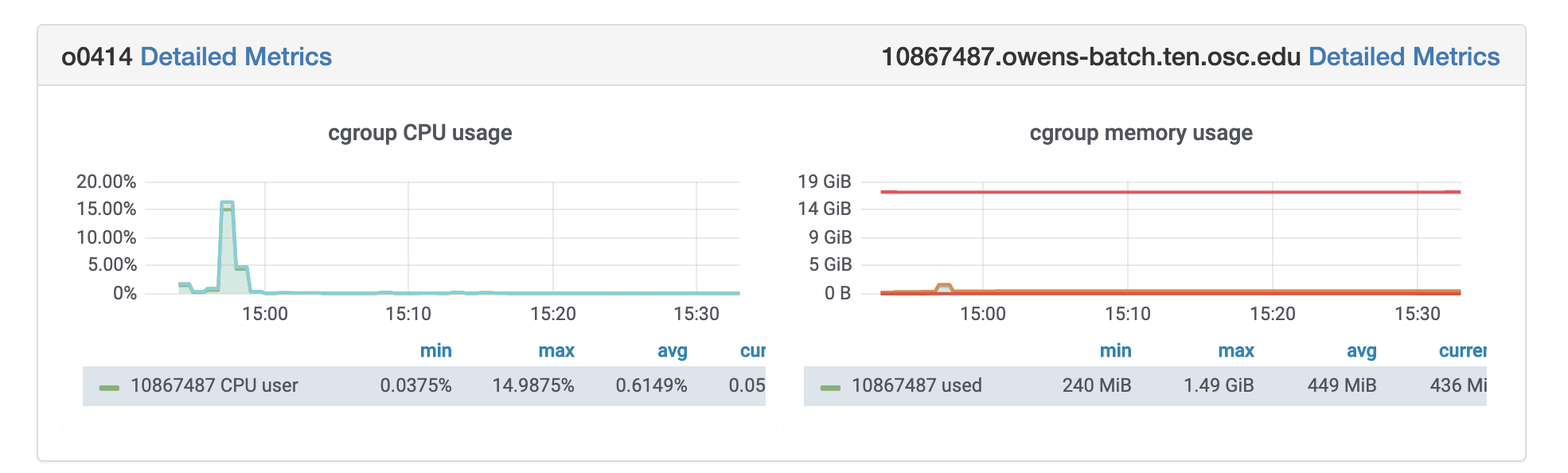
OSC jobs can be monitored for CPU and memory usage using grafana. If your job is in running status, you can get grafana metrics as follows. After log in to OSC OnDemand, select Jobs from the top tabs, then select Active Jobs and then Job that you are interested to profile. You will see grafana metrics at the bottom of the page and you can click on detailed metrics to access more information about your job at grafana.

Screen Shot 2020-07-29 at 3.33.14 PM.png

Rprof:

R’s built-in tool,Rprof function can be used to profile R expressions and the summaryRprof function to summarize the result. More information can be found here.

Here is an example of profiling R code with Rprofe for data analysis on Faithful data.

Rprof("Rprof-out.prof",memory.profiling=TRUE, line.profiling=TRUE)
  data(faithful)
  summary(faithful)
  plot(faithful)
Rprof(NULL)

To analyze profiled data, runsummaryRprof on Rprof-out.prof

summaryRprof("Rprof-out.prof")

You can read more about summaryRprofhere.

Profvis:

It provides an interactive graphical interface for visualizing data from Rprof.

library(profvis)
profvis({
    data(faithful)
    summary(faithful)
    plot(faithful)
},prof_output="profvis-out.prof")

If you are running the R code on Rstudio, it will automatically open up the visualization for the profiled data. More info can be found here.

Using Rstudio for classroom

OSC provides an isolated and custom R environment for each classroom project that requires Rstudio. More information can be found here.

RNA-SeQC

RNA-SeQC is a java program which computes a series of quality control metrics for RNA-seq data. The input can be one or more BAM files. The output consists of HTML reports and tab delimited files of metrics data. This program can be valuable for comparing sequencing quality across different samples or experiments to evaluate different experimental parameters. It can also be run on individual samples as a means of quality control before continuing with downstream analysis.

Availability and Restrictions

Versions

The following versions of RNA-SeQC are available on OSC clusters:

Version	Owens
1.1.8	X*

* Current default version

You can use module spider rna-seqc to view available modules for a given machine. Feel free to contact OSC Help if you need other versions for your work.

Access

RNA-SeQC is available to all OSC users. If you have any questions, please contact OSC Help.

Publisher/Vendor/Repository and License Type

The Broad Insitute, Open source

Usage

Usage on Owens

Set-up

To configure your environment for use of RNA-SeQC, run the following command: module load rna-seqc. The default version will be loaded. To select a particular RNA-SeQC version, use module load rna-seqc/version. For example, use module load rna-seqc/1.1.8 to load RNA-SeQC 1.1.8.

Usage

This software is a Java executable .jar file; thus, it is not possible to add to the PATH environment variable.

From module load rna-seqc, a new environment variable, RNA_SEQC, will be set. Thus, users can use the software by running the following command: java -jar $RNA_SEQC {other options}.

Relion

Relion (REgularised LIkelihood OptimisatioN) is a stand-alone computer program for the refinement of 3D reconstructions or 2D class averages in electron cryo-microscopy.

Availability and Restrictions

Versions

Relion is available on the Owens cluster. The versions currently available at OSC are:

Version	Owens	Pitzer
2.0	X*
3.0.4	X	X
3.1	X*	X*
3.1-gpu	X	X

* Current Default Version

You can use module spider relion2 for version 2.0 or module spider relion for version 3 to view available modules for a given machine. Feel free to contact OSC Help if you need other versions for your work.

Access

Relion is available to all OSC users.

Publisher/Vendor/Repository and License Type

MRC Lab of Molecular Biology, Open source

Usage

Usage on Owens

Set-up

To set up the environment for Relion on the Owens cluster, use the command:

module load relion2/version

module load relion/version

where version is chosen from the available versions (omitting the version will load the default version).

Usage on Pitzer

Set-up

To set up the environment for Relion on the Pitzer cluster, use the command:

module load relion/version

where version is chosen from the available versions (omitting the version will load the default version).

Rosetta

Rosetta is a software suite that includes algorithms for computational modeling and analysis of protein structures. It has enabled notable scientific advances in computational biology, including de novo protein design, enzyme design, ligand docking, and structure prediction of biological macromolecules and macromolecular complexes.

Availability and Restrictions

Versions

The Rosetta suite is available on Owens and Pitzer. The versions currently available at OSC are:

Version	Owens	Pitzer
3.10	X	X
3.12	X*	X*

* Current default version

You can use module spider rosetta to view available modules for a given machine. Feel free to contact OSC Help if you need other versions for your work.

Access for Academic Users

Rosetta is available to academic OSC users. Please review the license agreement carefully before use. If you have any questions, please contact OSC Help.

Publisher/Vendor/Repository and License Type

Rosetta, Non-Commercial

Usage

Usage on Owens and Pitzer

To set up your environment for rosetta load one of its module files:

module load rosetta/3.10

Here is an example batch script that uses Rosetta Abinitio Relax application via the batch system:

# Example Rosetta Abinitio Relax application batch script.
#PBS -N rosetta_abinitio_relax
#PBS -j oe
#PBS -m ae
#PBS -l walltime=0:20:00
#PBS -l nodes=1:ppn=1
#PBS -S /bin/sh

qstat -f $PBS_JOBID
export

module load intel
module load rosetta
module list

cd $PBS_O_WORKDIR
pbsdcp -rp $OSC_ROSETTA_HOME/demos/tutorials/denovo_structure_prediction/* $TMPDIR
cd $TMPDIR
AbinitioRelax.linuxiccrelease @input_files/options

ls -l
pbsdcp -rp '*' $PBS_O_WORKDIR

SAMtools

SAM format is a generic format for storing large nucleotide sequence alignments. SAMtools provide various utilities for manipulating alignments in the SAM format, including sorting, merging, indexing and generating alignments in a per-position format.

Availability and Restrictions

The following versions of SAMtools are available on OSC clusters:

Version	Owens	Pitzer
1.3.1	X
1.6	X
1.8		X
1.9	X
1.10	X*	X*

* Current default version

You can use module spider samtools to view available modules for a given machine. Feel free to contact OSC Help if you need other versions for your work.

Access

SAMtools is available to all OSC users. If you have any questions, please contact OSC Help.

Publisher/Vendor/Repository and License Type

Genome Research Ltd., Open source

Usage

Usage on Owens

Set-up

To configure your environment for use of SAMtools, run the following command: module load samtools . The default version will be loaded. To select a particular SAMtools version, use module load samtools/version . For example, use module load samtools/1.3.1 to load SAMtools 1.3.1.

Usage on Pitzer

Set-up

To configure your environment for use of SAMtools, run the following command: module load samtools . The default version will be loaded.

SIESTA

SIESTA is both a method and its computer program implementation, to perform efficient electronic structure calculations and ab initio molecular dynamics simulations of molecules and solids. More information can be found from here.

Availability and Restrictions

Versions

SIESTA is available on the Owens and Oakley clusters. A serial and a parallel build were created in order to meet users' computational needs.

Version	Owens	Pitzer
4.0	X
4.0.2	X*	X*

* Current default version

You can use module spider siesta to view available modules for a given machine. Feel free to contact OSC Help if you need other versions for your work.

Access

SIESTA newer than version 4.0 is under GPL license. Therefore, any users can access SIESTA on Owens. If you have any questions, please contact OSC Help for further information.

Publisher/Vendor/Repository and License Type

https://departments.icmab.es/leem/siesta/, Open source

Usage

Batch Usage

When you log into oakley.osc.edu or owens.osc.edu, you are actually logged into a linux box referred to as the login node. To gain access to the 4000+ processors in the computing environment, you must submit your SIESTA job to the batch system for execution.

Assume that you have a test case in your work directory (where you submit your job, represented by $PBS_O_WORKDIR), with the input file 32_h2o.fdf. A batch script can be created and submitted for a serial or parallel run. The following are the sample batch scripts for running serial and parallel SIESTA jobs. Sample batch scripts and input files are also available here:

~srb/workshops/compchem/siesta/

Sample Batch Script for Serial Jobs

#!/bin/bash
#SBATCH --time=0:30:00
#SBATCH --nodes=1 --ntasks-per-node=28
#SBATCH --job-name=siesta
#SBATCH --account <project-account>
#
# Set up the package environment
module load siesta
#
# Execute the serial solver (nodes=1, ppn<=12)
siesta <32_h2o.fdf> output
exit

NOTE: Change ntasks-per-node to = 28 for Owens

Sample Batch Script for Parallel Jobs

#!/bin/bash
#SBATCH --time=0:30:00
#SBATCH --nodes=2 --ntasks-per-node=28
#SBATCH --job-name=siesta
#SBATCH --account <project-account> 
#
# Set up the package environment
module swap intel/12.1.4.319 intel/13.1.3.192
module load siesta_par
#
# Execute the parallel solver (nodes>1, ppn=28)
srun siesta <32_h2o.fdf> output
exit

NOTE: Change ntasks-per-node to = 28 for Owens

Usage on Pitzer

#!/bin/bash
#SBATCH --time=0:30:00 
#SBATCH --nodes=1 --ntasks-per-node=48
#SBATCH --job-name=siesta
#SBATCH --account <project-account> 
#
# Set up the package environment
module load siesta
#
# Execute the serial solver (nodes=1, ppn<=48)
siesta <32_h2o.fdf> output
exit

Citations

This is required for the versions older than 4.0.

1. “Self-consistent order-N density-functional calculations for very large systems”, P. Ordejón, E. Artacho and J. M. Soler, Phys. Rev. B (Rapid Comm.) 53, R10441-10443 (1996).

2. “The SIESTA method for ab initio order-N materials simulation”, J. M. Soler, E. Artacho,J. D. Gale, A. García, J. Junquera, P. Ordejón, and D. Sánchez-Portal, J. Phys.: Condens. Matt. 14, 2745-2779 (2002).

Supercomputer:

Service:

Fields of Science:

SRA Toolkit

The Sequence Read Archive (SRA Toolkit) stores raw sequence data from "next-generation" sequencing technologies including 454, IonTorrent, Illumina, SOLiD, Helicos and Complete Genomics. In addition to raw sequence data, SRA now stores alignment information in the form of read placements on a reference sequence. Use SRA Toolkit tools to directly operate on SRA runs.

NCBI blocks any connection from computing nodes because they are behind firewalls. Thus OSC users cannot use SRA tools to download data "on-the-fly" at runtime or fetch data on computing nodes, e.g. 'fastq-dump -X 5 SRR390728' or 'prefetch SRR390728'. OSC users must download SRA data on login nodes using the command 'prefetch' before any sequence analysis. Please read the section Download SRA Data below to learn how to download and use SRA data.

Availability and Restrictions

The following versions of SRA Toolkit are available on OSC clusters:

Version	Owens	Pitzer
2.6.3	X
2.9.0	X
2.9.1		X
2.9.6	X*	X*
2.10.7	X	X

* Current default version

You can use module spider sratoolkit to view available modules for a given machine. Feel free to contact OSC Help if you need other versions for your work.

Access

SRA Toolkit is available to all OSC users. If you have any questions, please contact OSC Help.

Publisher/Vendor/Repository and License Type

National Center for Biotechnology Information, Freeware

Usage

Usage on Pitzer and Owens

Set-up

To configure your environment for use of SRA Toolkit, run the following command: module load sratoolkit. The default version will be loaded. To select a particular SRA Toolkit version, use module load sratoolkit/version. For example, use module load sratoolkit/2.9.6 to load SRA Toolkit 2.9.6

Download SRA Data

NCBI has shifted to using cloud-style object stores. Aspera support requires Cloud credential :https://github.com/ncbi/sra-tools/wiki/04.-Cloud-Credentials.

The issue has been reported here.

You can download SRA data to local directory with prefetch

$ module load sratoolkit/2.9.6
$ prefetch SRR390728

If it is your first time to use Toolkit, you might encounter some errors. Please refer here for Toolkit configuration.

The default download path is in your home directory ~/ncbi/public. For example, you can find the SRA file SRR390728.sra in ~/ncbi/public/sra and the resource files in ~/ncbi/public/refseq. Use srapath to check if the SRA accession is available in the download path

$ srapath SRR390728
/users/PAS1234/johndoe/ncbi/public/sra/SRR390728.sra

Now you can run other SRA tools, e.g. fastq-dump on computing nodes. Here is a job script example:

#!/bin/bash
#SBATCH --job-name use_fastq_dump
#SBATCH --time=0:10:0
#SBATCH --nodes=1 --ntasks-per-node=1

module load sratoolkit/2.9.6
module list
fastq-dump -X 5 -Z ~/ncbi/public/sra/SRR390728.sra

However, our Home Directory file system is not suitable for heavy computation. If the SRA file is large, you can consider the following options for better performance.

Change default download path to a faster file system, i.e. /fs/scratch

You can change the default download path for SRA data to our scratch file system with one of following two approaches. For example, /fs/scratch/PAS1234/johndoe/ncbi:

#
### Approach 1.
#
$ mkdir -p /fs/scratch/PAS1234/johndoe/ncbi # create ncbi directory in scratch if you don't have one
$ module load sratoolkit/2.9.x
$ vdb-config --set /repository/user/main/public/root=/fs/scratch/PAS1234/johndoe/ncbi
$ prefetch SRR390728
$ srapath SRR390728
/fs/scratch/PAS1234/johndoe/ncbi/sra/SRR390728.sra

#
### Approach 2. CAUTION: make sure no working data in ~/ncbi
# 
$ rm -rf ~/ncbi/*
$ rmdir ~/ncbi
$ mkdir -p /fs/scratch/PAS1234/johndoe/ncbi # create ncbi directory in scratch if you don't have one
$ ln -s  /fs/scratch/PAS1234/johndoe/ncbi ~/ncbi
$ module load sratoolkit/2.9.x
$ prefetch SRR390728
$ srapath SRR390728
/users/PAS1234/johndoe/ncbi/sra/SRR390728.sra

#
### Approach 3. sratoolkit/2.10.x only
# 
$ module load sratoolkit/2.10.x 
$ vdb-config --prefetch-to-cwd
$ mkdir -p /fs/scratch/PAS1234/johndoe/ncbi # create ncbi directory in scratch if you don't have one 
$ cd /fs/scratch/PAS1234/johndoe/ncbi
$ prefetch SRR390728
$ srapath SRR390728
/fs/scratch/PAS1234/johndoe/ncbi/SRR390728

Your SRA data would be stored in /fs/scratch/PAS1234/johndoe/ncbi

STAR

STAR: Spliced Transcripts Alignment to a Reference.

Availability and Restrictions

Versions

The following versions of STAR are available on OSC clusters:

Version	Owens
2.5.2a	X*
2.6.0a	X

* Current default version

You can use module spider star to view available modules for a given machine. Feel free to contact OSC Help if you need other versions for your work.

Access

STAR is available to all OSC users. If you have any questions, please contact OSC Help.

Publisher/Vendor/Repository and License Type

Alexander Dobin, Open source

Usage

Usage on Owens

Set-up

To configure your environment for use of STAR, run the following command: module load star. The default version will be loaded. To select a particular STAR version, use module load star/version. For example, use module load star/2.5.2a to load STAR 2.5.2a.

STAR-CCM+

STAR-CCM+ provides the world’s most comprehensive engineering physics simulation inside a single integrated package. Much more than a CFD code, STAR‑CCM+ provides an engineering process for solving problems involving flow (of fluids and solids), heat transfer and stress. STAR‑CCM+ is unrivalled in its ability to tackle problems involving multi‑physics and complex geometries. Support is provided by CD-adapco. CD-adapco usually releases new version of STAR-CCM+ every four months.

Availability and Restrictions

Versions

STAR-CCM+ is available on the Owens Cluster. The versions currently available at OSC are:

Version	Owens
11.02.010	X
11.06.011	X
12.04.010	X
12.06.010	X
13.02.011	X
13.04.011	X
14.02.010	X
14.04.013	X
15.02.007	X*
15.06.008	X

* Current default version

We have STAR-CCM+ Academic Pack, which includes STAR-CCM+, STAR-innovate, CAD Exchange, STAR-NX, STAR-CAT5, STAR-Inventor, STAR-ProE, JTOpen Reader, EHP, Admixturs, Vsim, CAT, STAR-ICE, Battery Design Studio, Sattery Simulation Module, SPEED, SPEED/Enabling PC-FEA, SPEED/Optimate, DARS, STAR-CD, STAR-CD/Reactive Flow Models, STAR-CD/Motion, esiece, and pro-STAR.

You can use module spider starccm to view available modules for a given machine. The default versions are in double precision. Please check with module spider starccm to see if there is a mixed precision version available. Feel free to contact OSC Help if you need other versions for your work.

Access for Academic Users

Academic users can use STAR-CCM+ on OSC machines if the user or user's institution has proper STAR-CCM+ license. Currently, users from Ohio State University, University of Cincinnati, University of Akron, and University of Toledo can access the OSC's license.

Use of STAR-CCM+ for academic purposes requires validation. In order to obtain validation, please contact OSC Help for further instruction.

Currently, OSC has a 50 seat license (ccmpsuite, which allows up to 50 concurrent users), with 10,000 additional core licenses (hpcdomains) for academic users.

Access for Commerical Users

Contact OSC Help for getting access to STAR-CCM+ if you are a commerical user.

Publisher/Vendor/Repository and License Type

Siemens, Commercial

Usage

Usage on Owens

Set-up on Owens

We recommend to run STAR-CCM+ on only the compute nodes. Thus, all STAR-CCM+ jobs should be submitted via the batch scheduling system, either as interactive or non-interactive batch jobs. To load the default version of STAR-CCM+ module on Owens, use module load starccm . To select a particular software version, use module load starccm/version . For example, use module load starccm/11.02.010 to load STAR-CCM+ version 11.02.010 on Owens.

Batch Usage on Owens

When you log into owens.osc.edu you are actually logged into a linux box referred to as the login node. To gain access to the mutiple processors in the computing environment, you must submit your STAR-CCM+ analysis to the batch system for execution. Batch jobs can request mutiple nodes/cores and compute time up to the limits of the OSC systems. Refer to Queues and Reservations and Batch Limit Rules for more info. Batch jobs run on the compute nodes of the system and not on the login node. It is desirable for big problems since more resources can be used. STAR-CCM+ can be run on OSC clusters in either interactive mode or in non-interactive batch mode.

Interactive Batch Session

Interactive mode is similar to running STAR-CCM+ on a desktop machine in that the graphical user interface (GUI) will be sent from OSC and displayed on the local machine. To run interactive STAR-CCM+, it is suggested to request necessary compute resources from the login node, with X11 forwarding. The intention is that users can run STAR-CCM+ interactively for the purpose of building their model, preparing input file (.sim file), and checking results. Once developed this input file can then be run in no-interactive batch mode. For example, the following line requests one node with 28 cores( -N 1 -n 28 ), for a walltime of one hour ( -t 1:00:00 ), with one STAR-CCM+ base license token ( -L starccm@osc:1 ) on Owens:

sinteractive -N 1 -n 28 -t 1:00:00 -L starccm@osc:1

This job will queue until resources become available. Once the job is started, you're automatically logged in on the compute node; and you can launch STAR-CCM+ GUI with the following commands:

module load starccm
starccm+ -mesa

Non-interactive Batch Job (Serial Run using 1 Base Token)

A batch script can be created and submitted for a serial or parallel run. You can create the batch script using any text editor you like in a working directory on the system of your choice.

Below is the example batch script ( job.txt ) for a serial run with an input file ( starccm.sim ) on Owens:

#!/bin/bash
#SBATCH --job-name=starccm_test
#SBATCH --time=1:00:00
#SBATCH --nodes=1 --ntasks-per-node=1
#SBATCH -L starccm@osc:1

cd $TMPDIR  
cp $SLURM_SUBMIT_DIR/starccm.sim .  
module load starccm  
starccm+ -batch starccm.sim >&output.txt  
cp output.txt $SLURM_SUBMIT_DIR

To run this job on OSC batch system, the above script is to be submitted with the command:

sbatch job.txt

Non-interactive Batch Job (Parallel Run using HPC Tokens)

To take advantage of the powerful compute resources at OSC, you may choose to run distributed STAR-CCM+ for large problems. Multiple nodes and cores can be requested to accelerate the solution time. The following shows an example script if you need 2 nodes with 28 cores per node on Owens using the inputfile named starccm.sim :

#!/bin/bash
#SBATCH --job-name=starccm_test
#SBATCH --time=3:00:00
#SBATCH --nodes=2 --ntasks-per-node=28
#SBATCH -L starccm@osc:1,starccmpar@osc:56

cp starccm.sim $TMPDIR
cd $TMPDIR
module load 

srun hostname | sort -n > ${SLURM_JOB_ID}.nodelist

starccm+ -np 56 -batch -machinefile ${SLURM_JOB_ID}.nodelist -mpi intel -mpiflags '-rmk slurm' -rsh ssh starccm.sim >&output.txt
cp output.txt $SLURM_SUBMIT_DIR

In addition to requesting the STAR-CCM+ base license token ( -L starccm@osc:1 ), you need to request copies of the starccmpar license, i.e., HPC tokens ( -L starccm@osc:1,starccmpar@osc:[n] ), where [n] is equal to the number of cores.

Run STAR-CCM+ to STAR-CCM+ Coupling

This documentation is to discuss how to run STAR-CCM+ to STAR-CCM+ Coupling simulation in batch job at OSC. The following example demonstrates the process of using STAR-CCM+ version 11.02.010 on Owens. Depending on the version of STAR-CCM+ and cluster you work on, there mighe be some differences from the example. Feel free to contact OSC Help if you have any questions.

Prepare Lagging Simulation

Launch the STAR-CCM+ GUI following the instructions on this page
Load the simulation that lags and prepare the lagging simulation following the STAR-CCM+ User Guide
- Active a co-simulation model
- Set "Concurrency mode -> Method" to Lag
- Other setups
Save the lagging simulation and name it for example as lag.sim

Prepare Leading Simulation

Load the simulation that leads and prepare the leading simulation following the STAR-CCM+ User Guide
- Active a co-simulation model
- Set "Concurrency mode -> Method" to Lead
Go to the "Connect Method" node by selecting "Co-Simulations -> <name of co-simulation> -> Conditions". Click "Edit" of "Connect Method". In "Connect Method" node, select "Launch Application and Connect" under method. Under "Launch Application and Connect", put the following information as "Launch Command":

/usr/local/starccm/11.02.010/STAR-CCM+11.02.010-R8/star/bin/starccm+ -load -server -rsh /usr/local/bin/pbsrsh lag.sim

See the picture below:

connect method

Save the leading simulation and name it for example as lead.sim

Prepare Job Script

In the job script, use the following command to run the co-simulation:

starccm+ -np N,M -rsh /usr/local/bin/pbsrsh -batch -machinefile $PBS_NODEFILE lead.sim

where N is # of cores for the leading simulation and M is # of cores for the lagging simulation, and the summation of N and M should be the total number of cores you request in the job.

Once the job is completed, the output results of the leading simulation will be returned, while the lagging simulation runs on the background server and the final results won't be saved.

Supercomputer:

Service:

Fields of Science:

https://www.osc.edu/resources/getting_started/howto/howto_install_tensorflow_locally

STAR-Fusion

STAR-Fusion is a component of the Trinity Cancer Transcriptome Analysis Toolkit (CTAT). STAR-Fusion uses the STAR aligner to identify candidate fusion transcripts supported by Illumina reads. STAR-Fusion further processes the output generated by the STAR aligner to map junction reads and spanning reads to a reference annotation set.

Availability and Restrictions

Versions

The following versions of STAR-Fusion are available on OSC clusters:

Version	Owens
0.7.0	X*
1.4.0	X

* Current default version

You can use module spider star-fusion to view available modules for a given machine. Feel free to contact OSC Help if you need other versions for your work.

Access

STAR-Fusion is available to all OSC users. If you have any questions, please contact OSC Help.

Publisher/Vendor/Repository and License Type

Broad Institute, Open source

Usage

Usage on Owens

Set-up

To configure your environment for use of STAR-Fusion, run the following command: module load star-fusion. The default version will be loaded. To select a particular STAR-Fusion version, use module load star-fusion/version. For example, use module load star-fusion/0.7.0 to load STAR-Fusion 0.7.0.

Salmon

Salmon is a tool for quantifying the expression of transcripts using RNA-seq data.

Availability and Restrictions

Versions

Salmon is available on the Owens Cluster. The versions currently available at OSC are:

Version	Owens
0.8.2	X*
1.0.0	X

* Current default version

You can use module spider salmonto view available modules for a given machine. Feel free to contact OSC Help if you need other versions for your work.

Access

Salmon is available to all OSC users. If you have any questions, please contact OSC Help.

Publisher/Vendor/Repository and License Type

Patro, R. et al., Freeware

Usage

Usage on Owens

Set-up

To configure your enviorment for use of Salmon, use command module load salmon. This will load the default version.

ScaLAPACK

ScaLAPACK is a library of high-performance linear algebra routines for clusters supporting MPI. It contains routines for solving systems of linear equations, least squares problems, and eigenvalue problems.

This page documents usage of the ScaLAPACK library installed by OSC from source. An optimized implementation of ScaLAPACK is included in MKL; see the software documentation page for Intel Math Kernel Library for usage information.

Availability and Restrictions

Versions

The versions currently available at OSC are:

Version	Owens	Pitzer
2.0.2	X	X
2.1.0	X*	X*

* Current default version

You can use module spider scalapack to view available modules for a given machine. Feel free to contact OSC Help if you need other versions for your work.

Access

ScaLAPACK is available to all OSC users. If you need high performance, we recommend using MKL instead of the standalone ScaLAPACK module. If you have any questions, please contact OSC Help.

Publisher/Vendor/Repository and License Type

Univ. of Tennessee; Univ. of California, Berkeley; Univ. of Colorado Denver; and NAG Ltd./ Open source

Usage

Usage on Owens

Set-up

Initalizing the system for use of the ScaLAPACK libraries is dependent on the system you are using and the compiler you are using. To use the ScaLAPACK libraries in your compilation, run the following command: module load scalapack. To load a particular version, use module load scalapack/version. For example, use module load scalapack/2.0.2 to load ScaLAPACK version 2.0.2. You can use module spider scalapack to view available modules.

Building with ScaLAPACK

Once loaded, the ScaLAPACK libraries can be linked in with your compilation. To do this, use the following environment variables. You must also link with MKL. With the Intel compiler, just add -mkl to the end of the link line. With other compilers, load the mkl module and add $MKL_LIBS to the end of the link line.

Variable	Use
`$SCALAPACK_LIBS`	Used to link ScaLAPACK into either Fortran or C

Usage on Pitzer

Set-up

Building with ScaLAPACK

VARIABLE	USE
`$SCALAPACK_LIBS`	Used to link ScaLAPACK into either Fortran or C

Schrodinger

The Schrodinger molecular modeling software suite includes a number of popular programs focused on drug design and materials science but of general applicability, for example Glide, Jaguar, and MacroModel. Maestro is the graphical user interface for the suite. It allows the user to construct and graphically manipulate both simple and complex chemical structures, to apply molecular mechanics and dynamics techniques to evaluate the energies and geometries of molecules in vacuo or in solution, and to display and examine graphically the results of the modeling calculations.

Availability and Restrictions

Versions

The Schrodinger suite is available on Owens. The versions currently available at OSC are:

Version	Owens
15	X
16	X
2018.3	X
2019.3	X
2020.1	X*

* Current default version

You can use module spider schrodinger to view available modules for a given machine. Feel free to contact OSC Help if you need other versions for your work.

Access

Schrodinger is available to all academic users.

To use Schrodinger you will have to be added to the license server first. Please contact OSC Help to be added. Please note that if you are a non-OSU user, we need to send your name, contact email, and affiliation information to Schrodinger in order to grant access. Currently, we have license for following features:

CANVAS_ELEMENTS
CANVAS_MAIN
CANVAS_SHARED
COMBIGLIDE_MAIN
EPIK_MAIN
FFLD_OPLS_MAIN
GLIDE_MAIN
GLIDE_XP_DESC
IMPACT_MAIN
KNIME_MAIN
LIGPREP_MAIN
MAESTRO_MAIN
MMLIBS
MMOD_CONFGEN
MMOD_MACROMODEL
MMOD_MBAE
QIKPROP_MAIN

You need to use one of following software flags in order to use the particular feature of the software without license errors.

macromodel, glide, ligprep, qikprep, epik

You can add -L glide@osc:1 to your job script if you use GLIDE for example. When you use this software flag, then your job won't start until it secures available licenses. Please read the batch script examples down below.

Publisher/Vendor/Repository and License Type

Schrodinger, LLC/ Commercial

Usage

Usage on Owens

To set up your environment for schrodinger load one of its modulefiles:

module load schrodinger/schrodinger16

Using schrodinger interactively requires an X11 connection. Typically one will launch the graphical user interface:

maestro

Here is an example batch script that uses schrodinger non-interactively via the batch system:

#!/bin/bash
# Example glide single node batch script.
#SBATCH --job-name=glidebatch
#SBATCH --time=1:00:00
#SBATCH --nodes=1 --ntasks-per-node=28
#SBATCH -L glide@osc:1

module load schrodinger
cp * $TMPDIR
cd $TMPDIR
host=`srun hostname|head -1`
nproc=`srun hostname|wc -l`
glide -WAIT -HOST ${host}:${nproc} receptor_glide.in
ls -l
cp * $SLURM_SUBMIT_DIR

The glide command passes control to the Schrodinger Job Control utility which processes the two options: The WAIT option forces the glide command to wait until all tasks of the command are completed. This is necessary for the batch jobs to run effectively. The HOST option specifies how tasks are distributed over processors.

Singularity

Singularity is a container system designed for use on High Performance Computing (HPC) systems. It allows users to run both Docker and Singularity containers.

From the Docker website: "A container image is a lightweight, stand-alone, executable package of a piece of software that includes everything needed to run it: code, runtime, system tools, system libraries, settings."

Availability and Restrictions

Versions

Singularity is available on Ruby, Owens and Pitzer clusters. Only one version is available at any given time. To find out the current version:

singularity version

Check the release page for the changelog: https://github.com/sylabs/singularity/releases

Access

Singularity is available to all OSC users.

Publisher/Vendor/Repository and License Type

SyLabs, Inc., 3-clause BSD License

Usage

Set-up

No setup is required. You can use Singulairty directly on all clusters.

Using Singularity

See HOWTO: Use Docker and Singularity Containers at OSC for information about using Singularity on Ruby, Owens and Pitzer clusters, including some site-specific caveats.

Example: Run a container from the Singularity hub

[owens-login01]$ singularity run shub://singularityhub/hello-world
INFO:    Downloading library image
Tacotacotaco

Known Issues

Failed to pull a large Docker image

Update: 05/21/2019
Version: all

You might encounter an error while pulling a large Docker image:

[owens-login01]$ singularity pull docker://qimme2/core
FATAL: Unable to pull docker://qiime2/core While running mksquashfs: signal: killed

The process could be killed because the image is cached in the home directory which is a slower file system or the image size might exceed a single file size limit.

The solution is to use other file systems like /fs/scratch and $TMPDIR for caches and temp files to build the squashfs filesystem:

[owens-login01]$ sinteractive -n 1 -A PAS1234 
bash-4.2$ export SINGULARITY_CACHEDIR=$TMPDIR
bash-4.2$ export SINGULARITY_TMPDIR=$TMPDIR 
bash-4.2$ singularity pull docker://qiime2/core:2019.1
INFO:    Converting OCI blobs to SIF format
INFO:    Starting build...
...
INFO:    Creating SIF file...
bash-4.2$ exit

Failed to run a container directly or pull an image from Singularity or Docker hub

Update: 03/08/2019
Version: all

You might encounter an error while run a container directly from a hub:

[owens-login01]$ singularity run shub://vsoch/hello-world
Progress |===================================| 100.0%
FATAL: container creation failed: mount error: can't mount image /proc/self/fd/13: failed to find loop device: could not attach image file too loop device: No loop devices available

One solution is to remove the Singularity cached images from local cache directory $HOME/.singularity/cache. If the singularity version is prior to 3.0:

[owens-login01]$ cd $HOME/.singularity/cache
[owens-login01 cache]$ rm -rf *

If the singularity version is 3.1 and above:

[owens-login01]$ singulariy cache clean

Alternatively, you can change the Singularity cache directory to different location by setting the variable SINGULARITY_CACHEDIR. For example, in a batch job:

#/bin/bash
#SBATCH --job-name="singularity_test"
#SBSTCH --ntasks=1

export SINGULARITY_CACHEDIR=$TMPDIR
singularity run shub://vsoch/hello-world

Workshop

2019-05-14 OSC Workshop: Containers for Research Computing. Please find the link in the workshop page for the tutorial material and slides.

SnpEff

SnpEff is a variant annotation and effect prediction tool. It annotates and predicts the effects of variants on genes (such as amino acid changes).

Availability and Restrictions

Versions

The following versions of SnpEff are available on OSC clusters:

Version	Owens
4.2	X*

* Current default version

You can use module spider snpeff to view available modules for a given machine. Feel free to contact OSC Help if you need other versions for your work.

Access

SnpEff is available to all OSC users. If you have any questions, please contact OSC Help.

Publisher/Vendor/Repository and License Type

http://snpeff.sourceforge.net, Open source

Usage

Usage on Owens

Set-up

To configure your environment for use of SnpEff, run the following command: module load snpeff. The default version will be loaded. To select a particular SnpEff version, use module load snpeff/version. For example, use module load snpeff/4.2 to load SnpEff 4.2.

Usage

This software consists of Java executable .jar files; thus, it is not possible to add to the PATH environment variable.

From module load snpeff, new environment variables, SNPEFF and SNPSIFT, will be set. Thus, users can use the software by running the following command: java -jar $SNPEFF {other options}, or java -jar $SNPSIFT {other options}.

Spark

Apache Spark is an open source cluster-computing framework originally developed in the AMPLab at University of California, Berkeley but was later donated to the Apache Software Foundation where it remains today. In contrast to Hadoop's disk-based analytics paradigm, Spark has multi-stage in-memory analytics. Spark can run programs up-to 100x faster than Hadoop’s MapReduce in memory or 10x faster on disk. Spark support applications written in python, java, scala and R

Availability and Restrictions

Versions

The following versions of Spark are available on OSC systems:

Version	Owens	Pitzer	Note
2.0.0	X*		Only support Python 3.5
2.1.0	X		Only support Python 3.5
2.3.0	X
2.4.0	X	X*
2.4.5	X	X

* Current default version

You can use module spider spark to view available modules for a given machine. Feel free to contact OSC Help if you need other versions for your work.

Access

Spark is available to all OSC users. If you have any questions, please contact OSC Help.

Publisher/Vendor/Repository and License Type

The Apache Software Foundation, Open source

Usage

Set-up

In order to configure your environment for the usage of Spark, run the following command:

module load spark

A particular version of Spark can be loaded as follows

module load spark/2.3.0

Using Spark

In order to run Spark in batch, reference the example batch script below. This script requests 6 node on the Owens cluster for 1 hour of walltime. The script will submit the pyspark script called test.py using pbs-spark-submit command.

#!/bin/bash 
#SBATCH --job-name ExampleJob 
#SBATCH --nodes=2 --ntasks-per-node=48 
#SBATCH --time=01:00:00 
#SBTACH --account your_project_id

module load spark

cp test.py $TMPDIR
cd $TMPDIR 

pbs-spark-submit test.py  > test.log

cp * $SLURM_SUBMIT_DIR

pbs-spark-submit script is used for submitting Spark jobs. For more options, please run,

pbs-spark-submit --help

Running Spark interactively in batch

To run Spark interactively, but in batch on Owens please run the following command,

 sinteractive -N 2 -n 28 -t 01:00:00

When your interactive shell is ready, please launch spark cluster using the pbs-spark-submit script

pbs-spark-submit

You can then launch pyspark by connecting to Spark master node as follows.

pyspark --master spark://nodename.ten.osc.edu:7070

Launching Jupyter+Spark on OSC OnDemand

Instructions on how to launch Spark on OSC OnDemand web interface is here. https://www.osc.edu/content/launching_jupyter_spark_app

Example Jobs

Please check /usr/local/src/spark/2.0.0/test.osc folder for more examples of pyspark script, job submission script and output files.

Stata

Stata is a complete, integrated statistical package that provides everything needed for data analysis, data management, and graphics. 32-processor MP version is currently available at OSC.

Availability and Restrictions

Versions

The following versions of Stata are available on OSC systems:

Version	Owens
15	X*

* Current default version

You can use module spider stata to view available modules for a given machine. Feel free to contact OSC Help if you need other versions for your work.

Access

Only academic OSC users can use the software. OSC has the license for 5 seats concurrently. Each user can use up to 32 cores. In order to access the software, please contact OSC Help to get validated.

Publisher/Vendor/Repository and License Type

StataCorp, LLC, Commercial

Usage

Set-up

To configure your environment on Oakley for the usage of Stata, run the following command:

module load stata

Using Stata

Due to licensing restrictions, Stata may ONLY be used via the batch system on Owens. See below for information on how this is done.

Batch Usage

OSC has a 5-user license. However, there is no enforcement mechanism built into Stata. In order for us to stay within the 5-user limit, we require you to run in the context of SLURM and to include this option when starting your batch job (the SLURM system will enforce the 5 user limit):

#SBATCH -L stata@osc:1

Non-Interactive batch example

Use the script below as a template for your usage.

#!/bin/bash
#SBATCH -t 1:00:00
#SBATCH --nodes=1 --ntask-per-node=28
#SBATCH -L stata@osc:1
#SBATCH --job-name=stata

module load stata

stata-mp -b do bigjob

StringTie

StringTie assembles aligned RNA-Seq reads into transcripts that represent splice variants in RNA-Seq samples.

Availability and Restrictions

Versions

StringTie is available on the Owens Cluster. The versions currently available at OSC are:

Version	Owens
1.3.3b	X*

* Current Default Version

You can use module spider stringtieto view available modules for a given machine. Feel free to contact OSC Help if you need other versions for your work.

Access

StringTie is available to all OSC users. If you have any questions, please contact OSC Help.

Publisher/Vendor/Repository and License Type

https://ccb.jhu.edu/software/stringtie/, Open source

Usage

Usage on Owens

Set-up

To configure your enviorment for use of StringTie, use command module load stringtie. This will load the default version.

Subread

The Subread package comprises a suite of software programs for processing next-gen sequencing read data like Subread, Subjunc, featureCounts, and exactSNP.

Availability and Restrictions

Versions

The following versions of Subread are available on OSC clusters:

Version	Owens
1.5.0-p2	X*

* Current default version

You can use module spider subread to view available modules for a given machine. Feel free to contact OSC Help if you need other versions for your work.

Access

Subread is available to all OSC users. If you have any questions, please contact OSC Help.

Publisher/Vendor/Repository and License Type

http://subread.sourceforge.net, Open source

Usage

Usage on Owens

Set-up

To configure your environment for use of Subread, run the following command: module load subread. The default version will be loaded. To select a particular Subread version, use module load subread/version. For example, use module load subread/1.5.0-p2 to load Subread 1.5.0-p2.

Subversion

Apache Subversion is a full-featured version control system.

Availability and Restrictions

Versions

The following versions of Subversion are available on OSC systems:

Version	Owens
1.8.19	X*

* Current default version

You can use module spider subversion to view available modules for a given machine. Feel free to contact OSC Help if you need other versions for your work.

Access

Subversion is available to all OSC users. If you have any questions, please contact OSC Help.

Publisher/Vendor/Repository and License Type

Apache Software Foundation, Open Source, Apache License

Usage

Set-up

The default version 1.7.14 is system-built. It is ready as you login. To use other versions, e.g 1.8.19 run the following command:

module load subversion/1.8.19

SuiteSparse

SuiteSparse is a suite of sparse matrix algorithms, including: UMFPACK(multifrontal LU factorization), CHOLMOD(supernodal Cholesky, with CUDA acceleration), SPQR(multifrontal QR) and many other packages.

Availability and Restrictions

Versions

OSC supports most packages in SuiteSparse, including UMFPACK, CHOLMOD, SPQR, KLU and BTF, Ordering Methods (AMD, CAMD, COLAMD, and CCOLAMD) and CSparse. SuiteSparse modules are available for the Intel, GNU, and Portland Group compilers. The following versions of SuiteSparse are available at OSC.

Version	Owens
4.5.3	X*

* Current default version

You can use module spider suitesparse to view available modules for a given machine. Feel free to contact OSC Help if you need other versions for your work.

NOTE: SuiteSparse library on our clusters is built without METIS, which might matter if CHOLMOD package is included in your program.

Access

SuiteSparse is available to all OSC users. If you have any questions, please contact OSC Help.

Publisher/Vendor/Repository and License Type

Timothy A. Davis, Patrick R. Amestoy, and Iain S. Duff./ Open source

Usage

Usage on Owens

Set-up on Owens

To use SuitSparse, ensure the correct compiler is loaded. User module spider suitesparse/version to view compatible compilers. Before loading the SuiteSparse library, MKL is also required. Load the MKL library with module load mkl. Then with the following command, SuiteSparse library is ready to be used: module load suitesparse.

Building With SuiteSparse

With the SuiteSparse library loaded, the following environment variables will be available for use:

Variable	Use
$SUITESPARSE_CFLAGS	Include flags for C or C++ programs.
$SUITESPARSE_LIBS	Use when linking your program to SuiteSparse library.

For example, to build the code my_prog.c with the SuiteSparse library you would use:

icc -c my_prog.c
icc -o my_prog my_prog.o $SUITESPARSE_LIBS

Batch Usage on Owens

When you log into oakley.osc.edu you are actually logged into a linux box referred to as the login node. To gain access to the mutiple processors in the computing environment, you must submit your job to the batch system for execution. Batch jobs can request mutiple nodes/cores and compute time up to the limits of the OSC systems. Refer to Queues and Reservations and Batch Limit Rules for more info. Batch jobs run on the compute nodes of the system and not on the login node. It is desirable for big problems since more resources can be used.

Non-interactive Batch Job (Serial Run)

A batch script can be created and submitted for a serial or parallel run. You can create the batch script using any text editor you like in a working directory on the system of your choice. You must load the SuiteSparse module in your batch script before executing a program which is built with the SuiteSparse library. Below is the example batch script that executes a program built with SuiteSparse:

#!/bin/bash
#SBATCH --job-name MyProgJob
#SBATCH --nodes=1 --ntasks-per-node=28
#SBATCH --account <project-account>

module load gnu/4.8.4
module load mkl
module load suitesparse

cp foo.dat $TMPDIR
cd $TMPDIR
my_prog < foo.dat > foo.out
cp foo.out $SLURM_SUBMIT_DIR

TAU Commander

TAU Commander is a user interface for the TAU Performance System, a set of tools for analyizing the performance of parallel programs.

Availability and Restrictions

Versions

TAU Commander is available on the Owens Cluster. The versions currently available at OSC are:

Version	Owens	Pitzer
1.2.1	X
1.3.0	X*	X*

* Current default version

You can use module spider taucmdr to view available modules for a given machine. Feel free to contact OSC Help if you need other versions for your work.

Access

TAU Commander is available to all OSC users. If you have any questions, please contact OSC Help.

Publisher/Vendor/Repository and License Type

ParaTools, Inc., Open source

Usage

Usage on Owens

Set-up

To configure your enviorment for use of TAU Commander, use command module load taucmdr. This will load the default version.

Creating a project

The first step to use TAU Commander on your code is to create and configure a project. To create a project, use the command tau initalize. Additional options for compilers, MPI libraries, measurements. etc. are available.

For instance, to configure for Intel compilers use the command tau initialize --compilers Intel and to configure for MPI use tau initialize --mpi.

For more details about how to initialize your project use the command tau help initialize.

After running creating the project you should see a dashboard for your project with a target, application, and 3 default measurements. You can now create additional measurements or modify the application and target. See the TAU Commander user guide for more information about how to configure your project.

Compiling and Running your Code

To compile your code to run with TAU Commander, just add tau before the compiler. For instance, if you are compiling with gcc now compile with tau gcc. Similarly, when you run your code add tau before the run command. So, if you usually run with srun -N 2 -n 4 ./my_prog now run with tau srun -N 2 -n 4 ./my_prog. Each time the program is run with tau prepended, a new trial is created in the project with performance data for that run.

Post-processing

Once you have generated performance data with TAU Commander you have 3 options to view the trial performance data:

view the data in text format (not always available),
view the data in a GUI using an OnDemand VDI (Virtual Desktop Interface) or X11 forwarding enabled,
or export the data to your local machine (requires minimal installation of TAU commander on your local machine).

To view the data:

tau trial show trial_number

To export the data:

tau trial export trial_number

Usage on Pitzer

Set-up

To configure your enviorment for use of TAU Commander, use command module load taucmdr. This will load the default version.

Creating a project

For instance, to configure for Intel compilers use the command tau initialize --compilers Intel and to configure for MPI use tau initialize --mpi.

For more details about how to initialize your project use the command tau help initialize.

Compiling and Running your Code

To compile your code to run with TAU Commander, just add tau before the compiler. For instance, if you are compiling with gcc now compile with tau gcc. Similarly, when you run your code add tau before the run command. So, if you usually run with srun -N 2 -n 4 ./my_prog now run with tau srun -N 2 -n 4 -- ./my_prog. Each time the program is run with tau prepended, a new trial is created in the project with performance data for that run. See man srun or the srun documenation for information on arguements used above.

Post-processing

Once you have generated performance data with TAU Commander you have 3 options to view the trial performance data:

view the data in text format (not always available),
view the data in a GUI using an OnDemand VDI (Virtual Desktop Interface) or X11 forwarding enabled,
or export the data to your local machine (requires minimal installation of TAU commander on your local machine).

To view the data:

tau trial show trial_number

To export the data:

tau trial export trial_number

TensorFlow

"TensorFlow is an open source software library for numerical computation using data flow graphs. Nodes in the graph represent mathematical operations, while the graph edges represent the multidimensional data arrays (tensors) that flow between them. This flexible architecture lets you deploy computation to one or more CPUs or GPUs in a desktop, server, or mobile device without rewriting code."

Quote from TensorFlow Github documentation.

Availability and Restrictions

Versions

The following version of TensorFlow is available on OSC clusters:

Version	Owens	Pitzer	Note	CUDA version compatibility
1.3.0	X		python/3.6	8 or later
1.9.0	X*	X*	python/3.6-conda5.2	9 or later
2.0.0	X	X	python/3.7-2019.10	10.0 or later

TensorFlow is a Python package and therefore requires loading corresonding python modules (see Note). The version of TensorFlow may actively change with updates to Anaconda Python on Owens so that you can check the latest version with conda list tensorflow. The available versions of TensorFlow on Owens and Pitzer require CUDA for GPU calculations. You can find and load compatible cuda module via

module load python/3.6-conda5.2
module spider cuda
module load cuda/9.2.88

If you would like to use a different version of TensorFlow, please follow this installation guide which describes how to install python packages locally.

Newer version of TensorFlow might require newer version of CUDA. Please refer to https://www.tensorflow.org/install/source#gpu for a up-to-date compatibility chart.

Feel free to contact OSC Help if you have any issues with installation.

Access

TensorFlow is available to all OSC users. If you have any questions, please contact OSC Help.

Publisher/Vendor/Repository and License Type

https://www.tensorflow.org, Open source

Usage on Owens

Setup on Owens

TensorFlow package is installed using Anaconda Python 2. To configure the Owens cluster for the use of TensorFlow, use the following commands:

module load python/3.6 cuda/8.0.44

Batch Usage on Ruby or Owens

Batch jobs can request multiple nodes/cores and compute time up to the limits of the OSC systems. Refer to Queues and Reservations for Owens, and Scheduling Policies and Limits for more info. In particular, TensorFlow should be run on a GPU-enabled compute node.

An Example of Using TensorFlow with MNIST model and Logistic Regression

Below is an example batch script (job.txt and logistic_regression_on_mnist.py) for using TensorFlow.

Contents of job.txt

#!/bin/bash
#SBATCH --job-name ExampleJob
#SBATCH --nodes=2 --ntasks-per-node=28 --gpus-per-node=1
#SBATCH --time=01:00:00
 

cd $PBS_O_WORKDIR

module load python/3.6 cuda/8.0.44
python logistic_regression_on_mnist.py

Contents of logistic_regression_on_mnist.py

# logistic_regression_on_mnist.py Python script based on:
# https://github.com/aymericdamien/TensorFlow-Examples/blob/master/notebooks/0_Prerequisite/mnist_dataset_intro.ipynb
# https://github.com/aymericdamien/TensorFlow-Examples/blob/master/notebooks/2_BasicModels/logistic_regression.ipynb

import tensorflow as tf

# Import MNIST
from tensorflow.examples.tutorials.mnist import input_data
mnist = input_data.read_data_sets("data/", one_hot=True)

# Parameters
learning_rate = 0.01
training_epochs = 25
batch_size = 100
display_step = 1

# tf Graph Input
x = tf.placeholder(tf.float32, [None, 784]) # mnist data image of shape 28*28=784
y = tf.placeholder(tf.float32, [None, 10]) # 0-9 digits recognition => 10 classes

# Set model weights
W = tf.Variable(tf.zeros([784, 10]))
b = tf.Variable(tf.zeros([10]))

# Construct model
pred = tf.nn.softmax(tf.matmul(x, W) + b) # Softmax

# Minimize error using cross entropy
cost = tf.reduce_mean(-tf.reduce_sum(y*tf.log(pred), reduction_indices=1))
# Gradient Descent
optimizer = tf.train.GradientDescentOptimizer(learning_rate).minimize(cost)

# Initializing the variables
init = tf.global_variables_initializer()
# Launch the graph
with tf.Session() as sess:
    sess.run(init)

    # Training cycle
    for epoch in range(training_epochs):
        avg_cost = 0.
        total_batch = int(mnist.train.num_examples/batch_size)
        # Loop over all batches
        for i in range(total_batch):
            batch_xs, batch_ys = mnist.train.next_batch(batch_size)
            # Fit training using batch data
            _, c = sess.run([optimizer, cost], feed_dict={x: batch_xs,
                                                          y: batch_ys})
            # Compute average loss
            avg_cost += c / total_batch
        # Display logs per epoch step
        if (epoch+1) % display_step == 0:
            print ("Epoch:", '%04d' % (epoch+1), "cost=", "{:.9f}".format(avg_cost))

    print ("Optimization Finished!")

    # Test model
    correct_prediction = tf.equal(tf.argmax(pred, 1), tf.argmax(y, 1))
    # Calculate accuracy for 3000 examples
    accuracy = tf.reduce_mean(tf.cast(correct_prediction, tf.float32))
    print ("Accuracy:", accuracy.eval({x: mnist.test.images[:3000], y: mnist.test.labels[:3000]}))

In order to run it via the batch system, submit the job.txt file with the following command:

sbatch job.txt

Distributed Tensorflow

Tensorflow can be configured to run parallel using Horovod package from uber.

TopHat

TopHat uses Bowtie, a high-throughput short read aligner, to analyze the mapping results for RNA-Seq reads and identify splice junctions.

Please note that tophat (and bowtie) cannot run in parallel, that is, on multiple nodes. Submitting multi-node jobs will only waste resources. In addition you must explicitly include the '-p' option to use multiple threads on a single node.

Availability and Restrictions

Versions

TopHat is available on the Owens Cluster. The versions currently available at OSC are:

Version	Owens
2.1.1	X*

* Current default version

You can use module spider tophat to view available modules for a given machine. Feel free to contact OSC Help if you need other versions for your work.

Access

TopHat is available to all OSC users. If you have any questions, please contact OSC Help.

Publisher/Vendor/Repository and License Type

http://ccb.jhu.edu/software/tophat, Open source

Usage

Usage on Owens

Set-up

To configure your enviorment for use of TopHat, use command module load tophat. This will load the default version.

Torch

"Torch is a deep learning framework with wide support for machine learning algorithms. It's open-source, simple to use, and efficient, thanks to an easy and fast scripting language, LuaJIT, and an underlying C / CUDA implementation. Torch offers popular neural network and optimization libraries that are easy to use, yet provide maximum flexibility to build complex neural network topologies. It also runs up to 70% faster on the latest NVIDIA Pascal™ GPUs, so you can now train networks in hours, instead of days."

Quote from Torch documentation.

Availability and Restrictions

Versions

The following version of Torch is available on OSC cluster:

Version	Owens
7	X*

* Current default version

You can use module spider torch to view available modules for a given machine. Feel free to contact OSC Help if you need other versions for your work.

The current version of Torch on Owens requires cuda/8.0.44 and CUDNN v5 for GPU calculations.

Access

Torch is available to all OSC users. If you have any questions, please contact OSC Help.

Publisher/Vendor/Repository and License Type

Soumith Chintala, Ronan Collobert, Koray Kavukcuoglu, Clement Farabet/ Open source

Usage

Usage on Owens

Setup on Owens

To configure the Owens cluster for the use of Torch, use the following commands:

module load torch

Batch Usage on Ruby or Owens

An Example of Using Torch with CIFAR10 Training Data on Owens

Below is an example batch script (job.txt) for using Torch. Please see the reference https://github.com/szagoruyko/cifar.torch for more details.

#!/bin/bash
#SBATCH --job-name=Torch
#SBATCH --nodes=1 --ntasks-per-node=28 --gpus=1
#SBATCH --time=00:30:00
#SBATCH --account <project-account>

# Load module load for torch
module load torch
# Migrate to job temp directory 
cd $TMPDIR
# Clone sample data and scripts
git clone https://github.com/szagoruyko/cifar.torch.git .
# Run the image preprocessing (not necessary for subsequent runs, just re-use provider.t7)
OMP_NUM_THREADS=28 th -i provider.lua <<Input
provider = Provider()
provider:normalize()
torch.save('provider.t7',provider)
exit
y
Input
# Run the torch training
th train.lua --backend cudnn
# Copy results from job temp directory
cp -a * $SLURM_SUBMIT_DIR

In order to run it via the batch system, submit the job.txt file with the following command:

sbatch job.txt

Transmission3d

Transmission3d is a 3-dimensional, multi-body gear contact analysis software capable of modeling complex gear systems developed by Ansol (Advanced Numeric Solutions). Multiple gear types, including: Helical, Straight Bevel, Spiral Bevel, Hypoids, Beveloids and Worms can be modeled. Multiple bearing types, as well as complex shafts, carriers and housings can also be modeled with the software. A variety of output data options including tooth bending stress, contact patterns, and displacement are also available.

Availability and Restrictions

Versions

The following versions of Blender are available on OSC systems:

VERSION	OWENS
6724	X*

* Current default version

Access

Contact OSC Help and Ansol sales to get access to Transmission3D.

Publisher/Vendor/Repository and License Type

Ansol, Commercial

TrimGalore

TrimGalore is a wrapper tool that automates quality and adapter trimming to FastQ files. It also provides functionality to RRBS sequence files.

Availability and Restrictions

Versions

TrimGalore is available on the Owens cluster. The versions currently available at OSC are:

Version	Owens
0.4.5	X*

* Current default version

You can use module spider trimgalore to view available modules for a given machine. Feel free to contact OSC Help if you need other versions for your work.

Access

TrimGalore is available to all OSC users. If you have any questions, please contact OSC Help.

Publisher/Vendor/Repository and License Type

The Babraham Institute, Open source

Usage

Usage on Owens

Set-up

To configure your enviorment for use of TrimGalore, use command module load trimgalore. This will load the default version.

Trimmomatic

Trimmomatic performs a variety of useful trimming tasks for illumina paired-end and single ended data.The selection of trimming steps and their associated parameters are supplied on the command line.

Availability and Restrictions

Versions

The following versions of Trimmomatic are available on OSC clusters:

Version	Owens	Pitzer
0.36	X*
0.38		X*

* Current default version

You can use module spider trimmomatic to view available modules for a given machine. Feel free to contact OSC Help if you need other versions for your work.

Access

Trimmomatic is available to all OSC users. If you have any questions, please contact OSC Help.

Publisher/Vendor/Repository and License Type

http://www.usadellab.org/cms/?page=trimmomatic, Open source

Usage

Usage on Owens

Set-up

To configure your environment for use of Trimmomatic, run the following command: module load trimmomatic. The default version will be loaded. To select a particular Trimmomatic version, use module load trimmomatic/version. For example, use module load trimmomatic/0.36 to load Trimmomatic 0.36.

Usage

This software is a Java executable .jar file; thus, it is not possible to add to the PATH environment variable.

From module load trimmomatic, a new environment variable, TRIMMOMATIC, will be set.

Thus, users can use the software by running the following command: java -jar $TRIMMOMATIC {other options}.

Usage on Pitzer

Set-up

Usage

This software is a Java executable .jar file; thus, it is not possible to add to the PATH environment variable.

From module load trimmomatic, a new environment variable, TRIMMOMATIC, will be set.

Thus, users can use the software by running the following command: java -jar $TRIMMOMATIC {other options}.

Trinity

Trinity represents a novel method for the efficient and robust de novo reconstruction of transcriptomes from RNA-seq data.

Availability and Restrictions

The following versions of Trinity are available on OSC clusters:

Version	Owens	Pitzer
2.11.0	X	X

* Current default version

You can use module spider trinityrnaseq to view available modules for a given machine. Feel free to contact OSC Help if you need other versions for your work.

Access

Trinity is available to all OSC users. If you have any questions, please contact OSC Help.

Publisher/Vendor/Repository and License Type

Broad Institute and the Hebrew University of Jerusalem, Open source

Usage

Usage on Pitzer and Owens

Set-up

To configure your environment for use of Trinity, run the following command: module load trinityrnaseq. The default version will be loaded. To select a particular Trinity version, use module load trinityrnaseq/version. For example, use module load trinityrnaseq/2.11.0 to load Trinity 2.11.0.

TurboVNC

TurboVNC is an implementation of VNC optimized for 3D graphics rendering. Like other VNC software, TurboVNC can be used to create a virtual desktop on a remote machine, which can be useful for visualizing CPU-intensive graphics produced remotely.

Availability and Restrictions

Versions

The versions currently available at OSC are:

Version	Owens	Pitzer	Notes
2.0.91	X
2.1.1	X		Must load intel compiler, version 16.0.3 for Owens
2.1.90	X*	X*

* Current default version

NOTE:

[1] -- TurboVNC 1.1's version of vncviewer does not work on Oakley. Use the 1.2 module's version.
[2] -- TurboVNC 1.2's version of vncserver does not work on Oakley. Use the 1.1 module's version.
To simplify vncviewer and vncserver incompatibility with prior 1.X versions, a new version of TurboVNC 2.0 is available as of 10/30/2015 on Oakley and Ruby clusters.
A version of TurboVNC 2.0.91 was installed in September 2016 to be uniformly available on all OSC clusters.

You can use module spider turbovnc to view available modules for a given cluster. Feel free to contact OSC Help if you need other versions for your work.

Access

TurboVNC is available for use by all OSC users.

Publisher/Vendor/Repository and License Type

https://www.turbovnc.org, Open source

Usage

Usage on Owens

Setup on Owens

To load the default version of TurboVNC module, use module load turbovnc. To select a particular software version, use module load turbovnc/version. For example, use module load turbovnc/2.0 to load TurboVNC version 2.0 on Oakley.

Please do not SSH directly to compute nodes and start VNC sessions! This will negatively impact other users (even if you have been assigned a node via the batch scheduler), and we will consider repeated occurances an abuse of the resources. If you need to use VNC on a compute node, please see our HOWTO for instructions.

Using TurboVNC

To start a VNC server on your current host, use the following command:

vncserver

After starting the VNC server you should see output similar to the following:

New 'X' desktop is hostname:display
Starting applications specified in /nfs/nn/yourusername/.vnc/xstartup.turbovnc
Log file is /nfs/nn/yourusername/.vnc/hotsname:display.log

Make a note of the hostname and display number ("hostname:display"), because you will need this information later in order to connect to the running VNC server.

To establish a standard unencrypted connection to an already running VNC server, X11 forwarding must first be enabled in your SSH connection. This can usually either be done by changing the preferences or settings in your SSH client software application, or by using the -X or -Y option on your ssh command.

Once you are certain that X11 forwarding is enabled, create your VNC desktop using the vncviewer command in a new shell.

vncviewer

You will be prompted by a dialogue box asking for the VNC server you wish to connect to. Enter "hostname:display".

You may then be prompted for your HPC password. Once the password has been entered your VNC desktop should appear, where you should see all of your home directory contents.

When you are finished with your work on the VNC desktop, you should make sure to close the desktop and kill the VNC server that was originally started. The VNC server can be killed using the following command in the shell where the VNC server was originally started:

vncserver -kill :[display]

For a full explanation of each of the previous commands, type man vncserver or man vncviewer at the command line to view the online manual.

Usage on Pitzer

Setup on Pitzer

To load the default version of TurboVNC module, use module load turbovnc.

Using TurboVNC

To start a VNC server on your current host, use the following command:

vncserver

After starting the VNC server you should see output similar to the following:

New 'X' desktop is hostname:display
Starting applications specified in /nfs/nn/yourusername/.vnc/xstartup.turbovnc
Log file is /nfs/nn/yourusername/.vnc/hotsname:display.log

Make a note of the hostname and display number ("hostname:display"), because you will need this information later in order to connect to the running VNC server.

Once you are certain that X11 forwarding is enabled, create your VNC desktop using the vncviewer command in a new shell.

vncviewer

You will be prompted by a dialogue box asking for the VNC server you wish to connect to. Enter "hostname:display".

You may then be prompted for your HPC password. Once the password has been entered your VNC desktop should appear, where you should see all of your home directory contents.

vncserver -kill :[display]

For a full explanation of each of the previous commands, type man vncserver or man vncviewer at the command line to view the online manual.

Turbomole

TURBOMOLE is an ab initio computational chemistry program that implements various quantum chemistry algorithms. It is focused on efficiency, notably using the resolution of the identity (RI) approximation.

Availability and Restrictions

Versions

These versions are currently available (S means serial executables, O means OpenMP executables, and P means parallel MPI executables):

Version	Owens	Pitzer
7.1	SOP
7.2.1	SOP*
7.3		SOP*

* Current default version

You can use module spider turbomole to view available modules for a given machine. Feel free to contact OSC Help if you need other versions for your work.

Access for Academic Users

Use of Turbomole for academic purposes requires validation. In order to obtain validation, please contact OSC Help for further instruction.

Publisher/Vendor/Repository and License Type

COSMOlogic, Commerical

Usage

Usage on Owens and Pitzer

Set-up on Owens

To load the default version of Turbomole module on Owens, use module load turbomole for both serial and parallel programs. To select a particular software version, use module load turbomole/version. For example, use module load turbomole/7.1 to load Turbomole version 7.1 for both serial and parallel programs on Owens.

Using Turbomole on Owens

To execute a turbomole program:

module load turbomole
<turbomole command>

Batch Usage on Owens

When you log into owens.osc.edu you are actually logged into a linux box referred to as the login node. To gain access to the mutiple processors in the computing environment, you must submit your job to the batch system for execution. Batch jobs can request mutiple nodes/cores and compute time up to the limits of the OSC systems. Refer to Queues and Reservations and Batch Limit Rules for more info. Batch jobs run on the compute nodes of the system and not on the login node. It is desirable for big problems since more resources can be used.

Interactive Batch Session

For an interactive batch session one can run the following command:

qsub -I -l nodes=1:ppn=28 -l walltime=00:20:00

which requests 28 cores (-l nodes=1:ppn=28), for a walltime of 20 minutes (-l walltime=00:20:00). You may adjust the numbers per your need.

Sample batch scripts and input files are available here:

~srb/workshops/compchem/turbomole/

Note for Slurm job script

Upon Slurm migration, the presets for parallel jobs are not compatiable with Slurm environment of Pitzer. Users must set up parallel environment explicitly to get correct TURBOMOLE binaries.

To set up a MPI case, add the following to a job script:

export PARA_ARCH=MPI
export PATH=$TURBODIR/bin/`sysname`:$PATH

An example script:

#!/bin/bash
#SBATCH --job-name="turbomole_mpi_job"
#SBATCH --nodes=2
#SBATCH --time=0:10:0

module load intel
module load turbomole/7.3

export PARA_ARCH=MPI
export PATH=$TURBODIR/bin/`sysname`:$PATH
export PARNODES=$SLURM_NTASKS

dscf

To set up a SMP (OpenMP) case, add the following to a job script:

export PARA_ARCH=SMP
export PATH=$TURBODIR/bin/`sysname`:$PATH

An example script to run a SMP job on an exclusive node:

#!/bin/bash
#SBATCH --job-name="turbomole_smp_job"
#SBATCH --nodes=1
#SBATCH --exclusive
#SBATCH --time=0:10:0

module load intel
module load turbomole/7.3

export PARA_ARCH=SMP
export PATH=$TURBODIR/bin/`sysname`:$PATH
export OMP_NUM_THREADS=$SLURM_CPUS_ON_NODE

dscf

USEARCH

USEARCH is a sequence analysis tool that offers high-throughput search and clustering algorithms to analyze data.

Availability and Restrictions

Versions

USEARCH is available on the Owens cluster. The versions currently available at OSC are:

Version	Owens
10.0.240	X*

* Current Default Version

You can use module spider usearch to view available modules for a given machine. Feel free to contact OSC Help if you need other versions for your work.

Access

USEARCH is available to all academic OSC users.

Publisher/Vendor/Repository and License Type

drive5, Commercial

Usage

Usage on Owens

Set-up

To configure your environment for use of USEARCH, use command module load usearch. This will load the default version.

Using USEARCH

Due to licensing restrictions, USEARCH may ONLY be used via the batch system on Owens. See below for information on how this is done.

Batch Usage

OSC has a 1-user license for USEARCH. However, there is no enforcement mechanism. In order for us to stay within the 1-user limit, we require you to run in the context of SLURM and to include this option when starting your batch job (the SLURM system will enforce the 1 user limit):

#SBATCH -L usearch@osc:1

Non-interactive Batch Job

Use the script below as a template for your usage.

#!/bin/bash
#SBATCH -t 1:00:00
#SBATCH --nodes=1 --ntask-per-node=28
#SBATCH -L usearch@osc:1
#SBATCH --job-name=usearch

module load usearch
# sample usearch command
usearch -cluster_fast data.fa -id 0.9 -centroids output.fa

VASP

The Vienna Ab initio Simulation Package, VASP, is a suite for quantum-mechanical molecular dynamics (MD) simulations and electronic structure calculations.

Availability and Restrictions

Access

Due to licensing considerations, OSC does not provide general access to this software.

However, we are available to assist with the configuration of individual research-group installations on all our clusters. See the VASP FAQ page for information regarding licensing.

Usage

Using VASP

See the VASP documentation page for tutorial and workshop materials.

Building and Running VASP

If you have a VASP license you may build and run VASP on any OSC cluster. The instructions given here are for VASP 5.4.1; newer 5 versions should be similar; we have not had any reports on VASP.6.

Most VASP users at OSC run VASP with MPI and without multithreading. If you need assistance with a different configuration, please contact oschelp@osc.edu.

You can build and run VASP using either IntelMPI or MVAPICH2. Performance is similar for the two MPI families. Instructions are given for both. The IntelMPI build is simpler and more standard. MVAPICH2 is the default MPI installation at OSC; however, VASP had failures with some prior versions, so building with the newest MVAPICH2, in particular 2.3.2 or newer, is recommended.

Build instructions assume that you have already unpacked the VASP distribution and patched it if necessary and are working in the vasp directory. It also assumes that you have the default module environment loaded at the start.

Building with IntelMPI

1. Copy arch/makefile.include.linux_intel and rename it makefile.include.

2. Edit makefile.include to replace the two lines

OBJECTS = fftmpiw.o fftmpi_map.o fftw3d.o fft3dlib.o \
$(MKLROOT)/interfaces/fftw3xf/libfftw3xf_intel.a

with one line

OBJECTS = fftmpiw.o fftmpi_map.o fftw3d.o fft3dlib.o

3. Make sure the FCL line is

FCL = mpiifort -mkl=sequential

4. Load modules and build the code (using the latest IntelMPI may yield the best performance; in which case the modules are intel/19.0.5 and intelmpi/2019.3 as of October 2019)

module load intelmpi
make

5. Add the modules used for the build, e.g., module load intelmpi, to your job script.

Building with MVAPICH2

1. Copy arch/makefile.include.linux_intel and rename it makefile.include.

2. Edit makefile.include to replace mpiifort with mpif90

FC         = mpif90
FCL        = mpif90 -mkl=sequential

3. Replace the BLACS, SCALAPACK, OBJECTS, INCS and LLIBS lines with

BLACS      =
SCALAPACK  = $(SCALAPACK_LIBS)

OBJECTS    = fftmpiw.o fftmpi_map.o fftw3d.o fft3dlib.o
INCS       = $(FFTW3_FFLAGS)

LLIBS      = $(SCALAPACK) $(FFTW3_LIBS_MPI) $(LAPACK) $(BLAS)

4. Load modules and build the code (using the latest MVAPICH2 is recommended; in which case the mvapich2/2.3.2 module must also be loaded as of October 2019)

module load scalapack
module load fftw3
make

5. Add the modules used for the build, e.g., module load fftw3, to your job script.

Building for GPUs

The "GPU Stuff" section in arch/makefile.include.linux_intel_cuda is generic. It can be updated for OSC clusters using the environment variables defined by a cuda module. The OSC_CUDA_ARCH environment variables defined by cuda modules on all clusters show the specific CUDA compute capabilities. Below we have combined them as of October 2019 so that the resulting executable will run on any OSC cluster. In addition to the instructions above, here are the specific CUDA changes and the commands for building a gpu executable.

Edits:

CUDA_ROOT         = $(CUDA_HOME)
GENCODE_ARCH      = -gencode=arch=compute_35,code=\"sm_35,compute_35\" \
                    -gencode=arch=compute_60,code=\"sm_60,compute_60\" \
                    -gencode=arch=compute_70,code=\"sm_70,compute_70\"

Commands:

module load cuda
make gpu

See this VASP Manual page and this NVIDIA page for reference.

Running VASP generally

Be sure to load the appropriate modules in your job script based on your build configuration, as indicated above. If you have built with -mkl=sequential you should be able to run VASP as follows:

mpiexec path_to_vasp/vasp_std

If you have a problem with too many threads you may need to add this line (or equivalent) near the top of your script:

export OMP_NUM_THREADS=1

Running VASP with GPUs

See this VASP Manual page and this NVIDIA page for feature restrictions, input requirements, and performance tuning examples. To acheive maximum performance, benchmarking of your particular calculation is essential.

If you encounter a CUDA error running a GPU enabled executable, such as:

CUDA Error in cuda_mem.cu, line 44: all CUDA-capable devices are busy or unavailableFailed to register pinned memory!

then you may need to use the default compute mode which can be done by adding this line (or equivalent) near the top of your script, e.g., for Owens:

#SBATCH --nodes=1 --ntasks-per-node=28 --gpus-per-node=1 --gpu_cmode=shared

VCFtools

VCFtools is a program package designed for working with VCF files, such as those generated by the 1000 Genomes Project. The aim of VCFtools is to provide easily accessible methods for working with complex genetic variation data in the form of VCF files.

Availability and Restrictions

The following versions of VCFtools are available on OSC clusters:

Version	Owens	Pitzer
0.1.14	X	X
0.1.16	X*	X*

* Current default version

You can use module spider vcftools to view available modules for a given machine. Feel free to contact OSC Help if you need other versions for your work.

Access

VCFtools is available to all OSC users. If you have any questions, please contact OSC Help.

Publisher/Vendor/Repository and License Type

Adam Auton, Petr Danecek, Anthony Marcketta/ Open source

Usage

Usage on Owens

Set-up

To configure your environment for use of VCFtools, run the following command: module load vcftools. The default version will be loaded. To select a particular VCFtools version, use module load vcftools/version . For example, use module load vcftools/0.1.14 to load VCFtools 0.1.14.

Usage on Pitzer

Set-up

To configure your environment for use of VCFtools, run the following command: module load vcftools. The default version will be loaded.

VMD

VMD is a visulaization program for the display and analysis of molecular systems.

Availability and Restrictions

Versions

The following versions of VMD are available on OSC clusters:

Version	Owens	Pitzer
1.9.3	X	X
1.9.4 (alpha)	X*	X*

* Current default version

Access

VMD is for academic purposes only. Please review the license agreement before you use this software.

Publisher/Vendor/Repository and License Type

TCBG, Beckman Institute/ Open source

Usage

Usage on Owens and Pitzer

Using VMD with OSC OnDemand

It is recommended to use VMD with OSC OnDemand. On the OnDemand page launch the VMD GUI from the interactive apps dropdown menu. This will open the VMD Main, OpenGL Display, and terminal windows. End a session through the VMD Main window by selecting File → Quit.

See VMD Tutorials for basic VMD usage instructions.

VarScan

VarScan is a platform-independent software tool developed at the Genome Institute at Washington University to detect variants in NGS data.

Availability and Restrictions

Versions

The following versions of VarScan are available on OSC clusters:

Version	Owens
2.4.1	X*

* Current default version

You can use module spider varscan to view available modules for a given machine. Feel free to contact OSC Help if you need other versions for your work.

Access

VarScan is available to all OSC users. If you have any questions, please contact OSC Help.

Publisher/Vendor/Repository and License Type

http://varscan.sourceforge.net, Open source

Usage

Usage on Owens

Set-up

To configure your environment for use of VarScan, run the following command: module load varscan. The default version will be loaded. To select a particular VarScan version, use module load varscan/version. For example, use module load varscan/2.4.1 to load VarScan 2.4.1.

Usage

This software is a Java executable .jar file; thus, it is not possible to add to the PATH environment variable.

From module load varscan, a new environment variable, VARSCAN, will be set.

Thus, users can use the software by running the following command: java -jar $VARSCAN {other options}.

VirtualGL

VirtualGL allows OpenGL applications to run with 3D hardware accerlation.

Availability & Restrictions

Versions

The following versions of VirtualGL are available on OSC clusters:

Version	Owens	Pitzer	Notes
2.5	X		Intel 16.0.3 must be loaded Owens
2.5.2	X*
2.6		X*

* Current default version

Access

OSC provides VirtualGL to all OSC users.

Publisher/Vendor/Repository and License Type

Julian Smart, Robert Roebling et al., Open source

Usage

Usage on Owens

Set-up

Configure your environment for use of VirtualGL with module load virtualgl . This will load the default version. To load a different verison, use module load virtualgl/version . For example, load VirtualGL 2.5 with module laod virtualgl/2.5 . Note that VirtualGL 2.5 requires the intel compiler, version 16.0.3. Before loading VirtualGL 2.5, load intel 16.0.3 with module load intel/16.0.3 .

Usage on Pitzer

Set-up

Configure your environment for use of VirtualGL with module load virtualgl . This will load the default version.

WARP3D

From WARP3D's webpage:

WARP3D is under continuing development as a research code for the solution of large-scale, 3-Dsolid models subjected to static and dynamic loads. The capabilities of the code focus on 
fatigue & fracture analyses primarily in metals. WARP3D runs on laptops-to-supercomputers and can analyze models with several million nodes and elements.

Availability and Restrictions

Versions

The following versions of WARP3D are available on OSC clusters:

Version	Owens	Pitzer
17.7.1	X
17.7.4	X
17.8.0	X
17.8.7	X	X

q* Default version depends on the compiler and MPI version loaded

You can use module spider warp3d to view available modules for a given machine. Feel free to contact OSC Help if you need other versions for your work.

Access

WARP3D is available to all OSC users. If you have any questions, please contact OSC Help.

Publisher/Vendor/Repository and License Type

University of Illinois at Urbana-Champaign, Open source

Usage

Usage on Owens

Setup on Owens

To configure the Owens cluster for the use of WARP3D, use the following commands:

module load intel
module load intelmpi
module load warp3d

Batch Usage on Owens

Batch jobs can request multiple nodes/cores and compute time up to the limits of the OSC systems. Refer to Queues and Reservations for Oakley, Queues and Reservations for Ruby, and Scheduling Policies and Limits for more info.

Running WARP3D

Below is an example batch script (job.txt) for using WARP3D:

#!/bin/bash
#SBATCH --job-name WARP3D
#SBATCH --nodes=1 --ntasks-per-node=28
#SBATCH --time=30:00
#SBATCH --account <project-account>
 
# Load the modules for WARP3D
module load intel/18.0.3
module load intelmpi/2018.0
module load warp3d
# Copy files to $TMPDIR and move there to execute the program
cp $WARP3D_HOME/example_problems_for_READMEs/mt_cohes_*.inp $TMPDIR
cd $TMPDIR
# Run the solver using 4 MPI tasks and 6 threads per MPI task 
$WARP3D_HOME/warp3d_script_linux_hybrid 4 6 < mt_cohes_4_cpu.inp
# Finally, copy files back to your home directory 
cp -r * $SLURM_SUBMIT_DIR

In order to run it via the batch system, submit the job.txt file with the following command:

sbatch job.txt

Usage on Pitzer

Setup on Pitzer

To configure the Owens cluster for the use of WARP3D, use the following commands:

module load intel
module load intelmpi
module load warp3d

Batch Usage on Pitzer

Running WARP3D

Below is an example batch script (job.txt) for using WARP3D:

#!/bin/bash
#SBATCH --job-name WARP3D 
#SBATCH --nodes=1 --ntasks-per-node=40 
#SBATCH --time=30:00
#SBATCH --account <project-account>

# Load the modules for WARP3D
module load intel
module load intelmpi
module load warp3d
# Copy files to $TMPDIR and move there to execute the program
cp $WARP3D_HOME/example_problems_for_READMEs/mt_cohes_*.inp $TMPDIR
cd $TMPDIR
# Run the solver using 4 MPI tasks and 6 threads per MPI task 
$WARP3D_HOME/warp3d_script_linux_hybrid 4 6 < mt_cohes_4_cpu.inp
# Finally, copy files back to your home directory 
cp -r * $SLURM_SUBMIT_DIR

In order to run it via the batch system, submit the job.txt file with the following command:

sbatch job.txt

Wine

Wine is a open-source compatibility layer that allows Windows applications to run on Unix-like operating system without a copy of Microsoft Windows.

Availability and Restrictions

Versions

The following versions of Wine are available on OSC systems:

Version	Owens	Pitzer
3.0.2	X
4.0.3	X
5.1	X*
6.0	X	X

* Current default version

You can use module spider wine to view available modules for a given machine. Feel free to contact OSC Help if you need other versions for your work.

Access

Wine is available to all OSC users. If you have any questions, please contact OSC Help.

Publisher/Vendor/Repository and License Type

The Wine project authors, Open source

Usage

Set-up

In OnDemand Desktop app, run the following command:

module load wine/version

Using Wine

Please note that for the versions 3.0.2, 4.0.3 and 5.1 , Wine are built with --enable-win64 and so they cannot run Windows 32-bit binaries. You can run the following command to execute a Windows 64-bit binary:

wine64 /path/to/window_64bit_exe

Starting with 6.0, Wine is built with Mono and Gecko.

XFdtd

XFdtd is an electromagnetic simulation solver. Its features analyze problems in antenna design and placement, biomedical and SAR, EMI/EMC, microwave devices, radar and scattering, automotive radar, and more.

Availability and Restrictions

Versions

The following versions of XFdtd are available on OSC clusters:

Version	Owens	Pitzer
7.8.1.4	X*	X*
7.9.0.6	X	X

* Current default version

You can use module spider xfdtdto view available modules for a given machine. Feel free to contact OSC Help if you need other versions for your work. We have a perpetual license file for the currently installed versions but without maintenance license. Thus, our support for XFdtd would be limited including version updates.

Access

Use of xfdtd for academic purposes requires validation. In order to obtain validation, please contact OSC Help for further instruction.

Publisher/Vendor/Repository and License Type

REMCON, Commercial

Usage

Usage on Ruby

Set-up

To configure your environment for use of XFdtd, run the following command: module load xfdtd. The default version will be loaded. To specify a particular version, use the following command: module load xfdtd/version.

GUI from 7.8.1.4 version doesn't support RHEL6, and Ruby is with RHEL6. However, the simulation engine of 7.8.1.4 version works correctly with RHEL6. If you need the GUI environment, please use the other version or from other clusters.

Usage on Owens

Set-up

Usage on Pitzer

Set-up

bam2fastq

bam2fastq is used to extract raw sequences (with qualities) from programs like SAMtools, Picard, and Bamtools.

Availability and Restrictions

Versions

The following versions of bam2fastq are available on OSC clusters:

Version	Owens	Pitzer
1.1.0	X*	X*

* Current default version

You can use module spider bam2fastq to view available modules for a given machine. Feel free to contact OSC Help if you need other versions for your work.

Access

bam2fastq is available to all OSC users. If you have any questions, please contact OSC Help.

Publisher/Vendor/Repository and License Type

Genomic Services Lab at Hudson Alpha, Open source

Usage

Usage on Owens

Set-up

To configure your environment for use of bam2fastq, run the following command: module load bam2fastq. The default version will be loaded. To select a particular bam2fastq version, use module load bam2fastq/version. For example, use module load bam2fastq/1.1.0 to load bam2fastq 1.1.0.

Usage on Pitzer

Set-up

bcftools

bcftools is a set of utilities that manipulate variant calls in the Variant Call Format (VCF) and its binary counterpart BCF.

Availability and Restrictions

Versions

The following versions of bcftools are available on OSC clusters:

Version	Owens	Pitzer
1.3.1	X*
1.9		X*

* Current default version

You can use module spider bcftools to view available modules for a given machine. Feel free to contact OSC Help if you need other versions for your work.

Access

bcftools is available to all OSC users. If you have any questions, please contact OSC Help.

Publisher/Vendor/Repository and License Type

Genome Research Ltd., Open source

Usage

Usage on Owens

Set-up

To configure your environment for use of bcftools, run the following command: module load bcftools. The default version will be loaded. To select a particular bcftools version, use module load bcftools/version. For example, use module load bcftools/1.3.1 to load bcftools 1.3.1.

Usage on Pitzer

Set-up

To configure your environment for use of bcftools, run the following command: module load bcftools. The default version will be loaded.

bedtools

Collectively, the bedtools utilities are a swiss-army knife of tools for a wide-range of genomics analysis tasks. The most widely-used tools enable genome arithmetic: that is, set theory on the genome. While each individual tool is designed to do a relatively simple task, quite sophisticated analyses can be conducted by combining multiple bedtools operations on the UNIX command line.

Availability and Restrictions

Versions

The following versions of bedtools are available on OSC clusters:

Version	Owens
2.25.0	X
2.29.2	X*

* Current default version

You can use module spider bedtools to view available modules for a given machine. Feel free to contact OSC Help if you need other versions for your work.

Access

bedtools is available to all OSC users. If you have any questions, please contact OSC Help.

Publisher/Vendor/Repository and License Type

Aaron R. Quinlan and Neil Kindlon, Open source

Usage

Usage on Owens

Set-up

To configure your environment for use of bedtools, run the following command: module load bedtools. The default version will be loaded. To select a particular bedtools version, use module load bedtools/version. For example, use module load bedtools/2.25.0 to load bedtools 2.25.0.

eXpress

eXpress is a streaming tool for quantifying the abundances of a set of target sequences from sampled subsequences.

Availability and Restrictions

Versions

The following versions of eXpress are available on OSC clusters:

Version	Owens
1.5.1	X*

* Current default version

You can use module spider express to view available modules for a given machine. Feel free to contact OSC Help if you need other versions for your work.

Access

eXpress is available to all OSC users. If you have any questions, please contact OSC Help.

Publisher/Vendor/Repository and License Type

Adam Roberts and Lior Pachter, Open source

Usage

Usage on Owens

Set-up

To configure your environment for use of eXpress, run the following command: module load express. The default version will be loaded. To select a particular eXpress version, use module load express/version. For example, use module load express/1.5.1 to load eXpress 1.5.1.

ffmpeg

FFmpeg is a free software project, the product of which is a vast software suite of libraries and programs for handling video, audio, and other multimedia files and streams.

Availability and Restrictions

Versions

The following versions of FFmpeg are available on OSC clusters:

Version	Owens
2.8.12	X*
4.0.2	X
4.1.3-static	X

* Current default version

You can use module spider ffmpeg to view available modules for a given machine. The static version is built by John Van Sickle, providing full FFmpeg features. The non-static version is built on OSC systems and is useful for code development. Feel free to contact OSC Help if you need other versions for your work.

Access for Academic Users

FFmpeg is available to all OSC users.

Publisher/Vendor/Repository and License Type

https://www.ffmpeg.org/ Open source (academic)

Usage

Usage on Owens

Set-up

To configure your environment for use of FFmpeg, run the following command: module load ffmpeg. The default version will be loaded.

metilene

metilene is a software tool to annotate differentally methylated regions and differentially methylated CpG sites.

Availability and Restrictions

Versions

The following versions of bedtools are available on OSC clusters:

Version	Owens	Pitzer
0.2-7	X*	X*

* Current default version

You can use module spider metilene to view available modules for a given machine. Feel free to contact OSC Help if you need other versions for your work.

Access

metilene is available to all OSC users. If you have any questions, please contact OSC Help.

Publisher/Vendor/Repository and License Type

Frank Jühling, Helene Kretzmer, Stephan H. Bernhart, Christian Otto, Peter F. Stadler & Steve Hoffmann, GNU GPL v2.0 license

Usage

Usage on Owens

Set-up

To configure your environment for use of metilene, run the following command: module load metilene. The default version will be loaded. To select a particular metileneversion, use module load metilene/version. For example, use module load metilene/0.2-7 to load metilene 0.2-7.

Usage on Pitzer

Set-up

miRDeep2

miRDeep2 is a completely overhauled tool which discovers microRNA genes by analyzing sequenced RNAs. The tool reports known and hundreds of novel microRNAs with high accuracy in seven species representing the major animal clades. The low consumption of time and memory combined with user-friendly interactive graphic output makes miRDeep2 accessible for straightforward application in current reasearch.

Availability and Restrictions

Versions

The following versions of miRDeep2 are available on OSC clusters:

Version	Owens
2.0.0.8	X*

* Current default version

You can use module spider mirdeep2 to view available modules for a given machine. Feel free to contact OSC Help if you need other versions for your work.

Access

miRDeep2 is available to all OSC users. If you have any questions, please contact OSC Help.

Publisher/Vendor/Repository and License Type

Marc Friedlaender and Sebastian Mackowiak, freeware

Usage

Usage on Owens

Set-up

To configure your environment for use of miRDeep2, run the following command: module load mirdeep2. The default version will be loaded. To select a particular miRDeep2 version, use module load mirdeep2/version. For example, use module load mirdeep2/2.0.0.8 to load miRDeep2 2.0.0.8.

parallel-command-processor

There are many instances where it is necessary to run the same serial program many times with slightly different input. Parametric runs such as these either end up running in a sequential fashion in a single batch job, or a batch job is submitted for each parameter that is varied (or somewhere in between.) One alternative to this is to allocate a number of nodes/processors to running a large number of serial processes for some period of time. The command parallel-command-processor allows the execution of large number of independent serial processes in parallel. parallel-command-processor works as follows: In a parallel job with N processors allocated, the PCP manager process will read the first N-1 commands in the command stream and distribute them to the other N-1 processors. As processes complete, the PCP manager will read the next one in the stream and send it out to an idle processor core. Once the PCP manager runs out of commands to run, it will wait on the remaining running processes to complete before shutting itself down.

Availability and Restrictions

Parallel-Command-Processor is available for Ruby and Owens for all users.

Publisher/Vendor/Repository and License Type

Ohio Supercomputer Center, Open source

Usage

Here is an interactive batch session that demonstrates the use of parallel-command-processor with a config file, pconf. pconf contains several lines of simple commands, one per line. The output of the commands were redirected to individual files.

-bash-3.2$ sinteractive -A <project-account> -N 2 -n 8  
-bash-3.2$ cp pconf $TMPDIR
-bash-3.2$ cd $TMPDIR
-bash-3.2$ cat pconf
ls / > 1 
ls $TMPDIR > 2 
ls $HOME > 3 
ls /usr/local/ > 4 
ls /tmp > 5 
ls /usr/src > 6 
ls /usr/local/src > 7
ls /usr/local/etc > 8 
hostname > 9 
uname -a > 10 
df > 11
-bash-3.2$ module load pcp
-bash-3.2$ srun parallel-command-processor pconf
-bash-3.2$ pwd
/tmp/pbstmp.1371894 
-bash-3.2$ srun --ntasks=2 ls -l $TMPDIR 
854 total 16 
-rw------- 1 yzhang G-3040 1082 Feb 18 16:26 11
-rw------- 1 yzhang G-3040 1770 Feb 18 16:26 4 
-rw------- 1 yzhang G-3040 67 Feb 18 16:26 5
-rw------- 1 yzhang G-3040 32 Feb 18 16:26 6 
-rw------- 1 yzhang G-3040 0 Feb 18 16:26 7 
855 total 28
-rw------- 1 yzhang G-3040 199 Feb 18 16:26 1
-rw------- 1 yzhang G-3040 111 Feb 18 16:26 10
-rw------- 1 yzhang G-3040 12 Feb 18 16:26 2
-rw------- 1 yzhang G-3040 87 Feb 18 16:26 3 
-rw------- 1 yzhang G-3040 38 Feb 18 16:26 8
-rw------- 1 yzhang G-3040 20 Feb 18 16:26 9
-rw------- 1 yzhang G-3040 163 Feb 18 16:25 pconf 
-bash-3.2$ exit

As the command "srun --ntasks=2 ls -l $TMPDIR" shows, the output files are distributed on the two nodes. In a batch file, pbsdcp/sgather can be used to distribute-copy the files to $TMPDIR on all nodes of the job and gather output files once execution has completed. This step is important due to the load that executing many processes in parallel can place on the user home directories.

Here is a slightly more complex example showing the usage of parallel-command-processor and pbsdcp/sgather:

#!/bin/bash
#SBATCH  --nodes=13 --ntasks-per-node=4 
#SBATCH --time=1:00:00 
#SBATCH -A <project-account> 


date

module load biosoftw 
module load blast

set -x

pbsdcp -s query/query.fsa.* $TMPDIR 
pbsdcp -s db/rice.* $TMPDIR 
cd $TMPDIR

for i in $(seq 1 49)

do 
      cmd="blastall -p blastn -d rice -i query.fsa.$i -o out.$i" 
      echo ${cmd} >> runblast 
done

module load pcp
srun parallel-command-processor runblast

mkdir $SLURM_SUBMIT_DIR/output 
sgather -r $TMPDIR $SLURM_SUBMIT_DIR/output

date

Software Refresh

OSC timely installs new software versions on OSC systems, and periodically do coordinated software refresh (update the default versions to be more up-to-date and remove some versions that are quite out of date) on OSC systems. While we encourage everyone to use up-to-date software, the old defaults will still be available till the next software refresh, in case some users prefer to use the old defaults. The software refresh is usually made during the scheduled downtime, while we will send out notifications to all users ahead of time for any questions/suggestions/concerns.

Information about the old and new default versions, as well as all available versions of each software package will be included on the corresponding OSC software webpage. See https://www.osc.edu/supercomputing/software-list. If you would like OSC to install (and purchase, if necessary) software or update new version, or you have any questions, please contact OSC Help. (link sends e-mail)

Supercomputer:

Service:

Updates to Oakley Application Software - September 2015

OSC is refreshing the software stack on Oakley on September 15, 2015 (during the scheduled downtime); something we have not done since Oakley entered service in 2012. During the software refresh, some default versions are updated to be more up-to-date and some older versions are removed. Information about the old and new default versions, as well as all available versions of each software package will be included on the corresponding OSC software webpage. See https://www.osc.edu/supercomputing/software-list.

Summary of Changes

New versions of the compilers and MPI have been installed and will become the defaults. Libraries will be rebuilt with the new default compilers and MPI. The newest stable version of each library will be used in most cases.
For software applications, the latest installed version will become the default in most cases, but the current default version will be kept and can be requested explicitly. New versions of some applications will be installed (which is done by request). Some old versions will be deleted (but not the current default version). Details are given in the tables below.
Licenses that are currently restricted to Glenn, specifically ansyspar licenses (parallel Ansys/Fluent/CFX), will be moved to Oakley in preparation for retirement of the Glenn cluster.
Some behind-the-scenes changes will be made to the module system. These changes won’t affect most users. Contact OSC Help if you experience problems.

Impact on User-Built Software

If you compile and link your own software you need to be particularly aware of the changes in the default modules. You will probably need to either rebuild your software or explicitly load the compiler and MPI modules that you built your code with before you run the code.

To load the default environment at login on Oakley prior to the downtime (9/15/2015), use the command module load modules/au2014 . This environment was the default environment at login on Oakley from 2012 to 9/15/2015. If your code is built with compilers other than Intel compiler, you can explicitly load the default module prior to 9/15/2015 using the command module load name . Please refer to Compilers/MPI or the corresponding OSC software webpage (See https://www.osc.edu/supercomputing/software-list) for more information.

Details

Software Applicationso

The following table gives details about the upcoming changes to software applications. All version numbers refer to actual module names. Applications not listed here will remain unchanged.

Software		Current default	New default	To be removed	Notes
ABAQUS		6.11-2	6.14	6.8-4, 6.8-4-test, 6.11-1, 6.11-1-test
AMBER		11	14
ANSYS		14.5.7	16.0	13, 15.0	ansyspar licenses moving to Oakley
COMSOL		43a-4.3.1.161	51	42a, 50
CUDA		5.0.35	6.5.14	4.1.28, 4.2.9
FLUENT		15.0.7	15.0.7	13, 13-ndem, 13-test	no change to default; ansyspar licenses moving to Oakley
Gaussian		g09c01	g09d01
GROMACS		4.5.5	4.6.3
LAMMPS		12Feb12	5Sep14
LS-DYNA	LS-DYNA (smp solvers)	971_d_5.1.1	971_d_7.1.1	R5.0
LS-DYNA	MPP-DYNA (mpp solvers)	971_s_R5.1.1_ndem	971_d_7.1.1	R4.2.1, R5.0	Dependent on IntelMPI
MATLAB		r2013a	r2014b	R2011b, R2012a, R2012b
Python		2.7.1	3.4.2	3.4.1	Module only (misnamed)
Q-Chem		4.0.1	4.3
STAR-CCM		7.06.012	10.4.009	7.04
TotalView		8.9.2-1	8.14.1-8
Turbomole		6.3.1	6.5
TurboVNC		1.1	1.2

Compilers/MPI

The following table gives details about the default versions for compilers and MPI implementations . The versions refer to actual module names.

softwar	Current default	New default	To be removed	Notes
GNU Compilers	4.4.7	4.8.4	4.4.5 (module only)	Module default version is not system default
Intel Compilers	12.1.4.319	15.0.3	12.1.0, 13.0.1.117, 13.1.2.183
Intel MPI	4.0.3	5.0.3		Default depends on compiler version.
MVAPICH2	1.7	2.1	1.7-r5140, 1.8-r5668, 1.9a2, 1.9a, 1.9b, 1.9rc1, 2.0a, 2.0rc1, 2.0	Default depends on compiler version
PGI Compilers	12.10	15.4	11.8, 12.5, 12.6, 12.9

Libraries

The following libraries will be rebuilt for the new default compiler/mvapich2 versions.

Software	New default	Notes
FFTW3	3.3.4
HDF5	1.8.15	Patch 1, serial & parallel
Metis	5.1.0
MKL	11.2.3	interfaces
NetCDF	4.3.3.1	serial & parallel, with Fortran & C++ interfaces
ParMetis	4.0.3
ScaLAPACK	2.0.2
SPRNG	2.0b
SuiteSparse	4.4.4
SuperLU_DIST	4.0
SuperLU_MT	3.0

Service:

Fields of Science:

Updates to Ruby Application Software - September 2015

OSC is refreshing the software stack on Ruby on September 15, 2015 (during the scheduled downtime). During the software refresh, some default versions are updated to be more up-to-date. Information about the old and new default versions, as well as all available versions of each software package will be included on the corresponding OSC software webpage. See https://www.osc.edu/supercomputing/software-list.

Summary of Changes

New versions of the compilers and MPI have been installed and will become the defaults. Libraries will be rebuilt with the new default compilers and MPI. The newest stable version of each library will be used in most cases.
For software applications, the latest installed version will become the default in most cases, but the current default version will be kept and can be requested explicitly. Details are given in the tables below.
The mic functionality has been merged into the intel modules and will be loaded automatically at login. There is no need to use module load mic to set up the environment for programming for the Phi. For more details, see https://www.osc.edu/documentation/supercomputers/using_the_intel_xeon_phi_on_ruby.

Impact on User-Built Software

To load the default environment at login on Ruby prior to the downtime (9/15/2015), use the command module load modules/au2014 . This environment was the default environment at login on Ruby prior to 9/15/2015. If your code is built with compilers other than Intel compiler, you can explicitly load the default module prior to 9/15/2015 using the command module load name . Please refer to Compilers/MPI or the corresponding OSC software webpage (See https://www.osc.edu/supercomputing/software-list) for more information.

Details

Software Applications

The following table gives details about the upcoming changes to software applications. All version numbers refer to actual module names. Applications not listed here will remain unchanged.

Software		Current default	New default
MATLAB		r2014a	r2014b

Compilers/MPI

The following table gives details about the default versions for compilers and MPI implementations . The versions refer to actual module names.

software	Current default	New default	Notes
GNU Compilers	4.4.7	4.8.4	Module default version is not system default
Intel Compilers	15.0.0	15.0.3
MVAPICH2	2.1rc1	2.1	Default depends on compiler version.
PGI Compilers	14.9	15.4

Libraries

The following libraries will be rebuilt for the new default compiler/mvapich2 versions.

Software	New default	Notes
FFTW3	3.3.4
HDF5	1.8.15	Patch 1, serial & parallel
MKL	11.2.3	interfaces
NetCDF	4.3.3.1	serial & parallel, with Fortran & C++ interfaces
ScaLAPACK	2.0.2

Service:

Software Refresh - February 2017

OSC is refreshing the software stack for Oakley and Ruby on February 22, 2017 (during the scheduled downtime). During the software refresh, some default versions are updated to be more up-to-date and some older versions are removed. Information about the old and new default versions, as well as all available versions of each software package will be included on the corresponding OSC software webpage. See https://www.osc.edu/supercomputing/software-list.

Summary of Changes

New versions of the compilers and MPI have been installed and will become the defaults. Libraries will be rebuilt with the new default compilers and MPI. The newest stable version of each library will be used in most cases.
For software applications, the latest installed version will become the default in most cases, but the current default version will be kept and can be requested explicitly. New versions of some applications will be installed (which is done by request).

Impact on User-Built Software

To load the default environment at login on Oakley or Ruby prior to the downtime (2/22/2017), use the command module load modules/au2015 . This environment was the default environment at login on Oakley from 9/15/2015 to 2/22/2017. If your code is built with compilers other than Intel compiler, you can explicitly load the old default module using the command module load name/version . Please refer to Compilers/MPI or the corresponding OSC software webpage (See https://www.osc.edu/supercomputing/software-list) for more information.

Details

Compilers/MPI

The following table gives details about the default versions for compilers and MPI implementations . The versions refer to actual module names. Except where otherwise noted, the new default on Oakley and Ruby matches the current default on Owens, i.e., all clusters will have the same defaults.

Software	Old default	new default	notes
intel	15.0.3	16.0.3
gnu	4.8.4	4.8.5	Module default is not system default
pgi	15.4	16.5
mvapich2	2.1	2.2	***compiler-dependent
intelmpi	5.0.3	5.1.3	Intel compiler only

Libraries

The following libraries will be rebuilt for the new default compiler/mvapich2 versions and also for gnu/6.3.0 with the default version of mvapich2.

software	new default	notes
boost	1.63.0	Intel and gnu compilers only, no mpi
cairo	1.14.2
fftw3	3.3.5
hdf5	1.8.17	serial & parallel
metis	5.1.0
mkl	11.3.3	Interfaces not built. Contact oschelp@osc.edu if you need them.
netcdf	4.3.3.1	serial & parallel, with Fortran & C++ interfaces
parmetis	4.0.3
scalapack	2.0.2
suitesparse	4.5.3

Applications

The following table gives details about the upcoming changes to software applications. All version numbers refer to actual module names. Applications not listed here will remain unchanged.

Software	Old default	New default
MPP_DYNA	971_d_R7.1.1	9.0.1
NAMD	2.11	2.12
OPENFORM	2.3.0	3.0.0
WARP3D	17.5.3	17.7.4
CMAKE	2.8.10.2	3.7.2
PARAVIEW		4.4.0
JAVA	1.7.0_55	1.8.0_60
BLAST	2.2.26	2.6.0+
TURBOMOLE	6.5	7.0.1
QCHEM	4.3	4.4.1
SCHRODINGER	14	15
ABAQUS	6.14	2016
FLUENT	15.0.7	16.0
LS-DYNA	7.1.1	9.0.1
COMSOL	51	52
CUDA	6.5.14	7.5.18 (oakley) 8.0.44(ruby)
STARCCM	10.04.009	11.06.011
TURBOVNC	1.2	2.0.91
MATLAB	r2014b	r2016b
GAUSSIAN	g09d01	g09e01

Service:

Fields of Science:

Software Refresh - August/September 2018

OSC is refreshing the software stack for Owens and Ruby on September 4, 2018. This will be done by a rolling reboot. During the software refresh, some default versions are updated to be more up-to-date. Information about the old and new default versions, as well as all available versions of each software package will be included on the corresponding OSC software webpage. See https://www.osc.edu/supercomputing/software-list.

Summary of Changes

New versions of the compilers and MPI have been installed and will become the defaults. Libraries will be rebuilt with the new default compilers and MPI. The newest stable version of each library will be used in most cases.
For software applications, the latest installed version will become the default in most cases, but the current default version will be kept and can be requested explicitly. New versions of some applications will be installed (which is done by request).

Impact on User-Built Software

To load the default environment at login on Owens or Ruby prior to the rolling reboot (9/4/2018), use the command module load modules/au2016 . This environment was the default environment at login on Owens and Ruby until 9/4/2018. If your code is built with compilers other than Intel compiler, you can explicitly load the old default module using the command module load name/version . Please refer to Compilers/MPI or the corresponding OSC software webpage (See https://www.osc.edu/supercomputing/software-list) for more information.

Libraries for intel/18.0.3 and intel/17.0.7 are not compatible with cxx17. Intel compilers need gnu library to support 2017 ISO C++ standard, and cxx17 is the module to load the gnu environment for the intel compilers. You could have errors when you try to compile with the libraries with the default intel environment. Currently, we are fixing the issue. For the update, please see the Known Issue page for more information.

Details

Compilers/MPI

The following table gives details about the default versions for compilers and MPI implementations . The versions refer to actual module names, except where otherwise noted. Intel 17.0.7 and gnu 4.8.5 is also available with mvapich2 2.3.

Software	Old default	new default	notes
intel	16.0.3	18.0.3
gnu	4.8.4	7.3.0	Module default is not system default
pgi	16.5.0	18.4
mvapich2	2.2	2.3	***compiler-dependent
intelmpi	5.1.3	2018.3	Intel compiler only
openmpi	1.10-hpcx	3.1.0-hpcx	Owens only

Libraries

The following libraries will be rebuilt for the new default compiler/mvapich2 versions and also for gnu/4.8.5 and intel/17.0.7 with the new version of mvapich2 2.3.

software	old default	new default	notes
boost	1.63.0	1.67.0	Intel and gnu compilers only, no mpi
fftw3	3.3.5	3.3.8
hdf5	1.8.17	1.10.2	serial & parallel
metis	5.1.0	5.1.0
mkl	11.3.3	2018.0.3	Interfaces not built. Contact oschelp@osc.edu if you need them.
netcdf	4.3.3.1	4.6.1	serial & parallel, with Fortran & C++ interfaces
parmetis	4.0.3	4.0.3
scalapack	2.0.2	2.0.2
ncarg	6.3.0	6.5.0	Intel and gnu compilers only. Ownes only.

Applications

The following table gives details about the upcoming changes to software applications. All software names and version numbers refer to actual module names.

Software	Old default	New default	Notes
cmake	3.7.2	3.11.4
python	3.6	3.6-conda5.2	2.7-conda5.2 is also available.
git	1.9.4	2.18.0
cuda	8.0.44	9.2.88
R	3.2.0	3.5.0	Owens only
arm-ddt	7.0	18.2.1
arm-map	7.0	18.2.1
arm-pr	7.0	18.2.1
virtualgl	2.5	2.5.2
darshan	3.1.2	3.1.6	Owens only
siesta	4.0	4.0.2	Owens only
siesta-par	4.0	4.0.2	Owens only
lammps	14May16
gromacs	5.1.2	2018.2	Owens only
namd	2.12
amber	16
paraview	4.4.0	5.5.2
qchem	4.4.1	5.1.1
schrodinger	16	2018.3	Owens only
abaqus	2016	2018	Owens only
turbomole	7.1	7.2.1	Owens only
ansys	17.2	19.1	Owens only
comsol	52a	53a	Owens only
starccm	11.06.011	13.02.011	Owens only
turbovnc	2.1.1	2.1.90
matlab	r2016b	r2018a
gaussian	g09e01	g16a03
nwchem	6.6	6.8	Owens only
turbovnc	2.1.1	2.1.90

Service:

Fields of Science:

Software Refresh - May 2020

OSC will be refreshing the software stack for Owens and Pitzer on May 19, 2020. This will be done in a system-wide downtime. During the software refresh, some default versions will be changed to be more up-to-date. Information about the new default versions, as well as all available versions of each software package will be included on the corresponding OSC software webpage. See https://www.osc.edu/supercomputing/software-list.

Summary of Changes

New versions of the compilers and MPI have been installed and will become the defaults. Libraries will be rebuilt with the new default compilers and MPI. The newest stable version of each library will be used in most cases.
For software applications, the latest installed version will become the default in most cases, but the current default version will be kept and can be requested explicitly. New versions of some applications will be installed.

Impact on User-Built Software

After the refresh on May 19, 2020, to load the previous default environment at login on Owens or Pitzer, use the command module load modules/au2018. This environment was the default environment at login on Owens and Pitzer until 5/19/2020. If your code is built with compilers other than Intel compiler, you can explicitly load the old default module using the command module load name/version . Please refer to Compilers/MPI or the corresponding OSC software webpage (See https://www.osc.edu/supercomputing/software-list) for more information.

Known issues and changes

intelmpi/2019.3: MPI-IO issues on home directories

Certain MPI-IO operations with intelmpi/2019.3 may crash, fail or proceed with errors on the home directory. We do not expect the same issue on our GPFS file system, such as the project space and the scratch space. The problem might be related to the known issue reported by HDF5 group. Please read the section "Problem Reading A Collectively Written Dataset in Parallel" from HDF5 Known Issues for more detail.

intelmpi/2019.5: MPI-IO issues on GPFS file system

MPI-IO routines with intelmpi/2019.5 on our GPFS file systems may fail as a known issue from Intel MPI. You can set an environment variable, I_MPI_EXTRA_FILESYSTEM=0 for a workaround or simply use intelmpi/2019.3, which is our new default version. Please read the section "Known Issues and Limitations, Intel MPI Library 2019 Update 5" from Intel MPI Known Issues for more detail.

pgi/20.1: LLVM back-end for code generation as default

PGI compilers later than version 19.1 use a LLVM-based back-end for code generation. OSC's previous default PGI compiler was pgi/18.4, and it used a non-LLVM back-end. For more detail, please read our PGI compiler page.

pgi/20.1: disabling memory registration

You may have a warning message when you run a MPI job with pgi/20.1 and mvapich2/2.3.3:

WARNING: Error in initializing MVAPICH2 ptmalloc library.Continuing without InfiniBand registration cache support.

Please read about the impact of disabling memory registration cache on application performance in the Mvapich2 2.3.3 user guide

Details

Compilers/MPI

The following table gives details about the default versions for compilers and MPI implementations . The versions refer to actual module names, except where otherwise noted.

Software	Old default	new default	notes
intel	18.0.3	19.0.5
gnu	7.3.0	9.1.0
pgi	18.4	20.1
mvapich2	2.3.2	2.3.3	available with intel, gnu, pgi compiler
intelmpi	2018.3	2019.3	Intel compiler only
openmpi	3.1.0-hpcx	4.0.3-hpcx	Intel and gnu compiler

Libraries

The following libraries will be built for the new default compiler/MPI versions.

software	old default	new default	notes
boost	1.67.0	1.72.0
fftw3	3.3.8	3.3.8
hdf5	1.10.2	1.12.0	serial & parallel. There is API compatibility issue on the new version, 1.12.0. Please read this page for more detail.
metis	5.1.0	5.1.0
mkl	2018.0.3	2019.0.5	Only modules not built.
netcdf	4.6.1	4.7.4	serial & parallel, with C, Fortran and C++ interfaces
parmetis	4.0.3	4.0.3
scalapack	2.0.2	2.1.0
ncarg	6.5.0	6.6.2

Software/module to be removed

software/module	versions	notes
lapack	3.8.0, owens and pitzer	We recommand to use mkl instead.

Applications

The following table gives details about the upcoming changes to software applications. All software names and version numbers refer to the actual module names.

Software	Old default	New default	Notes
amber	18	19	20 coming
darshan	3.1.6	3.1.8
espresso	6.3	6.5
gromacs	2018.2	2020.2
lammps	22Aug18	3Mar20
mpp-dyna	971_d_10.1.0.lua	971_s_11.0.0	Owens only
namd	2.12	2.13
nwchem	6.8	7.0.0
openfoam	5.0	7.0
bedtools	2.25.0	2.29.2	Owens only
rosetta	3.10	3.12
abaqus	2018	2020	Owens only
arm-ddt/arm-map/arm-pr	18.2.1	20.0.3
bowtie2	2.2.9	2.4.1
cmake	3.11.4	3.17.2
comsol	53a	5.5	Owens only
cuda	9.2.88	10.2.89	See the software page for GNU compiler support
desmond	2018.2	2019.1	Owens only
gatk	3.5	4.1.2.0
gaussian	g16a03	g16c01
hyperworks	2017.1	2019.2	Owens only
ls-dyna	971_s_9.0.1	971_s_11.0.0	Owens only
matlab	r2018b	r2020a
paraview	5.5.2	5.8.0
samtools	1.3.1	1.10
schrodinger	2018.3	2020.1	Owens only
sratoolkit	2.9.0	2.9.6
starccm	13.02.011	15.02.007	Owens only
vcftools	0.1.14	0.1.16

Supercomputer:

Service:

Fields of Science:

Statewide Software Licensing

Through continued funding from the Ohio Department of Higher Education, OSC is able to provide statewide licenses for software tools that will facilitate research. These licenses are available to higher education researchers throughout the state.

Software available through OSC's Statewide Software License Distribution

Altair Hyperworks - high-performance, comprehensive toolbox of CAE software for engineering design and simulation

Intel Compilers, Tools, and Libraries - an array of software development products from Intel

Service: