Computer Simulation of the Flow in a Cylindrical Pipe
Terms
| x(i) | Distance from the valve opening in the lengthwise direction |
| r(j) | Distance from the center line in the radial direction |
| u(i,j) or un+1i,j | Velocity in the x (lengthwise) direction at point i,j and time step n+1 |
| uold(i,j) or uni,j | Velocity in the x (lengthwise) direction at point i,j and time step n |
| v(i,j) or vn+1i,j | Velocity in the r (radial) direction at point i,j and time step n+1 |
| vold(i,j) or vni,j | Velocity in the r (radial) direction at point i,j and time step n |
| i | Grid index in the x (lengthwise) direction |
| j | Grid index in r (radial) direction |
| n | Iteration number |
| dt | Time step size |
| dx | Grid spacing in the x (lengthwise) direction |
| dr | Grid spacing in the r (radial) direction |
| nu | Viscosity coefficient |
| dp | Pressure difference between the downstream and upstream ends of the pipe |
| rmax | Inner radius of the pipe |
| L | Length of the pipe |
| imax | Number of grid points in x-direction |
| jmax | Number of grid points in y-direction |
INTRODUCTION
Fluid dynamics (i.e. the study of moving liquids and gases) is one of the most important disciplines in engineering. It influences everything from aircraft and car performance to blood flow and breathing. Fluid motion is governed by a set of equations known as the Navier-Stokes equations, which describe the conservation of mass, momentum, and energy within the fluid. The Navier-Stokes equations are what are described as non-linear partial differential equations. A partial differential equation (PDE) is an equation which involves rates of change with respect to multiple variables, typically time and two or three dimensions in space. A non-linear equation, on the other hand, is an equation in which a change in the input does not necessarily produce a proportionate change in output. The Navier-Stokes equations are extremely difficult to solve; in fact, they cannot be solved analytically (i.e. in a form that can be written down) except in extremely simple cases. For more complex cases, one has the choice of either building an experiment to measure the fluid's behavior or simulating its behavior using a numerical approximation to the fluid flow equations.
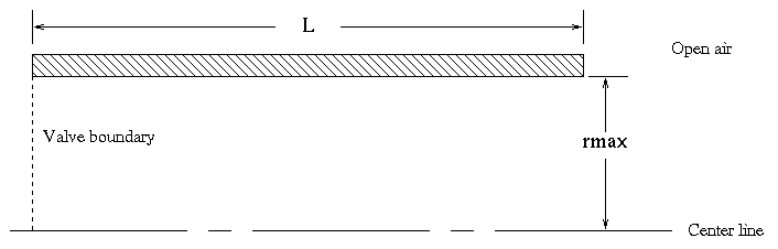
For example, consider a cylindrical pipe of length L with a valve on one end and open on the other, as shown above. Initially, the air in the pipe is motionless, but at some time t=0 the valve is opened, increasing the pressure at the valve end of the pipe by dp. Since air (or water or any other fluid) flows from high pressure to low pressure, the air inside the pipe will begin to flow to try to "get out of the way" of the increased pressure. However, the air has a resistance to flowing, known as viscosity, which causes the air to "stick" to the inner surface of the pipe. This will lead to the formation of a thin structure known as a boundary layer near the inner surface of the pipe where the air's viscosity (which is normally quite small) cannot be neglected.
Analysis
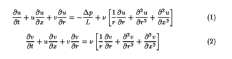
For the problem described above, the full Navier-Stokes equations are overkill. We can capture most of the essential features of the flow physics using a simplified set of equations known as the unsteady axisymmetric boundary layer equations:
Now these are still pretty nasty, because they involve partial derivatives (rates of change) of u and v with respect to time (t) and space (x and r). However, we can make things easier by making a grid where we want to know the solution, instead of trying to solve the equations for every possible point in space:
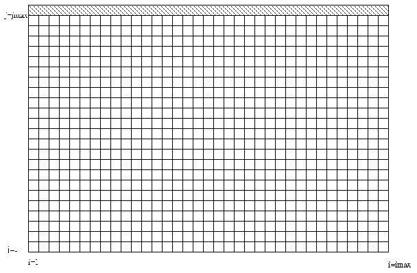
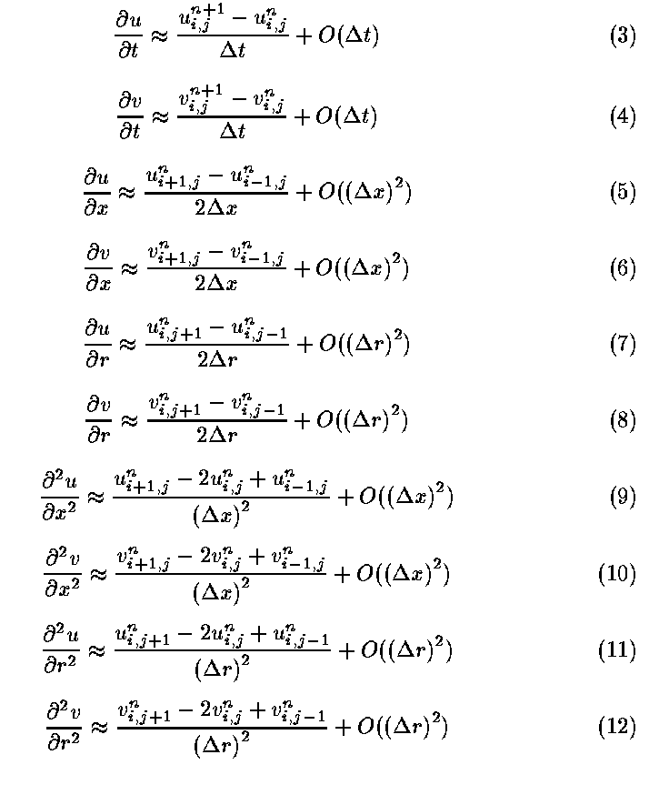
Once we have a grid, we can use a technique known as finite differencing to approximate the derivatives using the points on our grid:
Don't worry if this looks ugly and over your head, because it's about to get a whole lot simpler. If we're sneaky about the value of n we use in the some of the finite differences, we can reduce Equation (1) to the following:

If we consider all the u(i,j) for a given j value, this forms what's called a tridiagonal system of linear equations. Tridiagonal systems are well-known in linear algebra, and there are library routines on most of the supercomputers which can solve these systems very quickly.
Similarly, if we apply the same trick to Equation (2) that we used on Equation (1), we can get another tridiagonal system for v(i,j) at a given i value:

Initial Conditions
The initial conditions describe the state that the air inside the pipe is in before the valve is opened. If we assume that the air is not moving at all before the valve opens, then u(i,j) and v(i,j) can initially be set to zero everywhere.
Boundary Conditions
The boundaries of our domain have to be handled separately from the rest of the domain. This separate handling, known as the application of boundary conditions, is what makes the partial differential equations we saw above describe the particular geometry we are interested in. We can build part of the boundary conditions into the numerical method described above, but to be complete we 'll also want to build a separate routine for applying boundary conditions.
At the i=1 boundary, we have to apply what's known as an inflow boundary condition. Without going into the details of the mathematics, this means that we have to specify a value for one variable and extrapolate the other from the interior. Physically, what makes sense is to set u(1,j) equal to u(2,j) and v(1,j) to zero. In terms of our tridiagonal system above, the condition on u(1,j) means that A(1)=0, B(1)=1, C(1)=-1, and D(1)=0. The condition on v(1,j) will have to be applied in our boundary condition routine.
Similarly, we have to apply an outflow boundary condition at the i=imax boundary. For an outflow boundary condition, we need to extrapolate both u(imax,j) and v(imax,j) from the interior, so that unsteady disturbances are allowed to travel out of the domain. Thus, we would set u(imax,j) equal to u(imax-1,j) and v(imax,j) equal to v(imax-1,j). The condition on u(imax,j) means that A(imax)=1, B(imax)=-1, C(imax)=0, and D(imax)=0. As with the inflow conditions, the condition on v(imax,j) will have to be applied in our boundary condition routine.
At the j=1 boundary, we have to apply a symmetry or reflection boundary condition. This means that the resulting solution must be symmetric with respect to the j=1 line, which is the center line of the pipe. This results in conditions which are mathematically quite similar to those seem at the inflow boundary; u(i,1) must be set equal to u(i,2), while v(i,1) should be set to zero. The condition on v(i,1) means that E(1)=0, F(1)=1, G(1)=1, and H(1)=0. The condition on u(i,1) will have to be applied in our boundary condition routine.
Finally, at the j=jmax boundary, we have to apply a no-slip wall boundary condition. This means that the air sticks to the pipe surface because of friction. Of all the boundary conditions, this is probably the easiest to impose; u(i,jmax) and v(i.jmax) are simply set to zero. Similar to the symmetry condition above, the condition on v(i,jmax) means that E(jmax)=0, F(jmax)=1, G(jmax)=1, and H(jmax)=0. The condition on u(i,jmax) will again have to be applied in our boundary condition routine.
Outline
Here's an outline of what a program to solve the problem described above might look like:
- Declare variables and set constants
- Calculate x(i) and r(j) arrays
- Calculate initial values for u(i,j) and v(i,j) arrays
- For every time step
- For every j value between 2 and jmax-1
- Compute A(i), B(i), C(i), and D(i)
- Solve tridiagonal system for u(i,j)
- For every i value between 2 and imax-1
- Compute E(j), F(j), G(j), and H(j)
- Solve tridiagonal system for v(i,j)
- Apply boundary conditions
- Dump the solution to a file every so many iterations
- Clean up and terminate program
Requirements
The program should be written in a high level language such as Fortran-77, C, C++, Fortran-90, or Java. Fortran-77 and Fortran-90 have library routines for solving tridiagonal systems, so these are the preferred languages. The final program will be submitted electronically for evaluation; we will decide on a method to do this later. Graphics post-processing and animation will be done using the AVS graphics software.
Graphics Suggestions
There are several ways to graphically represent the behavior of the flow. The simplest, although not necessarily the most instructive, is to plot contours (lines of constant value) for either u or v. This can be a useful tool for debugging, but it does not give usually us much of an intuitive feel for the physical behavior being modeled.
A better way to visualize our results is to do what's called a hedgehog or vector plot. In this technique, we draw an arrow at each point in the direction of the velocity vector. We can encode additional information in the size and color of the arrow, such as the magnitude of the velocity or the vorticity (the degree to which the flow is rotating).
Another good way to visualize our results is to use the streamline technique. To do this, we seed the flow with an imaginary "particle" and trace the path that it follows as it travels downstream. This is much like the ribbons and smoke trails used in wind tunnels to visualize flow paths.
To look at the flow's behavior as it evolves over time, we can take images of either hedgehogs of streamlines at many time steps and show them in sequence, like the frames of a movie film. If we have enough images and show them rapidly, the result will (hopefully) be a smooth animation of the flow's evolution over time.
Extra Credit
Some things to look at if time allows:
- Normally, dp should be negative; it's the difference between the exit pressure and the inlet pressure, and we've been assuming that the inlet pressure is the higher of the two. What happens if you make dp positive (i.e. make the exit pressure higher than the inlet pressure)?
- Similarly, we've been assuming in this discussion that the viscosity nu is small (i.e. on the order of 0.01) and positive. While it doesn't make physical sense for nu to be negative, what happens if you make it 0.1? 1.0? 10.0?
- To reduce this problem to a rectangular rather than cylindrical pipe, you simply set the terms involving 1/r to zero. How does this affect the results?
ANIMATIONS
SI2004
SI2000
SI1998
Troy Baer is the OSC coordinator for the Pipe Flow project. Troy's office is in 420-6; please contact him to set up appointment(s) for consultation.
For assistance, write si-contact@osc.edu or call 614-292-0890.