Recorded on March 15, 2023.
Getting Started
What can OSC do for you? OSC's high performance computing, secure data storage and technical expertise can help advance research, accelerate business innovation and support classroom instruction.
Our comprehensive services guide provides an overview of our resources and how you can use them.
- Cluster computing: OSC offers three supercomputer clusters – Pitzer, Cardinal, and Ascend – that all support GPU computing.
- Research data storage: Clients can make use of work-area and supplemental storage during projects as well as long-term storage of data. Transfer files through our OnDemand platform or Globus subscription.
- Software: We provide a variety of software applications to support all aspects of scientific research. Ohio researchers may access licenses for some software packages through our statewide software program.
- Research software engineering: Our staff members can provide expert consultation on topics such as computing languages, programming models, numerical libraries and development tools for parallel/threaded computing and data analysis.
- Data analytics and machine learning: Our hardware and software offerings can accommodate the intensive workloads of data analytics and machine learning work.
- Dependability: The State of Ohio Computer Center, home of our computing clusters, provides security, climate control and fully redundant systems designed to keep OSC online at all times.
- Education: Faculty and students can learn about high performance computing through our webinars, workshops and how-to guides. Classroom accounts are available to instructors seeking to incorporate HPC work into courses.
How does the academic community use OSC?
Faculty at Ohio higher education institutions use OSC to conduct original research in fields ranging from engineering and medicine to plant biology and political science. Our extensive collection of case studies shows the breadth of research work underway, how graduate and undergraduate students are gaining critical HPC experience, and how academic clients make use of the wide variety of services and expert support that OSC provides.
How does the commercial and nonprofit community use OSC?
Commercial and nonprofit clients across the United States use OSC for research, simulations, development and testing of products. Our extensive collection of case studies offers examples of this work, including clients involved with pharmaceutical drug development, the simulation of how fluid dynamics impact vehicle performance, the study of factors impacting oil and gas pipeline corrosion, and the advancement of weather-forecasting technology.
What does it cost to use OSC?
As an academic computing resource for the State of Ohio, OSC is always free for Ohio classroom usage, and academic researchers in Ohio qualify for credits that largely or completely offset fees. Commercial and nonprofit clients purchase services at set rates. Find more details about our cost structure.
What training or client support does OSC offer?
OSC provides a variety of training and support options for clients:
- Read our new user guide
- Take one of our self-paced courses on how to use our HPC resources for research and classroom instruction
- Sign up for virtual help sessions, workshops, or webinars
- Visit our training page to view a full list of opportunities
Ready to take the next step?
Interested talking to our staff about OSC’s resources and services? Please contact us at start@osc.edu. (Please note that this is NOT a technical support channel. If you have a login ID already, please visit the Service Center for support.)
Ready to get started now?
Request a new login ID for an existing project
New User Resource Guide
Getting Started at OSC
This guide was created for new users of OSC.
It explains how to use OSC from the very beginning of the process, from creating an account right up to using resources at OSC.
OSC account setup
The first step is to make sure that you have an OSC username.
There are multiple ways to start this process.
You can sign up at MyOSC or be invited to use OSC via email.
Make sure to select the PI checkbox if you are a PI at your institution and want to start your own project at OSC.
After creating an account at MyOSC, you may not be able to log into OSC using OnDemand or an SSH client. If you do not have access to a project, you would get an "invalid credentials" message, although the credentials are correct. Sometimes OSC administrators need to approve your username if your institution is not recognized in our database.
Contact OSC Help with questions.
Contact OSC Help with questions.
Email notifications from OSC
As soon as you register for an account with OSC, you will start receiving automated emails from MyOSC. These include password expiration emails, access to project(s), etc. These are sent from "no-reply@osc.edu." All folders should be checked, including spam/junk. If you did not receive this email, please contact OSC Help.
OSC will also add you to our mailing list within a month of your account being opened. Emails will be sent from oschelp@osc.edu for system notices, monthly newsletters, event updates, etc. This information can also be found on our events page and known issues page.
Finally, we may notify clients through ServiceNow, our internal ticketing and monitoring system. These notices will come from the OH-TECH Service Desk, support@oh-tech.org.
Project and user management
Creating a project
Only users with PI status are able to create a project. See how to request PI status in manage profile information. Follow the instructions in creating projects and budgets to create a new project.
Adding new or existing users to a project
Once a project is created, the PI should add themselves to it and any others that they want to permit to use OSC resources under their project.
Refer to adding/inviting users to a project for details on how to do this.
Reuse an existing project
If there was already a project that you would like to reuse, follow the same instructions as found in creating projects and budget, but skip to the budget creation section.
These instructions are the same for projects which are restricted. Creating a new budget and getting it activated or approved will set the project to active.
Costs of OSC resources
If there are questions about the cost, refer to service costs.
Generally, an Ohio academic PI can create a budget for $1,000 on a project and use the annual $1,000 credit offered to Ohio academic PIs. Review service cost terms for explanations of budgets and credits at OSC.
See the complete MyOSC documentation in our Client Portal here. The OSCusage command can also provide useful details.
Classroom project support
OSC supports classrooms by making it simpler for students to use OSC resources through a customizable OnDemand interface at class.osc.edu
Visit the OSC classroom resource guide and contact oschelp@osc.edu if you want to discuss the options there.
There will be no charges for classroom projects.
Transfer files to/from OSC systems
There are a few options for transferring files between OSC and other systems.
OnDemand file explorer
Using the OnDemand file explorer is the quickest option to get started. Just log into ondemand.osc.edu and click "File Explorer" from the navigation bar at the top of the page. From there you can upload/download files and directories.
Users cannot access ondemand.osc.edu unless they have an active OSC account and have been added to at least one project. Refer to the above sections which cover this.
This is a simple option, but for files or directories that are very large, it may not be best. See other options below in this case.
SFTP client software
Local software can be used to connect to OSC for downloading and uploading files.
There are quite a few options for this, and OSC does not have a preference for which one you use.
The general guidance for all of them is to connect to host sftp.osc.edu using port 22.
Globus
Using Globus is recommended for users that frequently need to transfer many large files/dirs.
We have documentation detailing how to connect to our OSC endpoint in Globus and how to set up a local endpoint on your machine with Globus.
Request extra storage for a project
Storage can be requested for a project that is larger than the standard offered by home directories.
On the project details page, submit a "Request Storage Change" and a ticket will be created for OSC staff to create the project space quota.
Make sure that the cost of storage is understood prior to sending the request.
See service costs for details.
See service costs for details.
Getting started using OSC
Finally, after the above setup, you can start using OSC resources. Usually you have some setup that needs to be performed before you can really start using OSC, like creating a custom environment, gaining access to preinstalled software or installing software to your home directory that is not already available.
Interactive desktop session
The best place to start is by visiting ondemand.osc.edu, logging in and starting an interactive desktop session.
Look for the navigation bar at the top of the page and select Interactive Apps, then choose a Desktop.
Notice that there are a lot of fields, but the most important ones, for now, are cores and the number of hours.
Try using only a single core at first, until you are more familiar with the system and can decide when more cores will be needed.
Other interactive apps
If there is specific software in the Interactive Apps list that you want to use, then go ahead and start a session with it. Just remember to change the cores to one until you understand what you need.
Getting to a terminal without starting a desktop session
A terminal session can also be started in OnDemand by clicking Clusters, then selecting a Shell Access.
In this terminal you can perform the needed commands in the below sections on environment setup and software use/installation.
You can choose to log into OSC with any ssh client available. Make sure to use either cardinal.osc.edu or pitzer.osc.edu as the hostname to connect to.
Environment setup to install packages for different programming languages
Some of the common programming languages for which users need an environment set up are python and R.
See add python packages with conda or R software for details.
There are other options, so please browse the OSC software listing.
OSC managed software
All the software already available at OSC can be found in the software listing.
Each page has some information on how to use the software from a command line. If you are unfamiliar with the command line in Linux, then try reviewing some Linux tutorials.
For now, try to get comfortable with moving to different directories on the filesystem, creating and editing files, and using the module commands from the software pages.
Install software not provided by OSC
Software not already installed on OSC systems can be installed locally to one's home directory without admin privileges. Try reviewing locally installing software at OSC.
Batch system basics
After getting set up at OSC and understanding the use of interactive sessions, you should start looking into how to utilize the batch system to have your software run programmatically.
The benefits of the batch system are that a user can submit what we call a job (a request to reserve resources) and have the job execute from start to finish without any interaction by the user.
A good place to start is by reviewing job scripts.
OnDemand job composer
OnDemand provides a convenient method for editing and submitting jobs in the job composer.
It can be used by logging into ondemand.osc.edu and clicking Jobs at the top and then Job Composer. A short help message should be shown on basic usage.
Training
OSC offers periodic training both at our facility and at universities across the state on a variety of topics. Additionally, we will partner with other organizations to enable our users to access additional training resources.
We are currently in the process of updating our training strategy and documents. If you are interested in having us come to your campus to provide training, please contact OSC Help. You can also contact us if there is a specific training need you would like to see us address.
To get an introduction to HPC, see our HPC Basics page.
To learn more about using the command line, see our UNIX Basics page.
For detailed instructions on how to perform tasks on our systems, check out HOWTO articles.
Still Need Help?
Before contacting OSC Help, please check to see if your question is answered in either the FAQ or the Knowledge Base. Many of the questions asked by both new and experienced OSC users are answered on these web pages.
If you still cannot solve your problem, please do not hesitate to contact OSC Help:
Phone: (614) 292-1800
Email: oschelp@osc.edu
Submit your issue online
Schedule virtual consultation
Basic and advanced support is available Monday through Friday, 9 a.m.– 5 p.m., except for these listed holidays.
We recommend following HPCNotices on X to get up-to-the-minute information on system outages and important operations-related updates.
Documentation Attachment:
Supercomputer:
HPC Basics
New! Online Training Courses
Check out our new online training courses for an introduction to OSC services. You can get more information on the OSC Training page.
Overview
HPC, or High Performance Computing, generally refers to aggregating computing resources together in order to perform more computing operations at once.
Basic definitions
- Core (processor) - A single unit that executes a single chain of instructions.
- Node - a single computer or server.
- Cluster - many nodes connected together which are able to coordinate between themselves.
HPC Workflow
Using HPC is a little different from running programs on your desktop. When you login you’ll be connected to one of the system’s “login nodes”. These nodes serve as a staging area for you to marshal your data and submit jobs to the batch scheduler. Your job will then wait in a queue along with other researchers' jobs. Once the resources it requires become available, the batch scheduler will then run your job on a subset of our hundreds of “compute nodes”. You can see the overall structure in the diagram below.
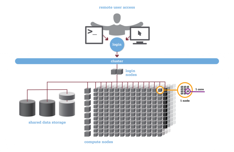
HPC Citizenship
An important point about the diagram above is that OSC clusters are a collection of shared, finite resources. When you connect to the login nodes, you are sharing their resources (CPU cycles, memory, disk space, network bandwidth, etc.) with a few dozen other researchers. The same is true of the file servers when you access your home or project directories, and can even be true of the compute nodes.
For most day-to-day activities you should not have to worry about this, and we take precautions to limit the impact that others might have on your experience. That said, there are a few use cases that are worth watching out for:
-
The login nodes should only be used for light computation; any CPU- or memory-intensive operations should be done using the batch system. A good rule of thumb is that if you wouldn't want to run a task on your personal desktop because it would slow down other applications, you shouldn't run it on the login nodes. (See also: Interactive Jobs.)
-
I/O-intensive jobs should copy their files to fast, temporary storage, such as the local storage allocated to jobs or the Scratch parallel filesystem.
-
When running memory-intensive or potentially unstable jobs, we highly recommend requesting whole nodes. By doing so you prevent other users jobs from being impacted by your job.
-
If you request partial nodes, be sure to consider the amount of memory available per core. (See: HPC Hardware.) If you need more memory, request more cores. It is perfectly acceptable to leave cores idle in this situation; memory is just as valuable a resource as processors.
In general, we just encourage our users to remember that what you do may affect other researchers on the system. If you think something you want to do or try might interfere with the work of others, we highly recommend that you contact us at oschelp@osc.edu.
Getting Connected
There are two ways to connect to our systems. The traditional way will require you to install some software locally on your machine, including an SSH client, SFTP client, and optionally an X Windows server. The alternative is to use our zero-client web portal, OnDemand.
OnDemand Web Portal
OnDemand is our "one stop shop" for access to our High Performance Computing resources. With OnDemand, you can upload and download files, create, edit, submit, and monitor jobs, run GUI applications, and connect via SSH, all via a web broswer, with no client software to install and configure.
You can access OnDemand by pointing a web browser to ondemand.osc.edu. Documentation is available here. Any newer version of a common web browser should be sufficient to connect.
Using Traditional Clients
Required Software
In order to use our systems, you'll need two main pieces of software: an SSH client and an SFTP client.
SSH ("Secure Shell") clients allow you to open a command-line-based "terminal session" with our clusters. We recommend the following options:
- PuTTY: A simple, open-source client for Windows.
- Secure Shell for Google Chrome: A free, HTML5-based SSH client for Google Chrome.
- ssh: The command-line utility ssh comes pre-installed on OS X and most Linux systems.
SFTP ("SSH File Transfer Protocol") clients allow you transfer files between your workstation and our shared filesystem in a secure manner. We recommend the following applications:
- FileZilla: A high-performance open-source client for Windows, Linux, and OS X. A guide to using FileZilla is available here (external).
- CyberDuck: A high quality free client for Windows and OS X.
- sftp: The command-line utility sftp comes pre-installed on OS X and most Linux systems.
A third, optional piece of software you might want to install is an X Windows server, which will be necessary if you want to run graphical, windowed applications like MATLAB. We recommend the following X Windows servers:
- Xming: Xming offers a free version of their X Windows server for Microsoft Windows systems.
- X-Win32: StarNet's X-Win32 is a commercial X Windows server for Microsoft Windows systems. They offer a free, thirty-day trial.
- X11.app/XQuartz: X11.app, an Apple-supported version of the open-source XQuartz project, is freely available for OS X.
Connecting via SSH
The primary way you'll interact with the OSC clusters is through the SSH terminal. See our supercomputing environments for the hostnames of our current clusters.
Once you've established an SSH connection, you will be presented with some informational text about the cluster you've connected to followed by a UNIX command prompt. For a brief discussion of UNIX command prompts and what you can do with them, see this guide.
Transferring Files
To transfer files, use your preferred SFTP client to connect to:
sftp.osc.edu
You may see warning message including SSH key fingerprint. Verify that the fingerprint in the message matches one of the SSH key fingerprint listed here, then type yes.
Since process times are limited on the login nodes, trying to transfer large files directly to login nodes (like cardinal.osc.edu) may terminate partway through. The sftp.osc.edu is specially configured to avoid this issue, and so we recommend it for all your file transfers.
Note: The sftp.osc.edu host is not connected to the scheduler, so you cannot submit jobs from this host. Use of this host for any purpose other than file transfer is not permitted.
Firewall Configuration
See our Firewall and Proxy Settings page for information on how to configure your firewall to allow connection to and from OSC.
Setting up X Windows (Optional)
With an X Windows server you will be able to run graphical applications on our clusters that display on your workstation. To do this, you will need to launch your X Windows server before connecting to our systems. Then, when setting up your SSH connection, you will need to be sure to enable "X11 Forwarding".
For users of the command-line ssh client, you can do this by adding the "-X" option. For example, the below will connect to the Pitzer cluster with X11 forwarding:
$ ssh -X username@pitzer.osc.edu
If you are connecting with PuTTY, the checkbox to enable X11 forwarding can be found in the connections pane under "Connections → SSH → X11".
For other SSH clients, consult their documentation to determine how to enable X11 forwarding.
NOTE: The X-Windows protocol is not a high-performance one. Depending on your system and Internet connection, X Windows applications may run very slowly, even to the point of being unusable. If you find this to be the case and graphical applications are a necessity for your work, please contact OSC Help to discuss alternatives.
Service:
Budgets and Accounts
The Ohio Supercomputer Center provides services to clients from a variety of types of organizations. The methods for gaining access to the systems are different between Ohio academic institutions and everyone else.
Ohio academic clients
Primarily, our users are Ohio-based and academic, and the vast majority of our resources will continue to be consumed by Ohio-based academic users. See the "Ohio Academic Fee Model FAQ" section on our service costs webpage.
Other clients
Other users (business, non-Ohio academic, nonprofit, hospital, etc.) interested in using Center resources may purchase services at a set rate available on our price list. Expert consulting support is also available.
Other computing centers
For users interested in gaining access to larger resources, please contact OSC Help. We can assist you in applying for resources at an NSF or XSEDE site.
Managing an OSC project
Once a project has been created, the PI can create accounts for users by adding them through the client portal. Existing users can also be added. More information can be found on the Project Menu documentation page.
I need additional resources for my existing project and/or I received an email my allocation is exhausted
If an academic PI wants a new project or to update the budget balance on an existing project(s), please see our creating projects and budget documentation.
I wish to use OSC to support teaching a class
We provide special classroom projects for this purpose and at no cost. You may use the client portal after creating an account. The request will need to include a syllabus or a similar document.
I don't think I fit in the above categories
Please contact us in order to discuss options for using OSC resources.
Applying for Academic Accounts
The procedures described enable services to be available to approved projects conducted by eligible principal investigators (PIs) at Ohio academic institutions. An eligible PI must have a full-time appointment at a college, a university, or a research organization administered by an Ohio academic institution (i.e., be a full-time, permanent academic researcher or tenure-track faculty member or an emeritus professor at an Ohio college or university). Students, post-doctoral fellows, visiting scientists, and others who wish to use the facilities may be authorized users on projects headed by an eligible PI. Once a PI has received an OSC Academic Account, he/she can log into the Client Portal (https://my.osc.edu) to add new authorized user(s) to a project.
OSC's online account application is part of an electronic system that leads you through the process step by step. Before you begin to fill in the application form, especially if you are new to the process, look at the Account Application Help pages.
If you need assistance, please contact OSC Help.
Applying for Commercial Access
Researchers from commercial organizations who wish to use the OSC's resources, please contact OSC Sales.
Letter of Support for Outside Funding Proposals
OSC will provide a letter of support users can include with their account proposals for outside funding, such as from the National Science Foundation and the National Institutes of Health. This letter details OSC's commitment to supporting research efforts of its users and the facilities and platforms we provide our users. [Note: This letter does not waive the normal OSC account application process; it merely states that OSC is willing to support such application.] Please provide a draft letter that complies with solicitation or funding agency requirements.
If you need assistance, please contact OSC Help.
Applying at NSF Centers
Researchers requiring additional computing resources, above what OSC can provide, should consider applying for allocations to utilize National Science Foundation Centers. For more information, please visit the NSF ACCESS website and/or the NAIRR website.
Acknowledging the Ohio Supercomputer Center
OSC requires acknowledgment in any publications or reports that result from projects supported by OSC accounts of resources. Please visit the OSC Citation page for more details.
UNIX Basics
OSC HPC resources use an operating system called "Linux", which is a UNIX-based operating system, first released on 5 October 1991. Linux is by a wide margin the most popular operating system choice for supercomputing, with over 90% of the Top 500 list running some variant of it. In fact, many common devices run Linux variant operating systems, including game consoles, tablets, routers, and even Android-based smartphones.
While Linux supports desktop graphical user interface configurations (as does OSC) in most cases, file manipulation will be done via the command line. Since all jobs run in batch will be non-interactive, they by definition will not allow the use of GUIs. Thus, we strongly suggest new users become comfortable with basic command-line operations, so that they can learn to write scripts to submit to the scheduler that will behave as intended. We have provided some tutorials explaining basics from moving about the file system, to extracting archives, to modifying your environment, that are available for self-paced learning.
Linux Command Line Fundamentals
This tutorial teaches you about the linux command line and shows you some useful commands. It also shows you how to get help in linux by using the man and apropos commands.
Linux Tutorial
This tutorial guides you through the process of creating and submitting a batch script on one of our compute clusters. This is a linux tutorial which uses batch scripting as an example, not a tutorial on writing batch scripts. The primary goal is not to teach you about batch scripting, but for you to become familiar with certain linux commands that can be used either in a batch script or at the command line. There are other pages on the OSC web site that go into the details of submitting a job with a batch script.
Linux Shortcuts
This tutorial shows you some handy time-saving shortcuts in linux. Once you have a good understanding of how the command line works, you will want to learn how to work more efficiently.
Tar Tutorial
This tutorial shows you how to download tar (tape archive) files from the internet and how to deal with large directory trees of files.
Service:
Linux Command Line Fundamentals
Description
This tutorial teaches you about the linux command line and shows you some useful commands. It also shows you how to get help in linux by using the man and apropos commands.
For more training and practice using the command line, you can find many great tutorials. Here are a few:
https://www.learnenough.com/command-line-tutorial
https://cvw.cac.cornell.edu/Linux/
http://www.ee.surrey.ac.uk/Teaching/Unix/
https://www.udacity.com/course/linux-command-line-basics--ud595
More Advanced:
http://moo.nac.uci.edu/~hjm/How_Programs_Work_On_Linux.html
Prerequisites
None.
Introduction
Unix is an operating system that comes with several application programs. Other examples of operating systems are Microsoft Windows, Apple OS and Google's Android. An operating system is the program running on a computer (or a smartphone) that allows the user to interact with the machine -- to manage files and folders, perform queries and launch applications. In graphical operating systems, like Windows, you interact with the machine mainly with the mouse. You click on icons or make selections from the menus. The Unix that runs on OSC clusters gives you a command line interface. That is, the way you tell the operating system what you want to do is by typing a command at the prompt and hitting return. To create a new folder you type mkdir. To copy a file from one folder to another, you type cp. And to launch an application program, say the editor emacs, you type the name of the application. While this may seem old-fashioned, you will find that once you master some simple concepts and commands you are able to do what you need to do efficiently and that you have enough flexibility to customize the processes that you use on OSC clusters to suit your needs.
Common Tasks on OSC Clusters
What are some common tasks you will perform on OSC clusters? Probably the most common scenario is that you want to run some of the software we have installed on our clusters. You may have your own input files that will be processed by an application program. The application may generate output files which you need to organize. You will probably have to create a job script so that you can execute the application in batch mode. To perform these tasks, you need to develop a few different skills. Another possibility is that you are not just a user of the software installed on our clusters but a developer of your own software -- or maybe you are making some modifications to an application program so you need to be able to build the modified version and run it. In this scenario you need many of the same skills plus some others. This tutorial shows you the basics of working with the Unix command line. Other tutorials go into more depth to help you learn more advanced skills.
The Kernel and the Shell
You can think of Unix as consisting of two parts -- the kernel and the shell. The kernel is the guts of the Unix operating system -- the core software running on a machine that performs the infrastructure tasks like making sure multiple users can work at the same time. You don't need to know anything about the kernel for the purposes of this tutorial. The shell is the program that interprets the commands you enter at the command prompt. There are several different flavors of Unix shells -- Bourne, Korn, Cshell, TCshell and Bash. There are some differences in how you do things in the different shells, but they are not major and they shouldn't show up in this tutorial. However, in the interest of simplicity, this tutorial will assume you are using the Bash shell. This is the default shell for OSC users. Unless you do something to change that, you will be running the Bash shell when you log onto Owens or Pitzer.
The Command Prompt
The first thing you need to do is log onto one of the OSC clusters, Owens or Pitzer. If you do not know how to do this, you can find help at the OSC home page. If you are connecting from a Windows system, you need to download and setup the OSC Starter Kit which you can find here. If you are connecting from a Mac or Linux system, you will use ssh. To get more information about using ssh, go to the OSC home page, hold your cursor over the "Supercomputing" menu in the main blue menu bar and select "FAQ." This should help you get started. Once you are logged in look for the last thing displayed in the terminal window. It should be something like
-bash-3.2$
with a block cursor after it. This is the command prompt -- it's where you will see the commands you type in echoed to the screen. In this tutorial, we will abbreviate the command prompt with just the dollar sign - $. The first thing you will want to know is how to log off. You can log off of the cluster by typing "exit" then typing the <Enter> key at the command prompt:
$ exit <Enter>
For the rest of this tutorial, when commands are shown, the <Enter> will be omitted, but you must always enter <Enter> to tell the shell to execute the command you just typed.
First Simple Commands
So let's try typing a few commands at the prompt (remember to type the <Enter> key after the command):
$ date

$ cal

$ finger

$ who

$ whoami

$ finger -l
That last command is finger followed by a space then a minus sign then the lower case L. Is it obvious what these commands do? Shortly you will learn how to get information about what each command does and how you can make it behave in different ways. You should notice the difference between "finger" and "finger -l" -- these two commands seem to do similar things (they give information about the users who are logged in to the system) but they print the information in different formats. try the two commands again and examine the output. Note that you can use the scroll bar on your terminal window to look at text that has scrolled off the screen.
man
The "man" command is how you find out information about what a command does. Type the following command:
$ man
It's kind of a smart-alecky answer you get back, but at least you learn that "man" is short for "manual" and that the purpose is to print the manual page for a command. Before we start looking at manual pages, you need to know something about the way Unix displays them. It does not just print the manual page and return you to the command prompt -- it puts you into a mode where you are interactively viewing the manual page. At the bottom of the page you should see a colon (:) instead of the usual command prompt (-bash-3.2$). You can move around in the man page by typing things at the colon. To exit the man page, you need to type a "q" followed by <Enter>. So try that first. Type
$ man finger
then at the colon of the man page type
: q
You do not have to type <Enter> after the "q" (this is different from the shell prompt.) You should be back at the shell prompt now. Now let's go through the man page a bit. Once again, type
$ man finger
Now instead of just quitting, let's look at the contents of the man page. The entire man page is probably not displayed in your terminal. To scroll up or down, use the arrow keys or the <Page Up> and <Page Down> keys of the keyboard. The <Enter> and <Space> keys also scroll. Remember that "q" will quit out of the man page and get you back to the shell prompt.
The first thing you see is a section with the heading "NAME" which displays the name of the command and a short summary of what it does. Then there is a section called "SYNOPSIS" which shows the syntax of the command. In this case you should see
SYNOPSIS

     finger [-lmsp] [user ...] [user@host ...]
Remember how "finger" and "finger -l" gave different output? The [-lmsp] tells you that you can use one of those four letters as a command option -- i.e., a way of modifying the way the command works. In the "DESCRIPTION" section of the man page you will see a longer description of the command and an explanation of the options. Anything shown in the command synopsis which is contained within square brackets ([ ]) is optional. That's why it is ok to type "finger" with no options and no user. What about "user" -- what is that? To see what that means, quit out of the man page and type the following at the command prompt:
$ whoami
Let's say your username is osu0000. Then the result of the "whoami" command is osu0000. Now enter the following command (but replace osu0000 with your username):
$ finger osu0000
You should get information about yourself and no other users. You can also enter any of the usernames that are output when you enter the "finger" command by itself. The user names are in the leftmost column of output. Now try
$ finger -l osu0000

$ finger -lp osu0000

$ finger -s osu0000 osu0001
For the last command, use your username and the username of some other username that shows up in the output of the "finger" command with no arguments.
Note that a unix command consists of three parts:
- command
- option(s)
- argument(s)
You don't necessarily have to enter an argument (as you saw with the "finger" command) but sometimes a command makes no sense without an argument so you must enter one -- you saw this with the "man" command. Try typing
$ man man
and looking briefly at the output. One thing to notice is the synopsis -- there are a lot of possible options for the "man" command, but the last thing shown in the command synopsis is "name ..." -- notice that "name" is not contained in square brackets. This is because it is not optional -- you must enter at least one name. What happens if you enter two names?
$ man man finger
The first thing that happens is you get the man page for the "man" command. What happens when you quit out of the man page? You should now get the man page for the "finger" command. If you quit out of this one you will be back at the shell prompt.
Combining Commands
You can "pipe" the output of one command to another. First, let's learn about the "more" command:
$ man more
Read the "DESCRIPTION" section -- it says that more is used to page through text that doesn't fit on one screen. It also recommends that the "less" command is more powerful. Ok, so let's learn about the "less" command:
$ man less
You see from the description that "less" also allows you to examine text one screenful at a time. Does this sound familiar? The "man" command actually uses the "less" command to display its output. But you can use the "less" command yourself. If you have a long text file named "foo.txt" you could type
$ less foo.txt
and you would be able to examine the contents of the file one screen at a time. But you can also use "less" to help you look at the output of a command that prints more than one screenful of output. Try this:
$ finger | less
That's "finger" followed by a space followed by the vertical bar (shifted backslash on most keyboards) followed by a space followed by "less" followed by <Enter>. You should now be looking at the output of the "finger" command in an interactive fashion, just as you were looking at man pages. Remember, to scroll use the arrow keys, the <Page Up> and <Page Down> keys, the <Enter> key or the space bar; and to quit, type "q".
Now try the following (but remember to replace "osu0000" with your actual username):
$ finger | grep osu0000
The "grep" command is Unix's command for searching. Here you are telling Unix to search the output of the "finger" command for the text "osu0000" (or whatever your username is.)
If you try to pipe the output of one command to a second command and the second is a command which works with no arguments, you won't get what you expect. Try
$ whoami | finger
You see that it does not give the same output as
$ finger osu0000
(assuming "whoami" returns osu0000.)
In this case what you can do is the following:
$ finger `whoami`
That's "finger" space backquote "whoami" backquote. The backquote key is to the left of the number 1 key on a standard keyboard.
apropos
Enter the following command:
$ man apropos
As you can see, the apropos searches descriptions of commands and finds commands whose descriptions match the keyword you entered as the argument. That means it outputs a list of commands that have something to do with the keyword you entered. Try this
$ apropos
Ok, you need to enter an argument for the "apropos" command.
So try
$ apropos calendar
Now you see that among the results are two commands -- "cal" and "difftime" that have something to do with the keyword "calendar."
Linux Tutorial
Description
This tutorial guides you through the process of creating and submitting a batch script on one of our compute clusters. This is a linux tutorial which uses batch scripting as an example, not a tutorial on writing batch scripts. The primary goal is not to teach you about batch scripting, but for you to become familiar with certain linux commands. There are other pages on the OSC web site that go into the details of submitting a job with a batch script.
Prerequisites
- Familiarity with a text editor (emacs, nano, vim)
- Basic understanding of the unix command line
- Linux Command Line Fundamentals tutorial
Goals
- Create subdirectories to organize information
- Create a batch script with a text editor
- Submit a job
- Check on the progress of the job
- Change the permissions of the output files
- Get familiar with some common unix commands
Step 1 - Organize your directories
When you first log in to our clusters, you are in your home directory. For the purposes of this illustration, we will pretend you are user osu0001 and your project code is PRJ0001, but when you try out commands you must use your own username and project code.
$ pwd
/users/PRJ0001/osu0001
Note: you will see your user name and a different number after the /users.
It's a good idea to organize your work into separate directories. If you have used Windows or the Mac operating system, you may think of these as folders. Each folder may contain files and subfolders. The subfolders may contain other files and subfolders of their own. In linux we use the term "directory" instead of "folder." Use directories to organize your work.
Type the following four lines and take note of the output after each one:
$ touch foo1
$ touch foo2
$ ls
$ ls -l
$ ls -lt
$ ls -ltr
The "
touch" command just creates an empty file with the name you give it.You probably already know that the ls command shows the contents of the current working directory; that is, the directory you see when you type pwd. But what is the point of the "
-l", "-lt" or "-ltr"? You noticed the difference in the output between just the "ls" command and the "ls -l" command.Most unix commands have options you can specify that change the way the command works. The options can be specified by the "
-" (minus sign) followed by a single letter. "ls -ltr" is actually specifying three options to the ls command.l: I want to see the output in long format -- one file per line with some interesting information about each filet: sort the display of files by when they were last modified, most-recently modified firstr: reverse the order of display (combined with -t this displays the most-recently modified file last -- it should be BatchTutorial in this case.)I like using "
ls -ltr" because I find it convenient to see the most recently modified file at the end of the list.Now try this:
$ mkdir BatchTutorial
$ ls -ltr
The "
mkdir" command makes a new directory with the name you give it. This is a subfolder of the current working directory. The current working directory is where your current focus is in the hierarchy of directories. The 'pwd' command shows you are in your home directory:$ pwd /users/PRJ0001/osu0001
Now try this:
$ cd BatchTutorial
$ pwd
What is the output of '
pwd' now? "cd" is short for "change directory" -- think of it as moving you into a different place in the hierarchy of directories. Now do$ cd .. $ pwd
Where are you now?
Step 2 -- Get familiar with some more unix commands
Try the following:
$ echo where am I?
$ echo I am in `pwd`
$ echo my home directory is $HOME
$ echo HOME
$ echo this directory contains `ls -l`
These examples show what the echo command does and how to do some interesting things with it. The `pwd` means the result of issuing the command pwd. HOME is an example of an environment variable. These are strings that stand for other strings. HOME is defined when you log in to a unix system. $HOME means the string the variable HOME stands for. Notice that the result of "echo HOME" does not do the substitution. Also notice that the last example shows things don't always get formatted the way you would like.
Some more commands to try:
$ cal
$ cal > foo3
$ cat foo3
$ whoami
$ date
Using the ">" after a command puts the output of the command into a file with the name you specify. The "cat" command prints the contents of a file to the screen.
Two very important UNIX commands are the cp and mv commands. Assume you have a file called foo3 in your current directory created by the "cal > foo3" command. Suppose you want to make a copy of foo3 called foo4. You would do this with the following command:
$ cp foo3 foo4
$ ls -ltr
Now suppose you want to rename the file 'foo4' to 'foo5'. You do this with:
$ mv foo4 foo5
$ ls -ltr
'mv' is short for 'move' and it is used for renaming files. It can also be used to move a file to a different directory.
$ mkdir CalDir
$ mv foo5 CalDir
$ ls
$ ls CalDir
Notice that if you give a directory with the "ls" command is shows you what is in that directory rather than the current working directory.
Now try the following:
$ ls CalDir
$ cd CalDir
$ ls
$ cd ..
$ cp foo3 CalDir
$ ls CalDir
Notice that you can use the "cp" command to copy a file to a different directory -- the copy will have the same name as the original file. What if you forget to do the mkdir first?
$ cp foo3 FooDir
Now what happens when you do the following:
$ ls FooDir
$ cd FooDir
$ cat CalDir
$ cat FooDir
$ ls -ltr
CalDir is a directory, but FooDir is a regular file. You can tell this by the "d" that shows up in the string of letters when you do the "ls -ltr". That's what happens when you try to cp or mv a file to a directory that doesn't exist -- a file gets created with the target name. You can imagine a scenario in which you run a program and want to copy the resulting files to a directory called Output but you forget to create the directory first -- this is a fairly common mistake.
Step 3 -- Environment Variables
Before we move on to creating a batch script, you need to know more about environment variables. An environment variable is a word that stands for some other text. We have already seen an example of this with the variable HOME. Try this:
$ MY_ENV_VAR="something I would rather not type over and over"
$ echo MY_ENV_VAR
$ echo $MY_ENV_VAR
$ echo "MY_ENV_VAR stands for $MY_ENV_VAR"
You define an environment variable by assigning some text to it with the equals sign. That's what the first line above does. When you use '$' followed by the name of your environment variable in a command line, UNIX makes the substitution. If you forget the '$' the substitution will not be made.
There are some environment variables that come pre-defined when you log in. Try using 'echo' to see the values of the following variables: HOME, HOSTNAME, SHELL, TERM, PATH.
Now you are ready to use some of this unix knowledge to create and run a script.
Step 4 -- Create and run a script
Before we create a batch script and submit it to a compute node, we will do something a bit simpler. We will create a regular script file that will be run on the login node. A script is just a file that consists of unix commands that will run when you execute the script file. It is a way of gathering together a bunch of commands that you want to execute all at once. You can do some very powerful things with scripting to automate tasks that are tedious to do by hand, but we are just going to create a script that contains a few commands we could easily type in. This is to help you understand what is happening when you submit a batch script to run on a compute node.
Use a text editor to create a file named "tutorial.sh" which contains the following text (note that with emacs or nano you can use the mouse to select text and then paste it into the editor with the middle mouse button):
$ nano tutorial.sh
echo ----
echo Job started at `date`
echo ----
echo This job is working on node `hostname`

SH_WORKDIR=`pwd`
echo working directory is $SH_WORKDIR
echo ----
echo The contents of $SH_WORKDIR
ls -ltr
echo
echo ----
echo
echo creating a file in SH_WORKDIR
whoami > whoami-sh-workdir

SH_TMPDIR=${SH_WORKDIR}/sh-temp
mkdir $SH_TMPDIR
cd $SH_TMPDIR
echo ----
echo TMPDIR IS `pwd`
echo ----
echo wait for 12 seconds
sleep 12
echo ----
echo creating a file in SH_TMPDIR
whoami > whoami-sh-tmpdir

# copy the file back to the output subdirectory
cp ${SH_TMPDIR}/whoami-sh-tmpdir ${SH_WORKDIR}/output

cd $SH_WORKDIR

echo ----
echo Job ended at `date`
To run it:
$ chmod u+x tutorial.sh
$ ./tutorial.sh
Look at the output created on the screen and the changes in your directory to see what the script did.
Step 5 -- Create and run a batch job
Use your favorite text editor to create a file called tutorial.pbs in the BatchTutorial directory which has the following contents (remember, you can use the mouse to cut and paste text):
#PBS -l walltime=00:02:00
#PBS -l nodes=1:ppn=1
#PBS -N foobar
#PBS -j oe
#PBS -r n

echo ----
echo Job started at `date`
echo ----
echo This job is working on compute node `cat $PBS_NODEFILE`

cd $PBS_O_WORKDIR
echo show what PBS_O_WORKDIR is
echo PBS_O_WORKDIR IS `pwd`
echo ----
echo The contents of PBS_O_WORKDIR:
ls -ltr
echo
echo ----
echo
echo creating a file in PBS_O_WORKDIR
whoami > whoami-pbs-o-workdir

cd $TMPDIR
echo ----
echo TMPDIR IS `pwd`
echo ----
echo wait for 42 seconds
sleep 42
echo ----
echo creating a file in TMPDIR
whoami > whoami-tmpdir

# copy the file back to the output subdirectory
pbsdcp -g $TMPDIR/whoami-tmpdir $PBS_O_WORKDIR/output

echo ----
echo Job ended at `date`
To submit the batch script, type
$ qsub tutorial.pbs
Use
qstat -u [username] to check on the progress of your job. If you see something like this
$ qstat -u osu0001

                                                                             Req'd  Req'd   Elap
Job ID             Username    Queue    Jobname          SessID NDS   TSK    Memory Time  S Time
------------------ ----------- -------- ---------------- ------ ----- ------ ------ ----- - -----
458842.oak-batch   osu0001     serial   foobar              --      1      1    --  00:02 Q   --
this means the job is in the queue -- it hasn't started yet. That is what the "Q" under the S column means.
If you see something like this:
                                                                             Req'd  Req'd   Elap
Job ID             Username    Queue    Jobname          SessID NDS   TSK    Memory Time  S Time
------------------ ----------- -------- ---------------- ------ ----- ------ ------ ----- - -----
458842.oak-batch   osu0001     serial   foobar            26276     1      1    --  00:02 R   --
this means the job is running and has job id 458842.
When the output of the
qstat command is empty, the job is done.After it is done, there should be a file called "foobar.o458842" in the directory.
Note that your file will end with a different number -- namely the job id number assigned to your job.
Check this with
$ ls -ltr
$ cat foobar.oNNNNNN
Where (NNNNNN is your job id).
The name of this file is determined by two things:
- The name you give the job in the script file with the header line #PBS -N foobar
- The job id number assigned to the job.
The name of the script file (tutorial.pbs) has nothing to do with the name of the output file.
Examine the contents of the output file foobar.oNNNNNN carefully. You should be able to see the results of some of the commands you put in tutorial.pbs. It also shows you the values of the variables PBS_NODEFILE, PBS_O_WORKDIR and TMPDIR. These variables exist only while your job is running. Try
$ echo $PBS_O_WORKDIR
and you will see it is no longer defined. $PBS_NODEFILE is a file which contains a list of all the nodes your job is running on. Because this script has the line
#PBS -l nodes=1:ppn=1
the contents of $PBS_NODEFILE is the name of a single compute node.
Notice that $TMPDIR is /tmp/pbstmp.NNNNNN (again, NNNNNN is the id number for this job.) Try
$ ls /tmp/pbstmp.NNNNNN
Why doesn't this directory exist? Because it is a directory on the compute node, not on the login node. Each machine in the cluster has its own /tmp directory and they do not contain the same files and subdirectories. The /users directories are shared by all the nodes (login or compute) but each node has its own /tmp directory (as well as other unshared directories.)
Tar Tutorial
Prerequisites
Step 1 -- Create a directory to work with and download a "tarball"
Start off with the following:
$ mkdir TarTutorial
$ cd TarTutorial
$ wget http://www.mmm.ucar.edu/wrf/src/WRFDAV3.1.tar.gz
$ ls -ltr
The third command will take a while because it is downloading a file from the internet. The file is call a "tarball" or a "gzipped tarball". TAR is an old unix short name for "tape archive" but a tar file is a file that contains a bunch of other files. If you have to move a bunch of files from one place to another, a good way to do it is to pack them into a tar file, move the tar file where you want it then unpack the files at the destination. A tar file usually has the extension ".tar". What about the ".gz"? This means the tar file has been further compressed with the program gzip -- this makes it a lot smaller.
Step 2 -- Unpack the "tarball" and check out the contents
After step 1 your working directory should be ~/TarTutorial and there should be a file called WRFDAV3.1.tar.gz in it.
Now do this:
$ gunzip WRFDAV3.1.tar.gz
$ ls -ltr
You should now have a file called WRFDAV3.1.tar which should be quite a bit larger in size than WRFDAV3.1.tar.gz -- this is because it has been uncompressed by the "gunzip" command which is the opposite of the "gzip" command.
Now do this:
$ tar -xvf WRFDAV3.1.tar
$ ls -ltr
You should see a lot of filenames go by on the screen and when the first command is done and you issue the ls command you should see two things -- WRFDAV3.1.tar is still there but there is also a directory called WRFDA. You can look at the contents of this directory and navigate around in the directory tree to see what is in there. The options on the "tar" command have the following meanings (you can do a "man tar" to get all the options):
x: extract the contents of the tar file
v: be verbose, i.e. show what is happening on the screen
f: the name of the file which follows the "f" option is the tar file to expand.
Another thing you can do is see how much space is being taken up by the files. Make sure TarTutorial is your working directory then issue the following command:
$ du .
Remember that "." (dot) means the current working directory. The "du" command means "disk usage" -- it shows you how much space is being used by every file and directory in the directory tree. It ends up with the highest level files and directories. You might prefer to do
$ du -h .
$ ls -ltrh
Adding the "-h" option to these commands puts the file sizes in human-readable format -- you should get a size of 66M for the tar file -- that's 66 megabytes -- and "du" should print a size of 77M next to ./WRFDA.
Step 3 -- create your own "tarball"
Now, make your own tar file from the WRFDA directory tree:
$ tar -cf mywrf.tar WRFDA
$ ls -ltrh
You have created a tar from all the files in the WRFDA directory. The options given to the "tar" command have the following meanings:
c: create a tar file
f: give it the name which follows the "f" option
The files WRFDAV3.1.tar and mywrf.tar are identical. Now compress the tar file you made:
$ gzip mywrf.tar
$ ls -ltrh
You should see a file called mywrf.tar.gz which is smaller than WRFDAV3.1.tar.
Step 4 -- Clean up!
You don't want to leave all these files lying around. So delete them
$ rm WRFDAV3.1.tar
$ rm mywrf.tar
$ rm WRFDA
Oops! You can't remove the directory. You need to use the "rmdir" command:
$ rmdir WRFDA
Oh no! That doesn't work on a directory that's not empty. So are you stuck with all those files? Maybe you can do this:
$ cd WRFDA
$ rm *
$ cd ..
$ rmdir WRFDA
That won't work either because there are some subdirectories in WRFDA and "rm *" won't remove them. Do you have to work your way to the all the leaves at the bottom of the directory tree and remove files then come back up and remove directories? No, there is a simpler way:
$ rm -Rf WRFDA
This will get rid of the entire directory tree. The options have the following meanings:
R: recursively remove all files and directories
f: force; i.e., just remove everything without asking for confirmation
I encourage you to do
$ man rm
and check out all the options. Or some of them -- there are quite a few.
Unix Shortcuts
Description
This tutorial shows you some handy time-saving shortcuts in linux. Once you have a good understanding of how the command line works, you will want to learn how to work more efficiently.
Prerequisites
Linux command line fundamentals.
Goals
- Save you time when working on a linux system
- Increase your appreciation of the power of linux
Step 1 -- The Arrow Keys
Note: even if you know how to use the up arrow in linux, you need to enter the commands in this section because they are used in the following sections. So to begin this tutorial, go to your home directory and create a new directory called ShortCuts:
$ cd
$ mkdir Shortcuts
$ cd Shortcuts
(If a directory or file named "Shortcuts" already exists, name it something else.)
Imagine typing in a long linux command and making a typo. This is one of the frustrating things about a command line interface -- you have to retype the command, correcting the typo this time. Or what if you have to type several similar commands -- wouldn't it be nice to have a way to recall a previous command, make a few changes, and enter the new command? This is what the up arrow is for.
Try the following:
$ cd ..
$ cd ShortCuts (type a capital C)
Linux should tell you there is no directory with that name.
Now type the up arrow key -- the previous command you entered shows up on the command line, and you can use the left arrow to move the cursor just after the capital C, hit Backspace, and type a lower case c. Note you can also position the cursor before the capital C and hit Delete to get rid of it.
Once you have changed the capital C to a lower case c you can hit Return to enter the command -- you do not have to move the cursor to the end of the line.
Now hit the up arrow key a few times, then hit the down arrow key and notice what happens. Play around with this until you get a good feel for what is happening.
Linux maintains a history of commands you have entered. Using the up and down arrow keys, you can recall previously-entered commands to the command line, edit them and re-issue them.
Note that in addition to the left and right arrow keys you can use the Home and End keys to move to the beginning or end of the command line. Also, if you hold down the Ctrl key when you type an arrow key, the cursor will move by an entire word instead of a single character -- this is useful is many situations and works in many editors.
Let's use this to create a directory hierarchy and a few files. Start in the Shortcuts directory and enter the following commands, using the arrow keys to simplify your job:
$ mkdir directory1
$ mkdir directory1/directory2
$ mkdir directory1/directory2/directory3
$ cd directory1/directory2/diectoryr3  (remember the Home key and the Ctrl key with left and right arrows)
$ hostname > file1
$ whoami > file2
$ mkdir directory4
$ cal > directory4/file3
Step 2 -- Using the TAB key
Linux has short, cryptic command names to save you typing -- but it is still a command line interface, and that means you interact with the operating system by typing in commands. File names can be long, directory hierarchies can be deep, and this can mean you have to type a lot to specify the file you want or change to current working directory. Not only that, but you have to remember the names of files and directories you type in. The TAB key gives you a way to enter with commands with less typing and less memorization.
Go back to the Shortcuts directory:
$ cd
$ cd Shortcuts
Now enter the following:
$ hostname > file1
$ cal > file2
$ whoami > different-file
$ date > other-file
$ cal > folio5
Now type the following, without hitting the Return key:
$ cat oth <Tab>
What happened? Linux completed the name "other-file" for you! The Tab key is your way of telling Linux to finish the current word you are typing, if possible. Because there is only one file in the directory whose name begins with "oth", when you hit the Tab key Linux is able to complete the name.
Hit Return (if you haven't already) to enter the cat command. Now try
$ cat d <Tab>
As you would expect, Linux completes the name "different-file"
What if you enter
$ cat fi <Tab>
Notice Linux completes as much of the name as possible. You can now enter a "1" or a "2" to finish it off.
But what if you forget what the options are? What if you can't remember if you created "file1" and "file2" or if you created "fileA" and fileB"?
With the comman line showing this:
$ cat file
hit the Tab key twice. Aha! Linux shows you the possible choices for completing the word.
Try
$ cat f <Tab>
The Tab will not add anything -- the command line will still read
$ cat f
Now type the letter o followed by a Tab -- once you add the o there is only one possible completion -- "folio".
Now enter the following:
$ cat directory1/directory2/directory3/directory4/file3
That's kind of a painful to type.
Now type the following without entering Return:
$ ls dir <Tab>
Nice! As you would expect, Linux completes the name of the directory for you. This is because there is only one file in the Shortcuts directory whose name begins with "dir"
Hit Return and Linux will tell you that directory1 contains directory2.
Now type this:
$ ls dir <Tab>
and before you hit return type another d followed by another Tab. Your command line should now look like this:
$ ls directory1/directory2/
If you hit Return, Linux will tell you that directory2 contains directory3.
Now try this:
$ ls dir <Tab>
then type another d followed by <Tab> then another d followed by tab. Don't hit Return yet. Your command line should look like this:
$ ls directory1/directory2/directory3/
Don't hit Return yet. Now type the letter f followed by a Tab. What do you think should happen?
Step 3 -- The Exclamation Point
Hitting the up arrow key is a nice way to recall previously-used commands, but it can get tedious if you are trying to recall a command you entered a while ago -- hitting the same key 30 times is a good way to make yourself feel like an automaton. Fortunately, linux offers a couple of other ways to recall previous commands that can be useful.
Go back to the Shortcuts directory
$ cd ~/Shortcuts
and enter the following:
$ hostname
$ cal
$ date
$ whoami
Now enter this:
$ !c
and hit return.
What happened? Now try
$ !h
and hit return.
The exclamation point ("bang" to Americans, "shriek" to some Englishmen I've worked with) is a way of telling linux you want to recall the last command which matches the text you type after it. So "!c" means recall the last command that starts with the letter c, the "cal" command in this case. You can enter more than one character after the exclamation point in order to distinguish between commands. For example if you enter
$ cd ~/Shortcuts
$ cat file1
$ cal
$ !c
the last command will redo the "cal" command. But if you enter
$ cat file1
$ cal
$ !cat
the last command re-executes the "cat" command.
Step 4 -- Ctrl-r
One problem with using the exclamation point to recall a previous command is that you can feel blind -- you don't get any confirmation about exactly which command you are recalling until it has executed. Sometimes you just aren't sure what you need to type after the exclamation point to get the command you want.
Typing Ctrl-r (that's holding down the Ctrl key and typing a lower case r) is another way to repeat previous commands without having to type the whole command, and it's much more flexible than the bang. The "r" is for "reverse search" and what happens is this. After you type Ctrl-r, start typing the beginning of a previously entered command -- linux will search, in reverse order, for commands that match what you type. To see it in action, type in the following commands (but don't hit <Enter> after the last one):
$ cd ~/Shortcuts
$ cat file1
$ cat folio5
$ cal
$ Ctrl-r cat
You should see the following on your command line:
(reverse-i-search)`cat': cat folio5
Try playing with this now. Type in " fi" (that's a space, an "f" and an "i") -- did the command shown at the prompt change? Now hit backspace four times.
Now enter a right or left arrow key and you will find yourself editing the matching command. This is one you have to play around with a bit before you understand exactly what it is doing. So go ahead and play with it.
Step 5 -- history
Now type
$ history
and hit return.
Cool, huh? You get to see all the commands you have entered (probably a maximum of 1000.) You can also do something like
$ history | grep cal
to get all the commands with the word "cal" in them. You can use the mouse to cut and paste a previous command, or you can recall it by number with the exclamation point:
$ !874
re-executes the command number 874 in your history.
For more information about what you can do to recall previous commands, check out http://www.thegeekstuff.com/2011/08/bash-history-expansion/
Step 6 -- Ctrl-t
I am just including this because to me it is a fun piece of linux trivia. I don't find it particularly useful. Type
$ cat file1
and hit <Return>. Now hit the up arrow key to recall this command and hist the left arrow key twice so the cursor is on the "e" of "file1". Now hit Ctrl-t (again, hold down the control key and type a lower case t.) What just happened? Try hitting Ctrl-t a couple more times. That's right -- it transposes two characters in the command line -- the one the cursor is on and the one to its left. Also, it moves the cursor to the right. Frankly, it takes me more time to think about what is going to happen if I type Ctrl-t than it takes me to delete some characters and retype them in the correct order. But somewhere out there is a linux black belt who gets extra productivity out of this shortcut.
Step 7 -- The alias command
Another nice feature of linux is the alias command. If there is a command you enter a lot you can define a short name for it. For example, we have been typing "cat folio5" a lot in this tutorial. You must be getting sick of typing "cat folio5". So enter the following:
$ alias cf5='cat folio5'
Now type
$ cf5
and hit return. Nice -- you now have a personal shortcut for "cat folio5". I use this for the ssh commands:
$ alias gogl='ssh -Y jeisenl@pitzer.osc.edu'
I put this in the .bash_aliases file on my laptop so that it is always available to me.
Classroom Project Resource Guide
This document includes information on utilizing OSC resources in your classroom effectively.
Request a Classroom Project
Classroom projects will not be billed under the Ohio academic fee structure; all fees will be fully discounted at the time of billing.
Please submit a new project request for a classroom project. You will request a $500 budget. If an additional budget is needed or you want to re-use your project code, you can apply through MyOSC or contact us at OSCHelp. We require a class syllabus; this will be uploaded on the last screen before you submit the request.
During setup, OSC staff test accounts may be added to the project for troubleshooting purposes.
Access
We suggest that students consider connecting to our OnDemand portal to access the HPC resources. All production supercomputing resources can be accessed via that website without having to worry about client configuration. We have a guide for new students to help them figure out the basics of using OSC.
If your class has set up a custom R or Jupyter environment at OSC, please ask the students to connect to
class.osc.eduResources
We currently have two production clusters, Pitzer and Cardinal, with Nvidia GPUs available that may be used for classroom purposes. All systems have "debug" queues that, during typical business hours, allow small jobs of less than one hour to start much quicker than they might otherwise.
If you need to reserve access to particular resources, please contact OSC Help, preferably with at least two weeks lead time, so that we can put in the required reservations to ensure resources are available during lab or class times.
Software
We have a list of supported software, including sample batch scripts, in our documentation. If you have specific needs that we can help with, let OSC Help know.
If you are using Rstudio, please see this webpage.
If you are using Jupyter, please see the page Using Jupyter for Classroom.
Account Maintenance
Our classroom project information guide will instruct you on how to get students added to your project using our client portal. For more information, see the documentation. You must also add your username as an authorized user.
Homework Submissions
We can provide you with project space to have students submit assignments through our systems. Please ask about this service and see our how-to. We typically grant 1-5 TB for classroom projects.
Support
Help can be found by contacting OSC Help weekdays, 9 a.m. to 5 p.m. (614-292-1800).
Fill out a request online.
We update our web pages to show relevant events at the center (including training) and system notices on our main page (osc.edu). We also provide important information in the “message of the day” (visible when you log in). You also can receive notices by following @HPCNotices on X.
Helpful Links
FAQ: http://www.osc.edu/supercomputing/faq
Main supercomputing pages: http://www.osc.edu/supercomputing/
Documentation Attachment:
Classroom Guide for Students
Join a Classroom Project
Your classroom instructor will provide you with a project and access code that will allow you to join the classroom project. Visit our user management page for more information.
Ohio State users only: osu.edu and buckeyemail.osu.edu are treated as two separate emails in our system. Please provide your professor the appropriate email address.
All emails will be sent from "no-reply@osc.edu" - all folders should be checked, including spam/junk. If they did not receive this email, please contact OSC Help.
Review our classroom project info guide for detailed informatoin.
Account Management
You can manage your OSC account via MyOSC, our client portal. This includes:
Access
If your class uses a custom R or Jupyter environment at OSC, please connect to class.osc.edu
If you do not see your class there, we suggest connecting to ondemand.osc.edu.
You can log into class.osc.edu or ondemand.osc.edu either using your OSC HPC Credentials or Third-Party Credentials. See this OnDemand page for more information.
File Transfer
There are a few different ways of transferring files between OSC storage and your local computer. We suggest using OnDemand File App if you are new to Linux and looking to transfer smaller-sized files - measured in MB to several hundred MB. For larger files, please use an SFTP client to connect to sftp.osc.edu or Globus.
More Information for New Users
We have a guide for new users to help them figure out the basics of using OSC; included are basics on getting connected, HPC system structure, file transfers, and batch systems.
Support
Help can be found by contacting OSC Help weekdays, 9 a.m. to 5 p.m. (614-292-1800).
Fill out a request online.
Documentation Attachment:
Using Jupyter for Classroom
OSC provide an isolated and custom Jupyter environment for each classroom project that requires Jupyter Notebook or JupyterLab.
The instructor must apply for a classroom project that is unique for the course. More details on the classroom project can be found in our classroom project guide. Once we get the information, we will provide you a project ID and a course ID (which is commonly the course ID provided by instructor + school code, e.g. MATH_2530_OU). The instructor can set up a Jupyter environment for the course using the information (see below). The Jupyter environment will be tied to the project ID.
Set up a Jupyter environment
Once the project space is initialized and the classroom is configured, the PI will receive a notification from OSC. Then, the instructor can proceed with the following steps to set up a Jupyter environment for the classroom.
- Log in to class.osc.edu using the PI account associated with the classroom project.
- Click on the Classroom Jupyter app.
- In the Classroom dropdown list, locate and select your
course ID. - Click launch.
It may take a few minutes for the Jupyter environment to initialize. Once ready, you will be redirected to the JupyterLab interface, as shown below.
Manually creating a Jupyter environment
If you encounter issues that prevent you from automatically creating a Jupyter environment for your classroom, you can either contact OSC Help or follow the steps below to create one manually:
- Log in to Ascend Shell: Access on class.osc.edu using the PI account associated with the classroom project.
- Remove any existing Jupyter environment
cd /fs/ess/project_ID/course_ID
rm -rf ./jupyter
- Create a new Jupyter environment
~support/classroom/tools//setup_jupyter_classroom /fs/ess/project_ID course_ID
- Once the setup completes successfully, you should be able to launch the classroom Jupyter app as usual.
Manage the Jupyter environment
Install packages via pip
Once the Jupyter environment is ready, you can open a notebook and install packages using the following command:
pip install --no-cache-dir --ignore-installed [package-name]
Note: The --no-cache-dir and --ignore-installed flags prevent pip from using cached packages stored in the user’s home directory. This helps avoid conflicts, especially if you’ve previously installed packages across multiple Python environments.
Packages installed via pip are available to all participants in the classroom environment. For this reason, participants are not permitted to install packages themselves. As a result, any commands they run that attempt to download data to a system-wide Python location will fail. To resolve this, either install the required data as the classroom owner, or instruct participants to set the download path to a location they have write access to. For example:
import os
nltk.download('stopwords', download_dir=os.environ['NOTEBOOK_ROOT'])
Install packages via conda and register as own Jupyter Kernel
First, load the proper python and create the conda environment under the project directory. Here, we create a new env called pygmt-env
module load miniconda3/24.1.2-py310
conda create -y -p /fs/ess/project_ID/.conda/envs/pygmt-env python=3.11
Then, activate the environment and install required Python packages:
source activate /fs/ess/project_ID/.conda/envs/pygmt-env
conda install -y pygmt gmt numpy pandas matplotlib seaborn ipykernel
Register the environment as a Jupyter kernel to makes the environment available in the Jupyter interface for the course:
python -m ipykernel install --prefix /fs/ess/project_ID/course_ID/jupyter --name pygmt-env --display-name "Python (pygmt-env)"
This creates the kernel at:
/fs/ess/project_ID/course_ID/jupyter/share/jupyter/kernels/pygmt-env/
After that, when launching the Jupyter from class.osc.edu, you can that Python (pygmt-env) is listed under the Kernel menu.
Please note,
- Environments stored in a project count against the project’s storage quota.
- To create additional kernels, repeat the steps with a different name.
Install extensions
Jupyter Notebook
To enable or install nbextension, please use --sys-prefix to install into the classroom Jupyter environment, e.g.
!jupyter contrib nbextension install --sys-prefix
Please do not use --user, which install to your home directory and could mess up the Jupyter environment.
JupyterLab
To install labextension, simply click Extension Manager icon at the side bar
Enable local package access (optional)
By default this Jupyter environment is an isolated Python environment. Anyone launches python from this environment can only access packages installed inside unless PYTHONPATH is used. The instructor can change it by setting include-system-site-packages = true in /fs/ess/project_ID/course_ID/jupyter/pyvenv.cfg. This will allows students to access packages in home directory ~/.local/lib/pythonX.X/site-packages ,and install packages via pip install –user
Workspace
When a Jupyter classroom instance starts, we create a classroom workspace under the instructor's and students' home space: $HOME/osc_classes/course_ID, and launch Jupyter at the workspace. The root / will appear in the landing page (Files) but everything can be found in $HOME/osc_classes/course_ID on OSC system.
Shared Access
Share class material
The instructor can upload class material to /fs/ess/project_ID/course_ID/materials . When a student launch a Jupyter instance, the diretory will be copied to the student's worksapce $HOME/osc_classes/course_ID . The student will see the directory materials on the landing page. PI can add files to the material source directory. New files will be copied to the destination every time when a new Jupyter instance starts. But If PI modifies existing files, the changes won't be copied as the files were copied before. Therefore we recommend renaming the file after the update so that it will be copied
If a large amount of data is added to /materials dir, then students may experience job failures. This is because there is not enough time for the data to be copied to their home dir.
Use data dir for large files
For large files, create a data dir to the classroom and place the large files there.
mkdir /fs/ess/project_ID/course_ID/data
Now the large data will not be copied to each user's home dir when they start a classroom Jupyter instance. Make sure to reference this data properly in notebooks that will be copied to students home dirs from the /materials dir.
Access student workspace
The instructor and TAs can access a student's workspace with limited permissions. First, the instructor sends us a request with the information including the instructor's and TAs' OSC accounts. After a student launches a class session, you can access known files and directories in the student's workspace. For example, you cannot explore the student's workspace
ls /users/PZS1234/student1/osc_classes/course_ID
ls: cannot open directory /users/PZS1234/student1/osc_classes/course_ID: Permission denied
but you can access a known file or directory in the workspace
ls /users/PZS1234/student1/osc_classes/course_ID/homework
Using Rstudio for classroom
OSC provides an isolated and custom R environment for each classroom project that requires Rstudio. The interface can be accessed at class.osc.edu. Before using this interface, please apply for a classroom project account that is unique for the course. More details on the classroom project can be found here. The custom R environment for the course will be tied to this project ID. Please inform us if you have additional requirements for the class. Once we get the information, we will provide you a course_ID (which is commonly the course ID provided by instructor + school code, e.g. MATH2530_OU)and add your course to the server with the class module created using the course_ID. After login to the class.osc.edu server, you will see several Apps listed. Pick Rstudio server and that will take you to the Rstudio Job submission page. Please pick your course from the drop-down menu under the Class materials and the number of hours needed.
Clicking on the Launch will submit the Rstudio job to the scheduler and you will see Connect to Rstudio server option when the resource is ready for the job. Each Rstudio launch will run on 1 core on Ascend machine with 4GB of memory.
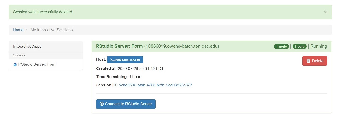
Rstudio will open up in a new tab with a custom and isolated environment that is set through a container-based solution. This will create a folder under $HOME/osc_classes/course_ID for each user. Please note that inside the Rstudio, you won't be able to access any files other than class materials. However, you can access the class directory outside of Rstudio to upload or download files.

You can quit a Rstudio session by clicking on File from the top tabs then on the Quit. This will only quit the session, but the resource you requested is still held until walltime limit is reached. To release the resource, please click on DELETE in the Rstudio launch page.
Shared Access
PI can store and share materials like data, scripts, etc, and R packages with the class. We will set up a project space for the project ID of the course. This project space will be created under /fs/ess/project_ID.
Shared R packages
Once the class module is ready, PI can access the course at class.osc.edu under the Rstudio job submission page. PI can launch the course environment and install R packages for the class.
It is important to install R packages for the class only in the class R environment after launching the Rstudio interface for the course. If you install R packages without launching class Rstudio, R will have access to your personnel R libraries at $HOME and could affect the installation process.
After launching Rstudio, please run the .libPaths() as follows
> .libPaths()
[1] "/users/PZS0711/akachlan/osc_classes/OSCWORKSHOP/R"
[2] "/fs/ess/PZS1117/OSCWORKSHOP/Rpkgs"
[3] "/apps/R/gnu/9.1/4.0.2/site/pkgs"
[4] "/apps/R/gnu/9.1/4.0.2/lib64/R/library"
Here you will see four R library paths. The last two are system R library paths and are accessible for all OSC users. OSC installs a number of popular R packages at the site location. You can check available packages with library() command. The first path is a personal R library of each user in the course environment and is not shared with students. The second lib path is accessible to all students of the course(Eg: /fs/ess/PZS0687/OSCWORKSHOP/Rpkgs). PI should install R packages in this library to share with the class. As a precaution, it is a good idea to eliminate PI's personal R library from .libPaths() before R package installation as follows. Please note that this step is needed to be done only when preparing course materials by PI.
> .libPaths(.libPaths()[-1])
> .libPaths()
[1] "/fs/ess/PZS1117/OSCWORKSHOP/Rpkgs"     "/apps/R/gnu/9.1/4.0.2/site/pkgs"
[3] "/apps/R/gnu/9.1/4.0.2/lib64/R/library"
Now there is only one writable R library path such that all packages will be installed into this library path and shared for all users.
PI can install all packages required for the class using install.packages() function. Once the installation is complete, students will have access to all those packages.
Please note that students can also install their own packages. Those packages will be installed into their personable library in the class environment i.e., the first path listed under .libPaths()
Shared materials
PI can share materials like data, scripts, and rmd files stored in /fs/ess/project_ID/course_ID/materials with students. When a student launch a Rstduio session, the directory will be copied to the student's workspace $HOME/osc_classes/courseID (destination). Please inform us if you want to use a source directory other than /fs/ess/project_ID/course_ID/materials. The student will see the directory materials on the landing page. PI can add files to the material source directory. New files will be copied to the destination every time using rsync when a new Rstudio session starts. But If PI modifies existing files, the changes won't be copied as the files were copied before. Therefore we recommend renaming the file after the update so that it will be copied.
Please limit the size of data stored in the material folders of your project space to a maximum of 3GB. Larger files can cause issues with the rsync process. If you have files that exceed this limit, we recommend hosting them outside the material folder within your project space. Students will still be able to access the data after launching RStudio. If you need assistance managing large files or have any other questions, please don't hesitate to reach out for support
There are several different ways to copy materials manually from a directory to students' workspace.
- On
class.osc.eduserver, click onFilesfrom the top tabs, then on$HOMEdirectory. From the top right, click onGo toand enter the storage path (Eg:/fs/ess/PZS1117/) in the box and press OK. This will open up storage path and users can copy files. Open the class folder from the$HOMEtree shown on left and paste files there. All files copied to$HOME/osc_classes/course_IDwill appear in the Rstudio FIle browser.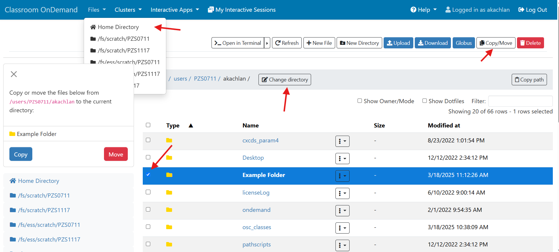
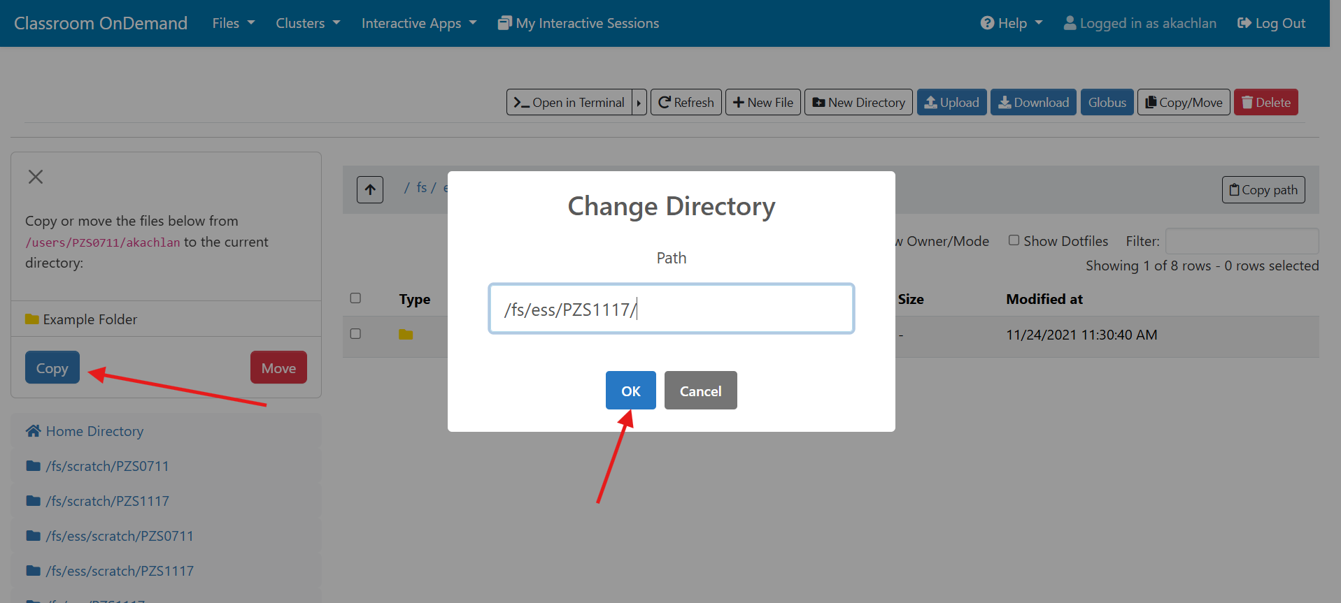
- On
class.osc.eduserver, Click onClustersfrom the top tabs, then onAscend Shell Access. This will open up a terminal on Ascend where students can enter Unix command for copying. Eg:
cp -r /fs/ess/PZS1117/OSCWORKSHOP/materials $HOME/osc_classes/course_ID
Please note that$HOME/osc_classes/course_IDwill be created only after launching Rstudio instance at least once. - Students can also upload material directly to Rstudio using the
uploadtab located in theFile browserof Rstudio from their local computer. This assumes they have already downloaded materials to their computers.

Checklist for PIs
- Apply for a classroom project ID that is unique to the course
- Add yourself, PI, to the project as an authorized user.
- Inform us about additional requirements such as R version or other software
- Once the class module is ready, create class materials under the storage path, and install R packages in the class environment.
- Invite students to the project at my.osc.edu to give them access to the project ID.
Please reach out to oschelp@osc.edu if you have any questions.
Using nbgrader for Classroom
Using ngbrader in Jupyter
Install nbgrader
You can install nbgrader in a notebook:
- Launch a Juypter session from class.osc.edu
- Open a new notebook
- To Install nbgrader, run:
!pip install nbgrader
!jupyter nbextension install --sys-prefix --py nbgrader --overwrite
!jupyter nbextension enable --sys-prefix --py nbgrader
!jupyter serverextension enable --sys-prefix --py nbgrader
To check the installed extensions, run
!jupyter nbextension list
There are six enabled extensions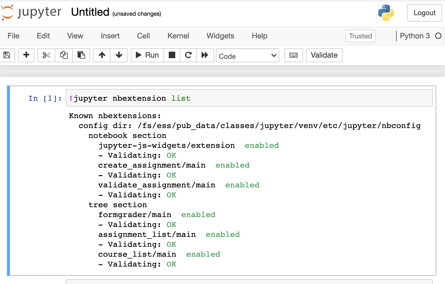
Configure nbgrader
In order to upload and collect assignments, nbgrader requires a exchange directory with write permissions for everyone. For example, to create a directory in project space, run:
%%bash
mkdir -p /fs/ess/projectID/courseID/exchange
chmod a+wx /fs/ess/projectID/courseID/exchange
Then get your cousre ID for configuratin. In a notebook, run:
%%bash
echo $OSC_CLASS_ID
Finally create the nbgrader configuration at the root of the workspace. In a notebook, run
%%file nbgrader_config.py
c = get_config()
c.CourseDirectory.course_id = "courseID"     # it must be the value of $OSC_CLASS_ID
c.Exchange.root = "/fs/ess/projectID/courseID/exchange"
c.Exchange.timezone = 'EST'
Once the file is created, you can launch a new Jupyter session then start creating assignments. For using nbgrader, please refer the nbgrader documents.
Access assignments
To let students access the assignments, students need to have the following configuration file in the root of their workspace:
%%file nbgrader_config.py
c = get_config()
c.Exchange.root = "/fs/ess/projectID/courseID/exchange"
HOWTO
Our HOWTO collection contains short tutorials that help you step through some of the common (but potentially confusing) tasks users may need to accomplish, that do not quite rise to the level of requiring more structured training materials. Items here may explain a procedure to follow, or present a "best practices" formula that we think may be helpful.
Service:
Using Software on Pitzer RHEL 7
While OSC has upgraded the Pitzer cluster to RHEL 9, you may encounter difficulties when migrating jobs from RHEL 7 to the new system. To help you continue your research, we provide a containerized RHEL 7 environment on Pitzer RHEL 9. This container replicates the original RHEL 7 system and software environment used on Pitzer.
Note: This containerized RHEL7 environment is a temporary solution and may be terminated at any time without prior notice.
Note: If you need to compile software with Intel compilers version 19 or earlier, which require a license, please contact oschelp@osc.edu to request access to the license.
Reusing Job Scripts
Assume you have an existing job script that previously worked on Pitzer RHEL 7 (e.g., my_rhel7_job.sh):
#!/bin/bash
#SBATCH --nodes=1
#SBATCH --ntasks-per-node=4

my_rhel7_program
To run this script within the RHEL 7 container on Pitzer RHEL 9, prepare a new job script that uses the container wrapper, such as my_rhel7_job_in_container.sh:
#!/bin/bash
#SBATCH --nodes=1
#SBATCH --ntasks-per-node=4

/apps/share/tools/rhel7_wrapper.sh ./my_rhel7_job.sh
Then submit the job after making my_rhel7_job.sh an executable
chmod +x my_rhel7_job.sh
sbatch my_rhel7_job_in_container.sh
Running a MPI program
We have disabled Slurm support inside the container due to certain technical issues. Therefore, any Slurm-specific commands in your job script (such as srun or sbcast) will not work. You should replace them with alternatives such as mpirun/mpiexec and cp, respectively.
Please note that MVAPICH2 is built only with Slurm support, so there is no native mpirun/mpiexec command available for it inside the container. Instead, you can use Intel-MPI or OpenMPI, which provide their own mpiexec commands.
Below are example replacements for srun:
# OpenMPI
mpiexec --bind-to none <your_program>

# Intel-MPI
mpiexec -launcher ssh <your_program>
Note: Multi-node MPI jobs are not supported in this containerized environment.
GPU support and extra bind path
If your job requires GPUs, append the --nv option:
/apps/share/tools/rhel7_wrapper.sh --nv ./my_rhel7_job.sh
By default, you can access your own home directory. If you need access to another user's home directory that has been shared with you, use the --bind option:
/apps/share/tools/rhel7_wrapper.sh --bind /someone/else/home ./my_rhel7_job.sh
Working Interactively in the RHEL 7 Environment
In some cases, you may need to recompile your program within the RHEL 7 environment. You can either use the job script mentioned above or launch an interactive container shell session after starting an interactive job:
/apps/share/tools/rhel7_shell.sh
Once inside the container shell, initialize the RHEL 7 environment by running:
source /etc/profile.d/lmod.sh
source /etc/profile.d/z00_StdEnv.sh
module rm xalt
Or, as a shortcut:
. /apps/share/tools/init_rhel7.sh
You can verify that the RHEL 7 environment is properly set up by running:
module list
The options --nv and --bind are also available in the rhel7_shell.sh script.
Supercomputer:
Fields of Science:
HOW TO: Look at requested time accuracy using XDMoD
The XDMoD tool at xdmod.osc.edu can be used to get an overview of how accurate the requested time of jobs are with the elapsed time of jobs.
To request an amount of time for a job, you can use the following header.
#SBATCH --time=xx:xx:xx
The elapsed time is how long the job ran for before completing. This can be obtained for completed jobs using the sacct command.
$ sacct -u <username> --format=jobid,account,elapsed
It is important to understand that the requested time is used when scheduling a submitted job. A longer requested time will also increase the wait time, as it will take longer to reserve the requested resources for that amount of time. This makes getting the requested job time as close to the expected elapsed time important for minimizing wait times.
The above method of checking elapsed time allows one to view the requested time accuracy for an individual job, but XDMoD can be used to do this for jobs submitted over a specified period of time.
First, login to xdmod.osc.edu. (See this page for more instructions.)
https://www.osc.edu/supercomputing/knowledge-base/xdmod_tool
Then, navigate to the Metric Explorer tab.
Look for the Metric Catalog on the left side of the page and expand the SUPREMM options. Select Wall Hours: Requested: Per Job and group by None.
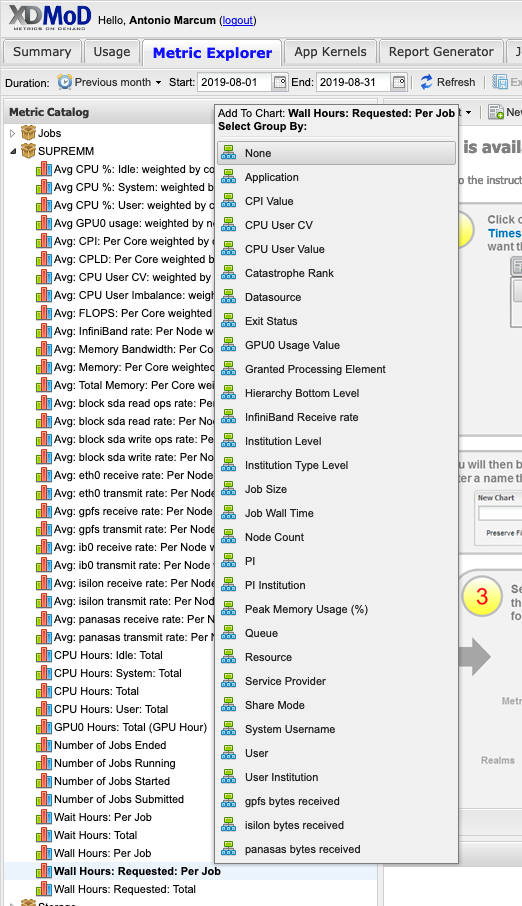
This will now show the average time requested.
The actual time data can be added by navigating to Add Data -> SUPREMM -> Wall Hours: Per Job.
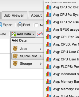

This will open a new window titled Data Series Definition, to change some parameters before showing the new data. In order to easily distinguish between elapsed and requested time, change the Display Type to Bar, then click add to view the new data.
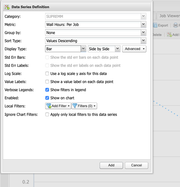
Now there is a line showing the average time requested by submitted jobs, and bars depicting the average time that elapsed to complete those jobs. Essentialy, the closer the bar is to the line, without intersecting the line, the more accurate the time predicition. If the bar intersects the line, then it may indicate the there was not enough time requested for a job to complete, but remember that these values are averages.

One can also view more detailed information about these jobs by clicking a data point and using the Show raw data option.
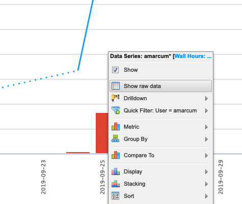
In order to have the Show raw data option, one may need to use the Drilldown option first to sort the jobs in that list by use or another metric.
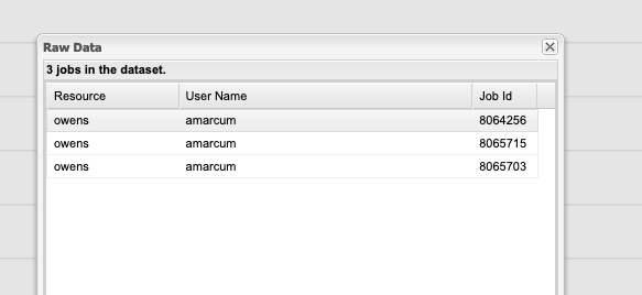
Service:
HOWTO: Add and Use DUO MFA
Options:
- Duo Mobile: You can install Duo Mobile on your smartphone or tablet. It will give you two ways to authenticate either through DUO push notification or DUO mobile passcode
- Text Message Passcode: You can register your phone and request a passcode via text message. It will send you a single use passcode via text message
- Phone Call: You can register your phone and request a phone call. It will call you and provide a single use passcode
- Security keys: You can purchase security keys such as a YubiKey to access web applications.
- If you need for SSH connection, please purchase YubiKeys that support "OATH - HOTP" and email OSC Help to schedule a meeting and get your security key enrolled in OSC's Duo instance. See this Use YubiKeys with Duo page for additional information.
HOWTO: Collect performance data for your program
This page outlines ways to generate and view performance data for your program using tools available at OSC.
Intel Tools
This section describes how to use performance tools from Intel. Make sure that you have an Intel module loaded to use these tools.
Intel VTune
Intel VTune is a tool to generate profile data for your application. Generating profile data with Intel VTune typically involves three steps:
1. Prepare the executable for profiling.
You need executables with debugging information to view source code line detail: re-compile your code with a -g option added among the other appropriate compiler options. For example:
mpicc wave.c -o wave -g -O3
2. Run your code to produce the profile data.
Profiles are normally generated in a batch job. To generate a VTune profile for an MPI program:
mpiexec <mpi args> amplxe-cl <vtune args> <program> <program args>
where <mpi args> represents arguments to be passed to mpiexec, <program> is the executable to be run, <vtune args> represents arguments to be passed to the VTune executable amplxe-cl, and <program args> represents arguments passed to your program.
For example, if you normally run your program with mpiexec -n 12 wave_c, you would use
mpiexec -n 12 amplxe-cl -collect hotspots -result-dir r001hs wave_c
To profile a non-MPI program:
amplxe-cl <vtune args> <program> <program args>
The profile data is saved in a .map file in your current directory.
As a result of this step, a subdirectory that contains the profile data files is created in your current directory. The subdirectory name is based on the -result-dir argument and the node id, for example, r001hs.o0674.ten.osc.edu.
3. Analyze your profile data.
You can open the profile data using the VTune GUI in interactive mode. For example:
amplxe-gui r001hs.o0674.ten.osc.edu
One should use an OnDemand VDI (Virtual Desktop Interface) or have X11 forwarding enabled (see Setting up X Windows). Note that X11 forwarding can be distractingly slow for interactive applications.
Intel APS
Intel's Application Performance Snapshot (APS) is a tool that provides a summary of your application's performance . Profiling HPC software with Intel APS typically involves four steps:
1. Prepare the executable for profiling.
Regular executables can be profiled with Intel APS. but source code line detail will not be available. You need executables with debugging information to view source code line detail: re-compile your code with a -g option added among the other approriate compiler options. For example:
mpicc wave.c -o wave -tcollect -O3
2. Run your code to produce the profile data directory.
Profiles are normally generated in a batch job. To generate profile data for an MPI program:
mpiexec -trace <mpi args> <program> <program args>
where <mpi args> represents arguments to be passed to mpiexec, <program> is the executable to be run and <program args> represents arguments passed to your program.
For example, if you normally run your program with mpiexec -n 12 wave_c, you would use
mpiexec -n 12 wave_c
To profile a non-MPI program:
aps <program> <program args>
The profile data is saved in a subdirectory in your current directory. The directory name is based on the date and time, for example, aps_result_YYYYMMDD/.
3. Generate the profile file from the directory.
To generate the html profile file from the result subdirectory:
aps --report=./aps_result_YYYYMMDD
to create the file aps_report_YYYYMMDD_HHMMSS.html.
4. Analyze the profile data file.
You can open the profile data file using a web browswer on your local desktop computer. This option typically offers the best performance.
Linaro Tools
This section describes how to use performance tools from ARM.
Linaro MAP
Instructions for how to use MAP is available here.
Linaro DDT
Instructions for how to use DDT is available here.
Linaro Performance Reports
Instructions for how to use Performance Reports is available here.
Other Tools
This section describes how to use other performance tools.
HPC Toolkit
Rice University's HPC Toolkit is a collection of performance tools. Instructions for how to use it at OSC is available here.
TAU Commander
TAU Commander is a user interface for University of Oregon's TAU Performance System. Instructions for how to use it at OSC is available here.
Service:
HOWTO: Create and Manage Python Environments
While our Python installations come with many popular packages installed, you may come upon a case in which you need an additional package that is not installed. If the specific package you are looking for is available from anaconda.org (formerly binstar.org), you can easily install it and required dependencies by using the conda package manager.
Procedure
The following steps are an example of how to set up a Python environment and install packages to a local directory using conda. We use the name local for the environment, but you may use any other name.
Load proper Python module
We have python and Miniconda3 modules. python and miniconda3 module is based on Conda package manager. python modules are typically recommended when you use Python in a standard environment that we provide. However, if you want to create your own python environment, we recommend using miniconda3 module, since you can start with minimal configurations.
module load miniconda3/24.1.2-py310
Configure Conda (first time use)
The first time you use conda, it is recommend to configure it to use the desired channels and options. A number of channels exist with different packages and licensing requirements. While academic users are generally unrestricted, commercial users may be subject to terms of service requiring license purchasing. Commercial users are encouraged to check with their organization regarding licensing. Please see Anaconda, Inc. Terms of Service for details.
To avoid using proprietary packages from the defaults channel, users can remove it:
conda config --remove channels defaults
and add the alternative conda-forge channel instead:
conda config --add channels conda-forge
OSC recommends setting strict channel priority:
conda config --set channel_priority strict
If strict channel priority makes required dependencies unavailable, it can be disabled:
conda config --set channel_priority flexible
Create Python installation to local directory
Three alternative create commands are listed. These cover the most common cases.
CREATE NEW ENVIRONMENT
The following will create a minimal Python installation without any extraneous packages:
conda create -n local
CLONE BASE ENVIRONMENT
If you want to clone the full base Python environment from the system, you may use the following create command:
conda create -n local --clone base
CREATE NEW ENVIRONMENT WITH SPECIFIC PACKAGES
You can augment the command above by listing specific packages you would like installed into the environment. For example, the following will create a minimal Python installation with only the specified packages (in this case, numpy and babel):
conda create -n local numpy babel
By default, conda will install the newest versions of the packages it can find. Specific versions can be specified by adding =<version> after the package name. For example, the following will create a Python installation with Python version 2.7 and NumPy version 1.16:
conda create -n local python=2.7 numpy=1.16
CREATE NEW ENVIRONMENT WITH A SPECIFIC location
By default, conda will create the environment in your home location $HOME. To specify a location where the local environment is created, for example, in the project space /fs/ess/ProjectID, you can use the following command:
conda create --prefix /fs/ess/ProjectID/local
To activate the environment, use the command:
source activate /fs/ess/ProjectID/local
To verify that a clone has been created, use the command
conda info -e
For additional conda command documentation see https://docs.conda.io/projects/conda/en/latest/commands.html#conda-general-commands
Activate environment
Before the created environment can be used, it must be activated.
For the bash shell:
source activate local
At the end of the conda create step, you may saw a message from the installer that you can use conda activate command for activating environment. But, please don't use conda activate command, because it will try to update your shell configuration file and it may cause other issues. So, please use source activate command as we suggest above.
If you've previously utilized
conda init to enable the conda activate command, your shell configuration file such as .bashrc would have been altered with conda-specific lines. Upon activation of your environment using source activate, you may notice that the source activate/deactivate commands cease to function. However, we will be updating miniconda3 modules by May 15th 2024 to ensure that conda activate no longer alters the .bashrc file. Consequently, you can safely remove the conda-related lines between # >>> conda initialize >>> and # <<< conda initialize <<< from your .bashrc file and continue using the conda activate command.On newer versions of Anaconda on the Pitzer cluster you may also need to perform the removal of the following packages before trying to install your specific packages:
conda remove conda-build
conda remove conda-env
Install packages
To install additional packages, use the conda install command. For example, to install the yt package:
conda install yt
By default, conda will install the newest version if the package that it can find. Specific versions can be specified by adding =<version> after the package name. For example, to install version 1.16 of the NumPy package:
conda install numpy=1.16
If you need to install packages with pip, then you can install pip in your virtual environment by
conda install pip
Then, you can install packages with pip as
pip install PACKAGE
Please make sure that you have installed pip in your environment not using one from the miniconda module. The pip from the miniconda module will give access to the packages from the module to your environment which may or may not be desired. Also set export PYTHONNOUSERSITE=True to prevent packages from user's .local path.
Test Python package
Now we will test our installed Python package by loading it in Python and checking its location to ensure we are using the correct version. For example, to test that NumPy is installed correctly, run
python -c "from __future__ import print_function; import numpy; print(numpy.__file__)"
and verify that the output generally matches
$HOME/.conda/envs/local/lib/python3.6/site-packages/numpy/__init__.py
To test installations of other packages, replace all instances of numpy with the name of the package you installed.
Remember, you will need to load the proper version of Python before you go to use your newly installed package. Packages are only installed to one version of Python.
Install your own Python packages
If the method using conda above is not working, or if you prefer, you can consider installing Python packages from the source. Please read HOWTO: install your own Python packages.
But I use virtualenv and/or pip!
See the comparison to these package management tools here:
https://docs.conda.io/projects/conda/en/latest/commands.html#conda-vs-pip-vs-virtualenv-commands
Use pip only without conda package manager
pip installations are supported:
module load python
module list                            # check which python you just loaded
pip install --user --upgrade PACKAGE   # where PACKAGE is a valid package name
Note the default installation prefix is set to the system path where OSC users cannot install the package. With the option --user, the prefix is set to $HOME/.local where lib, bin, and other top-level folders for the installed packages are placed. Finally, the option --upgrade will upgrade the existing packages to the newest available version.
The one issue with this approach is portability with multiple Python modules. If you plan to stick with a single Python module, then this should not be an issue. However, if you commonly switch between different Python versions, then be aware of the potential trouble in using the same installation location for all Python versions.
Use pip in a Python virtual environment (Python 3 only)
Typically, you can install packages with the methods shown in Install packages section above, but in some cases where the conda package installations have no source from conda channels or have dependency issues, you may consider using pip in an isolated Python virtual environment.
To create an isolated virtual environment:
module reset
python3 -m venv --without-pip $HOME/venv/mytest --prompt "local"
source $HOME/venv/mytest/bin/activate
(local) curl https://bootstrap.pypa.io/get-pip.py |python     # get the newest version of pip
(local) deactivate
where we use the path $HOME/venv/mytest and the name local for the environment, but you may use any other path and name.
To activate and deactivate the virtual environment:
source $HOME/venv/mytest/bin/activate
(local) deactivate
To install packages:
source $HOME/venv/mytest/bin/activate
(local) pip install PACKAGE
You don't need the --user option within the virtual environment.
Use uv for virtual environments and package management
uv is a fast Python package and virtual environment manager developed by Astral. It provides functionality provided by both venv and pip, but is significantly faster at dependency resolution. Some users who do not need Conda packages or cross-language support in their project may prefer to use uv for its speed.
To learn more about using uv, see HOWTO: Use uv for Python at OSC.
Further Reading
Conda Test Drive: https://conda.io/docs/test-drive.html
HOWTO: Install Tensorflow locally
This documentation describes how to install tensorflow package locally in your $HOME space. For more details on Tensorflow see the software page.
Load python module
module load miniconda3/24.1.2-py310
We already provide some versions of tensorflow centrally installed on our clusters. To see the available versions, run conda list tensorflow. See software page for software details and usage instructions on the clusters.
If you need to install tensorflow versions not already provided or would like to use tensorflow in a conda environment proceed with the tutorial below.
Create Python Environment
First we will create a conda environment which we will later install tensorflow into. See HOWTO: Create and Manage Python Environments for details on how to create and setup your environemnt.
Make sure you activate your environment before proceeding:
source activate MY_ENV
Install package
Install the latest version of tensorflow.
conda install tensorflow
You can see all available version for download on conda with conda search tensorflow
There is also a gpu compatable version called tensorflow-gpu
If there are errors on this step you will need to resolve them before continuing.
Test python package
Now we will test tensorflow package by loading it in python and checking its location to ensure we are using the correct version.
python -c "import tensorflow;print (tensorflow.__file__)"
Output:
$HOME/.conda/envs/MY_ENV/lib/python3.9/site-packages/tensorflow/__init__.py
Remember, you will need to load the proper version of python before you go to use your newly installed package. Packages are only installed to one version of python.
Please refer HOWTO: Use GPU with Tensorflow and PyTorch if you would like to use tenorflow with Gpus.
HOWTO: Install Python packages from source
While we provide a number of Python packages, you may need a package we do not provide. If it is a commonly used package or one that is particularly difficult to compile, you can contact OSC Help for assistance. We also have provided an example below showing how to build and install your own Python packages and make them available inside of Python. These instructions use "bash" shell syntax, which is our default shell. If you are using something else (csh, tcsh, etc), some of the syntax may be different.
Please consider using conda Python package manager before you try to build Python using the method explained here. We have instructions on conda here.
Note: any custom packages you install in your environment (not installed from repos) will not be tracked by conda/pip. Therefore, actions like cloning your environment will not copy over the custom packages and you will need to install again for each new conda environment.
Gather your materials
First, you need to collect what you need in order to perform the installation. We will do all of our work in $HOME/local/src. You should make this directory now.
mkdir -p $HOME/local/src
Next, we will need to download the source code for the package we want to install. In our example, we will use NumExpr. (NumExpr is already available through conda, so it is recommended you use conda to install it: tutorial here. The following steps are simply an example of the procedure you would follow to perform an installation of software unavailable in conda or pip). You can either download the file to your desktop and then upload it to OSC, or directly download it using the wget utility (if you know the URL for the file).
cd ~/local/src
wget https://github.com/pydata/numexpr/releases/download/v2.8.4/numexpr-2.8.4.tar.gz
Next, extract the downloaded file. In this case, since it's a "tar.gz" format, we can use tar to decompress and extract the contents.
tar xvfz numexpr-2.8.4.tar.gz
You can delete the downloaded archive now or keep it should you want to start the installation from scratch.
Build it!
Environment
To build the package, we will want to first create a temporary environment variable to aid in installation. We'll call INSTALL_DIR.
export INSTALL_DIR=${HOME}/local/numexpr/2.8.4
We are roughly following the convention we use at the system level. This allows us to easily install new versions of software without risking breaking anything that uses older versions. We have specified a folder for the program (numexpr), and for the version (2.8.4). To be consistent with Python installations, we will create a second temporary environment variable that will contain the actual installation location.
export TREE=${INSTALL_DIR}/lib/python3.6/site-packages
Next, make the directory tree.
mkdir -p $TREE
Compile
To compile the package, we should switch to the GNU compilers. The system installation of Python was compiled with the GNU compilers, and this will help avoid any unnecessary complications. We will also load the Python package, if it hasn't already been loaded.
module swap intel gnu
module load python/3.6-conda5.2
Next, build it. This step may vary a bit, depending on the package you are compiling. You can execute python setup.py --help to see what options are available. Since we are overriding the install path to one that we can write to and that fits our management plan, we need to use the --prefix option.
NumExpr build also requires us to set the PYTHONPATH variable before building:
export PYTHONPATH=$PYTHONPATH:~/local/numexpr/2.8.4/lib/python3.6/site-packages
Find the setup.py file:
cd numexpr-2.8.4
Now to build:
python setup.py install --prefix=$INSTALL_DIR
Make it usable
At this point, the package is compiled and installed in ~/local/numexpr/2.8.4/lib/python3.6/site-packages. Occasionally, some files will be installed in ~/local/numexpr/2.8.4/bin as well. To ensure Python can locate these files, we need to modify our environment.
Manual
The most immediate way -- but the one that must be repeated every time you wish to use the package -- is to manually modify your environment. If files are installed in the "bin" directory, you'll need to add it to your path. As before, these examples are for bash, and may have to be modified for other shells. Also, you will have to modify the directories to match your install location.
export PATH=$PATH:~/local/numexpr/2.8.4/bin
And for the Python libraries:
export PYTHONPATH=$PYTHONPATH:~/local/numexpr/2.8.4/lib/python3.6/site-packages
Hardcode it
We don't recommend this option, as it is less flexible and can cause conflicts with system software. But if you want, you can modify your .bashrc (or similar file, depending on your shell) to set these environment variables automatically. Be extra careful; making a mistake in .bashrc (or similar) can destroy your login environment in a way that will require a system administrator to fix. To do this, you can copy the lines above modifying $PATH and $PYTHONPATH into .bashrc. Remember to test them interactively first. If you destroy your shell interactively, the fix is as simple as logging out and then logging back in. If you break your login environment, you'll have to get our help to fix it.
Make a module (recommended!)
This is the most complicated option, but it is also the most flexible, as you can have multiple versions of this particular software installed and specify at run-time which one to use. This is incredibly useful if a major feature changes that would break old code, for example. You can see our tutorial on writing modules here, but the important variables to modify are, again, $PATH and $PYTHONPATH. You should specify the complete path to your home directory here and not rely on any shortcuts like ~ or $HOME. Below is a modulefile written in Lua:
If you are following the tutorial on writing modules, you will want to place this file in $HOME/local/share/lmodfiles/numexpr/2.8.4.lua:
-- This is a Lua modulefile, this file 2.8.4.lua can be located anywhere
-- But if you are following a local modulefile location convention, we place them in
-- $HOME/local/share/lmodfiles/
-- For numexpr we place it in $HOME/local/share/lmodfiles/numexpr/2.8.4.lua
-- This finds your home directory
local homedir = os.getenv("HOME")
prepend_path("PYTHONPATH",
pathJoin(homedir, "/local/numexpr/2.8.4/lib/python3.6/site-packages"))
prepend_path(homedir, "local/numexpr/2.8.4/bin")
Once your module is created (again, see the guide), you can use your Python package simply by loading the software module you created.
module use $HOME/local/share/lmodfiles/
module load numexpr/2.8.4
Service:
HOWTO: Use GPU with Tensorflow and PyTorch
GPU Usage on Tensorflow
Environment Setup
To begin, you need to first create and new conda environment or use an already existing one. See HOWTO: Create Python Environment for more details. In this example we are using miniconda3/24.1.2-py310 . You will need to make sure your python version within conda matches supported versions for tensorflow (supported versions listed on TensorFlow installation guide), in this example we will use python 3.9.
Once you have a conda environment created and activated we will now install tensorflow into the environment (In this example we will be using version 2.17.0 of tensorflow:
pip install tensorflow==2.17.0
Verify GPU accessability (Optional):
Now that we have the environment set up we can check if tensorflow can access the gpus.
To test the gpu access we will submit the following job onto a compute node with a gpu:
#!/bin/bash
#SBATCH --account <Project-Id>
#SBATCH --job-name Python_ExampleJob
#SBATCH --nodes=1
#SBATCH --time=00:10:00
#SBATCH --gpus-per-node=1


module load miniconda3/24.1.2-py310 cuda/12.3.0

source activate tensorflow_env


# run either of the following commands

python << EOF
import tensorflow as tf
print(tf.test.is_built_with_cuda())
EOF

python << EOF
from tensorflow.python.client import device_lib
print(device_lib.list_local_devices())
EOF
You will know tensorflow is able to successfully access the gpu if tf.test.is_built_with_cuda() returns True and device_lib.list_local_devices() returns an object with /device:GPU:0 as a listed device.
At this point tensorflow-gpu should be setup to utilize a GPU for its computations.
GPU vs CPU
A GPU can provide signifcant performace imporvements to many machine learnings models. Here is an example python script demonstrating the performace improvements. This is ran on the same environment created in the above section.
from timeit import default_timer as timer
import tensorflow as tf
from tensorflow import keras
import numpy as np


(X_train, y_train), (X_test, y_test) = keras.datasets.cifar10.load_data()


# scaling image values between 0-1
X_train_scaled = X_train/255
X_test_scaled = X_test/255

# one hot encoding labels
y_train_encoded = keras.utils.to_categorical(y_train, num_classes = 10)
y_test_encoded = keras.utils.to_categorical(y_test, num_classes = 10)

def get_model():
    model = keras.Sequential([
        keras.layers.Flatten(input_shape=(32,32,3)),
        keras.layers.Dense(3000, activation='relu'),
        keras.layers.Dense(1000, activation='relu'),
        keras.layers.Dense(10, activation='sigmoid')
    ])

    model.compile(optimizer='SGD',
              loss='categorical_crossentropy',
              metrics=['accuracy'])
    return model

# GPU
with tf.device('/GPU:0'):
    start = timer()
    model_cpu = get_model()
    model_cpu.fit(X_train_scaled, y_train_encoded, epochs = 1)
    end = timer()


print("GPU time: ", end - start)

# CPU
with tf.device('/CPU:0'):
    start = timer()
    model_gpu = get_model()
    model_gpu.fit(X_train_scaled, y_train_encoded, epochs = 1)
    end = timer()

print("CPU time: ", end - start)
Example code sampled from here
The above code was then submitted in a job with the following script:
#!/bin/bash
#SBATCH --account <Project-Id>
#SBATCH --job-name Python_ExampleJob
#SBATCH --nodes=1
#SBATCH --time=00:10:00
#SBATCH --gpus-per-node=1

module load miniconda3/24.1.2-py310 cuda/12.3.0

source activate tensorflow_env

python tensorflow_example.py
Make sure you request a gpu! For more information see GPU Computing
As we can see from the output, the GPU provided a signifcant performace improvement.
GPU time:  3.7491355929996644

CPU time:  78.8043485119997
Usage on Jupyter
If you would like to use a gpu for your tensorflow project in a jupyter notebook follow the below commands to set up your environment.
To begin, you need to first create and new conda environment or use an already existing one. See HOWTO: Create Python Environment for more details. In this example we are using python/3.6-conda5.2
Once you have a conda environment created and activated we will now install tensorflow-gpu into the environment (In this example we will be using version 2.4.1 of tensorflow-gpu:
conda install tensorflow-gpu=2.4.1
Now we will setup a jupyter kernel. See HOWTO: Use a Conda/Virtual Environment With Jupyter for details on how to create a jupyter kernel with your conda environment.
Once you have the kernel created see Usage section of Python page for more details on accessing the Jupyter app from OnDemand.
When configuring your notebook make sure to select a GPU enabled node and a cuda version.
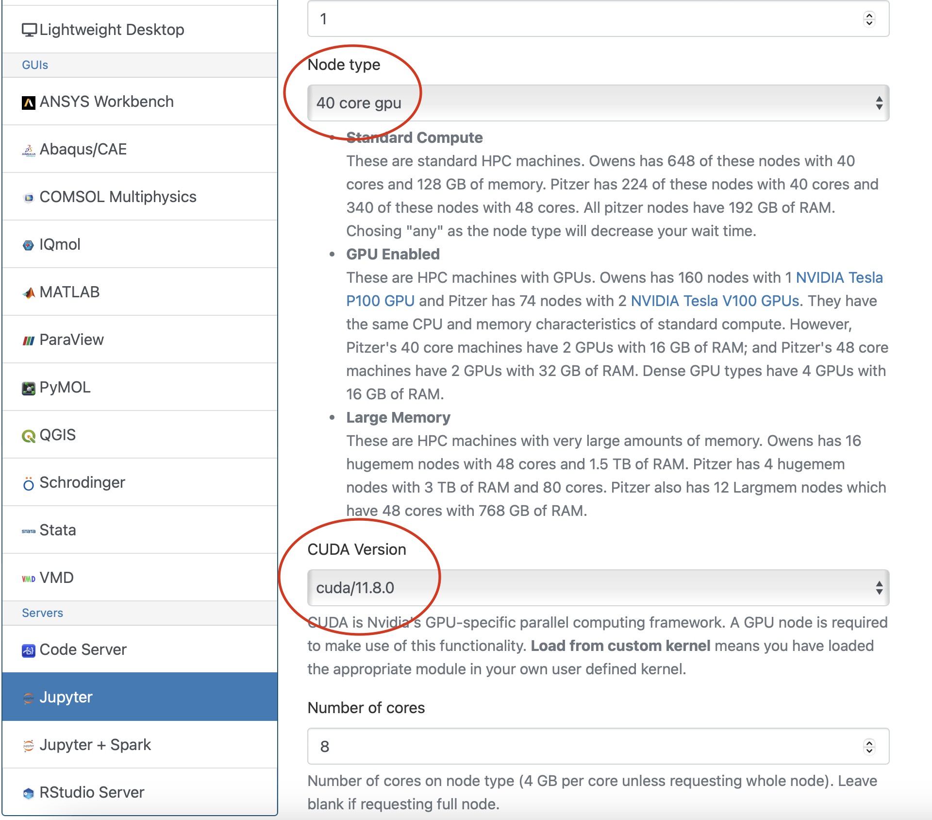
Now you are all setup to use a gpu with tensorflow on a juptyer notebook.
GPU Usage on PyTorch
Environment Setup
To begin, you need to first create and new conda environment or use an already existing one. See HOWTO: Create Python Environment for more details. In this example we are using miniconda3/24.1.2-py310
Once you have a conda environment created and activated we will now install pytorch into the environment (In the example we will be using version 2.3.0 of pytorch:
conda install pytorch=2.3.0
Verify GPU accessability (Optional):
Now that we have the environment set up we can check if pytorch can access the gpus.
To test the gpu access we will submit the following job onto a compute node with a gpu:
#!/bin/bash
#SBATCH --account <Project-Id>
#SBATCH --job-name Python_ExampleJob
#SBATCH --nodes=1
#SBATCH --time=00:10:00
#SBATCH --gpus-per-node=1


module load miniconda3/24.1.2-py310 cuda/12.3.0

source activate pytorch_env


python << EOF
import torch
print(torch.cuda.is_available())
device = torch.device("cuda:0" if torch.cuda.is_available() else "cpu")
print(device)
EOF
You will know pytorch is able to successfully access the gpu if torch.cuda.is_available() returns True and torch.device("cuda:0" if torch.cuda.is_available() else "cpu") returns cuda:0 .
At this point PyTorch should be setup to utilize a GPU for its computations.
GPU vs CPU
Here is an example pytorch script demonstrating the performace improvements from GPUs
import torch
from timeit import default_timer as timer


# check for cuda availability
print("Cuda: ", torch.cuda.is_available())
device = torch.device("cuda:0" if torch.cuda.is_available() else "cpu")
print("Device: ", device)


#GPU
b = torch.ones(4000,4000).cuda() # Create matrix on GPU memory
start_time = timer()
for _ in range(1000):
    b += b
elapsed_time = timer() - start_time

print('GPU time = ',elapsed_time)


#CPU
a = torch.ones(4000,4000) # Create matrix on CPU memory
start_time = timer()
for _ in range(1000):
    a += a
elapsed_time = timer() - start_time

print('CPU time = ',elapsed_time)
The above code was then submitted in a job with the following script:
#!/bin/bash
#SBATCH --account <Project-Id>
#SBATCH --job-name Python_ExampleJob
#SBATCH --nodes=1
#SBATCH --time=00:10:00
#SBATCH --gpus-per-node=1

module load miniconda3/24.1.2-py310 cuda/12.3.0

source activate pytorch_env

python pytorch_example.py
Make sure you request a gpu! For more information see GPU Computing
As we can see from the output, the GPU provided a signifcant performace improvement.
GPU time =  0.0053490259997488465

CPU time =  4.232843188998231
Usage on Jupyter
If you would like to use a gpu for your PyTorch project in a jupyter notebook follow the below commands to set up your environment.
To begin, you need to first create and new conda environment or use an already existing one. See HOWTO: Create Python Environment for more details. In this example we are using miniconda3/24.1.2-py310
Once you have a conda environment created and activated we will now install pytorch into the environment (In the example we will be using version 2.3.0 of pytorch:
conda install pytorch=2.3.0
You also may need to install numba for PyTorch to access a gpu from the jupter notebook.
conda install numba=0.60.0
Now we will setup a jupyter kernel. See HOWTO: Use a Conda/Virtual Environment With Jupyter for details on how to create a jupyter kernel with your conda environment.
Once you have the kernel created see Usage section of Python page for more details on accessing the Jupyter app from OnDemand.
When configuring your notebook make sure to select a GPU enabled node and a cuda version.
Now you are all setup to use a gpu with PyTorch on a juptyer notebook.
Horovod
If you are using Tensorflow or PyTorch you may want to also consider using Horovod. Horovod will take single-GPU training scripts and scale it to train across many GPUs in parallel.
Supercomputer:
HOWTO: Use uv for Python at OSC
uv is a fast Python package and virtual environment manager developed by Astral. It provides functionality provided by both venv and pip, but is significantly faster at dependency resolution. Some users who do not need Conda packages or cross-language support in their project may prefer to use uv for its speed. Because uv is still under active development and its behavior may change between frequent releases, OSC does not currently provide it as a centrally managed software package. However, users who wish to use uv may install it in their home directory and manage their own installation.
Install uv
To install uv on OSC systems, please manually download the install.sh script for the latest release:
wget https://astral.sh/uv/install.sh
Then, run the following commands to install uv in its own folder in your home directory:
chmod +x install.sh

mkdir -p $HOME/osc_apps/uv

UV_INSTALL_DIR="$HOME/osc_apps/uv" INSTALLER_NO_MODIFY_PATH=1 ./install.sh
The default uv installation procedure modifies a user's .bashrc and installs binaries into location that may not be appropriate for OSC systems. Installing uv into a dedicated location in your home directory as described above avoids creating conflicts with other modules.
Create a Local Module
After installation, OSC recommends you create a local module so that uv can be loaded into your PATH with module load uv/<version> when you want to use it. Modules allow you to dynamically alter your environment to define environment variables and bring executables, libraries, and other features into your shell's search paths. These instructions are for uv version 0.11.29.
We will be using the filename 0.11.29.lua ("version".lua). A simple Lua module for our uv installation would be:
-- Local Variables local name = "uv" local version = "0.11.29" -- Locate Home Directory local homedir = os.getenv("HOME") # This is for the path $HOME/osc_apps/uv local root = pathJoin(homedir, "osc_apps", name)-- Set Basic Paths prepend_path("PATH", pathJoin(root, "bin"))prepend_path("LD_LIBRARY_PATH", root .. "/lib") prepend_path("LIBRARY_PATH", root .. "/lib") prepend_path("INCLUDE", root .. "/include") prepend_path("CPATH", root .. "/include") prepend_path("PKG_CONFIG_PATH", root .. "/lib/pkgconfig")prepend_path("MANPATH", root .. "/share/man")
Copy this to a file and save it to your local module directory at $HOME/local/share/lmodfiles/uv.
Initializing Modules
To make this module usable, you need to tell lmod where to look for it. You can do this by issuing the command module use $HOME/osc_apps/lmodfiles in our example. You can see this change by performing module avail. This will allow you to load your software using module load uv/0.11.29.
More information about locally installing software and creating local modules can be found at HOWTO: Locally Installing Software.
Create a virtual environment
Before creating a virtual environment with uv, load your local uv module and an OSC Python module. If you do not load a Python module, uv will install and manage its own version of Python, which may be less optimized for OSC's systems.
To load these modules:
module load python/<version> uv/<version>
You can use module spider python to see which versions of python are available on a given system.
Then, to create a uv virtual environment, run:
uv venv --no-managed-python local
This creates an environment in the current directory called local. Using --no-managed-python means that uv will use the current Python module that you have loaded.
Activate and deactivate the virtual environment
First, load the Python module you used when you created the enviroment:
module load python/<version>
To activate your uv virtual environment (named local here), run:
source local/bin/activate
To deactivate your uv virtual environment, run:
deactivate
Install packages
uv can install packages from PyPi. To install a package with uv, run:
uv pip install package
Where package is the name of the package you want to install.
Further Reading
HOWTO: Debugging Tips
This article focuses on debugging strategies for C/C++ codes, but many are applicable to other languages as well.
Rubber Duck Debugging
This approach is a great starting point. Say you have written some code, and it does not do what you expect it to do. You have stared at it for a few minutes, but you cannot seem to spot the problem.
Try explaining what the problem is to a rubber duck. Then, walk the rubber duck through your code, line by line, telling it what it does. Don’t have a rubber duck? Any inanimate object will do (or even an animate one if you can grab a friend).
It sounds silly, but rubber duck debugging helps you to get out of your head, and hopefully look at your code from a new perspective. Saying what your code does (or is supposed to do) out loud has a good chance of revealing where your understanding might not be as good as you think it is.
Printf() Debugging
You’ve written a whole bunch of new code. It takes some inputs, chugs along for a while, and then creates some outputs. Somewhere along this process, something goes wrong. You know this because the output is not at all what you expected. Unfortunately, you have no idea where things are going wrong in the code.
This might be a good time to try out printf() debugging. It’s as simple as its name implies: simply add (more) printf() statements to your code. You’ve likely seen this being used. It’s the name given to the infamous ‘printf(“here”);’ calls used to verify that a particular codepath is indeed taken.
Consider printing out arguments and return values to key functions. Or, the results or summary statistics from large calculations. These values can be used as “sanity checks” to ensure that up until that point in the code, everything is going as expected.
Assertion calls, such as "assert(...)", can also be used for a similar purpose. However, often the positive feedback you get from print statements is helpful in when you’re debugging. Seeing a valid result printed in standard out or a log file tells you positively that at least something is working correctly.
Debuggers
Debuggers are tools that can be used to interactively (or with scripts) debug your code. A fairly common debugger for C and C++ codes is gdb. Many guides exist online for using gdb with your code.
OSC systems also provide the ARM DDT debugger. This debugger is designed for use with HPC codes and is arguably easier to use than gdb. It can be used to debug MPI programs as well.
Debuggers allow you to interact with the program while it is running. You can do things like read and write variable values, or check to see if/when certain functions are called.
Testing
Okay, this one isn’t exactly a debugging strategy. It’s a method to catch bugs early, and even prevent the addition of bugs. Writing a test suite for your code that’s easy to run (and ideally fast) lets you test new changes to ensure they don’t break existing functionality.
There are lots of different philosophies on testing software. Too many to cover here. Here’s two concepts that are worth looking into: unit testing and system testing.
The idea behind unit testing is writing tests for small “units” of code. These are often functions or classes. If you know that the small pieces that make up your code work, then you’ll have more confidence in the overall assembled program. There’s an added architecture benefit here too. Writing code that is testable in the first place often results in code that’s broken up into separate logical pieces (google “separation of concerns”). This makes your code more modular and less “spaghetti-like”. Your code will be easier to modify and understand.
The second concept – system testing – involves writing tests that run your entire program. These often take longer than unit tests, but have the added benefit that they’ll let you know whether or not your entire program still works after introducing a new change.
When writing tests (both system and unit tests), it’s often helpful to include a couple different inputs. Occasionally a program may work just fine for one input, but fail horribly with another input.
Minimal, Reproducible Example
Maybe your code takes a couple hours (or longer…) to run. There’s a bug in it, but every time you try to fix it, you have to wait a few hours to see if the fix worked. This is driving you crazy.
A possible approach to make your life easier is to try to make a Minimal, Reproducible Example (see this stackoverflow page for information).
Try to extract just the code that fails, from your program, and also its inputs. Wrap this up into a separate program. This allows you to run just the code that failed, hopefully greatly reducing the time it takes to test out fixes to the problem.
Once you have this example, can you make it smaller? Maybe take out some code that’s not needed to reproduce the bug, or shrink the input even further? Doing this might help you solve the problem.
Tools and other resources
- Compilers – compilers are your friends. Investigate the warning messages because these are likely candidates for unclear and buggy code. Chances are your compiler has a flag that can be used to enable more warnings than are on by default. GNU tools have “-Wall” and “-Wextra”. Modern compilers have extensive debugging options from memory analyzers to floating point arithmetic checkers. See the man page of your compiler.
- Valgrind is a tool that can be used for many types of debugging including looking for memory corruptions and leaks. However, it slows down your code a very sizeable amount. This might not be feasible for HPC codes
- ASAN (address sanitizer) is another tool that can be used for memory debugging. It is less featureful than Valgrind, but runs much quicker, and so will likely work with your HPC code.
- The Practice of Programming by Brian Kernighan and Rob Pike contains a very good chapter on debugging C and C++ programs.
- The Programming Pearls books by Jon Bentley contain good advice and examples of debugging. This includes a chapter where profiling identified a bug. See man gprof.
Service:
HOWTO: Establish durable SSH connections
In December 2021 OSC updated its firewall to enhance security. As a result, SSH sessions are being closed more quickly than they used to be. It is very easy to modify your SSH options in the client you use to connect to OSC to keep your connection open.
In ~/.ssh/config (use the command touch ~/.ssh/config to create it if there is no exisitng one), you can set 3 options:
TCPKeepAlive=no
ServerAliveInterval=60
ServerAliveCountMax=5
Please refer to your SSH client documentation for how to set these options in your client.
Service:
HOWTO: Estimating and Profiling GPU Memory Usage for Generative AI
Overview
Estimating GPU memory (VRAM) usage for training or running inference with large deep learning models is critical to both 1. requesting the appropriate resources for running your computation and 2. optimizing your job once it is setup. Out-of-memory (OOM) errors can be avoided by requesting appropriate resources and by better understanding memory usage during the job using memory profiling tools described here.
Estimating GPU Memory Usage for Inference
Estimated GPU VRAM in GB = 2x model parameters (in billions) + 1x context length (in thousands)
For example, for StableCode with 3 billion parameters and 16k context length, we estimate 6GB for model weights + 16GB for overhead, totaling 22 GB estimated to run inference. A model like this should fit on an A100 or H100 for inference.
This estimate assumes fp16 (half-precision). Quantization to lower precisions (8-bit, 4-bit, etc) will reduce memory requirements.
Estimating GPU Memory Usage for Training
Estimated GPU VRAM in GB = 40x model parameters (in billions)
For example, for LLaMA-3 with 7 billion parameters, we estimate minimum 280GB to train it. This exceeds the VRAM of even a single H100 accelerator, requiring distributed training. See HOWTO: PyTorch Fully Sharded Data Parallel (FSDP) for more details.
Of note, the training estimate assumes transformer-based architecture with Adam optimizer using mixed-precision (32bit and 16bit weights used) and is extrapolated from results here: Microsoft Deepspeed.
Activation checkpointing can reduce the memory demands, at the cost of increasing runtime.
Example GPU Memory Usage for Selected Models
| Model Name | Parameter count (billions) | Training / Inference | Batch Size | Context Length | min GPUs required | GPU Memory Usage (GB) |
|---|---|---|---|---|---|---|
| minGPT (GPT-2) | 0.12 | training | 216 | 1 V100 (16GB) | 9 | |
| T5 (small) | 3 | training | 4 | 1 H100 (94GB) | 81 | |
| T5 (medium) | 11 |
training |
4 | 8 H100s (94GB) | 760 | |
| Stable-Code-3b | 3 | inference (vllm) | 256 | 16k | 1 A100 (40GB) |
Model weights: 6GB Total usage: 7 (eager mode with 1k context length, 0.18 gpu), 10 (eager mode with 10k context length, 0.25 gpu), 14 (using 0.37 gpu), 20 (using 0.5 gpu), 36 (using 0.9 default gpu) |
| Falcon-7b-Instruct | 7 | inference (vllm) | 256 | 2k | 1 A100 (40GB) |
Model weights: 13GB Total usage: 15 (using 0.37 gpu), 20 (using 0.5 gpu), 36 (using 0.9 default) |
| CodeLlama-13b-Instruct-hf | 13 | inference (vllm) | 256 | 10k | 1 A100 (40GB) |
Model weights: 25GB |
| Gemma3:12b | 12 | inference (Ollama) | 512 | 2k | 1 V100 (16GB) | 11 |
Training memory usage was obtained from Prometheus data. Inference usage was measured with nvidia-smi and vllm or Ollama. Training usage generally follows the estimates above. Inference usage varies considerably depending on parameter size, context length and dtype precision. Vllm also uses a pre-allocation strategy which can increase estimated usage if left at its default 0.9. Eager mode vs CUDA graph mode trades memory footprint for speed.
Profiling GPU Memory Usage During Computation
There are a number of tools that can be used to gather more information about your job's GPU memory usage. Detailed memory usage can be helpful in debugging and optimizing your application to reduce memory footprint and increase performance.
GPU Usage script
The get_gpu_usage script is available on all OSC clusters. Start with this usage script to determine the maximum memory requirements of your job. Once your job has completed, provide the SLURM job ID (and optionally cluster name) to get the maximum memory usage on each GPU used on your job. For example,
$ get_gpu_usage -M cardinal 477503
Host c0813 GPU #0: 19834 MB
Host c0813 GPU #1: 33392 MB
Host c0813 GPU #2: 28260 MB
Host c0813 GPU #3: 28244 MB
Host c0823 GPU #0: 19808 MB
Host c0823 GPU #1: 33340 MB
Host c0823 GPU #2: 28260 MB
Host c0823 GPU #3: 28244 MB
Nvidia-smi Usage
nvidia-smi is a command-line tool available on all GPU-enabled compute nodes that lists processes and their GPU memory usage. Without any arguments, the output looks like the following:
[username@p0254 ~]$ nvidia-smi
Wed Nov 13 20:58:25 2024
+-----------------------------------------------------------------------------------------+
| NVIDIA-SMI 550.90.12              Driver Version: 550.90.12      CUDA Version: 12.4     |
|-----------------------------------------+------------------------+----------------------+
| GPU  Name                 Persistence-M | Bus-Id          Disp.A | Volatile Uncorr. ECC |
| Fan  Temp   Perf          Pwr:Usage/Cap |           Memory-Usage | GPU-Util  Compute M. |
|                                         |                        |               MIG M. |
|=========================================+========================+======================|
|   0  Tesla V100-PCIE-16GB           On  |   00000000:3B:00.0 Off |                  Off |
| N/A   27C    P0             37W /  250W |   13830MiB /  16384MiB |      0%      Default |
|                                         |                        |                  N/A |
+-----------------------------------------+------------------------+----------------------+

+-----------------------------------------------------------------------------------------+
| Processes:                                                                              |
|  GPU   GI   CI        PID   Type   Process name                              GPU Memory |
|        ID   ID                                                               Usage      |
|=========================================================================================|
|    0   N/A  N/A     27515      C   .../vllm_env/bin/python                     13818MiB |
+-----------------------------------------------------------------------------------------+
The example output above shows a V100 on a Pitzer compute node running a vllm inference server running a 3 billion parameter model and using about 14GB of GPU memory.
Summary statistics are available at the top, showing the GPUs available and their current and max memory available. Below, all running processes are shown, with the relevant GPU, PID, Process name, and GPU Memory Usage for that process.
The tool will show multiple GPU devices on the same node if more than one is available, but is limited to one node.
Additional arguments are available, as described in the official documentation.
To run nvidia-smi on the correct node, you will need to ssh to the node where your job is running. You can find the node hostname using the squeue command:
[username@pitzer-login02 ~]$ squeue -u username
             JOBID PARTITION     NAME     USER   ST       TIME  NODES NODELIST(REASON)
          32521417 gpudebug- interact   username  R       0:38      1 p0254
where "username" is your username. In the example above, "p0254" is the compute node you need to run the tool on. The jobid is also useful for other monitoring tools. See HOWTO: Monitoring and Managing Your Job for more details.
Grafana Dashboard Metrics
Grafana provides a dashboard that shows a timeline of GPU memory and usage over time during your job. The script job-dashboard-link.py
This can give you an idea of when in your job the memory usage peaked and how long it stayed there.
PyTorch memory snapshotting
This tool requires the following minor modifications to your code
- Start:
torch.cuda.memory._record_memory_history(max_entries=100000) - Save:
torch.cuda.memory._dump_snapshot(file_name) - Stop:
torch.cuda.memory._record_memory_history(enabled=None)
This creates a trace file that can viewed by using the javascript code available here. This trace contains information about which called memory allocations and deallocations. This information is sufficient in most cases to understand the memory behavior of your applications. The following two tools can be used to provide additional information, but are only recommended for advanced users.
See documentation here for more information on how to snapshot GPU memory usage while running PyTorch code.
PyTorch Profiler
"PyTorch Profiler is a tool that allows the collection of performance metrics during training and inference. Profiler’s context manager API can be used to better understand what model operators are the most expensive, examine their input shapes and stack traces, study device kernel activity and visualize the execution trace."
The PyTorch profiler also requires code modifications. It provides a suite of configuration options for what information to track and how to export it. The overhead (both in terms of slowing down your job and the size of the profile files) can get very large. There are multiple ways to view the profile data (tensorboard, HTA, chrome browser, etc). At time of writing (2/18/25), tensorboard support has been officially deprecated while HTA is still experimental.
See PyTorch Profiler documentation here.
Here is an example walkthrough using both tools.
NVIDIA Nsight Systems
This profiler provides detailed hardware-level information about what the GPU did during your job. It can be challenging to map hardware events to user-level functions when using Nsight, particularly for Python-based codes. This is only recommended for advanced users. Documention from NVIDIA on how to use Nsight Systems is available here. To learn how to use NVIDIA Nsight Systems at OSC, see the NVHPC page.
Solving GPU Out-of-Memory Errors
While there is no one-size-fits-all solution to solving OOM errors, here are a few guidelines on how to reduce GPU memory usage. If you require assistance, please contact OSC Support.
HOWTO: Identify users on a project account and check status
An eligible principal investigator (PI) heads a project account and can authorize/remove user accounts under the project account (please check our Allocations and Accounts documentation for more details). This document shows you how to identify users on a project account and check the status of each user.
Identify Users on a Project Account
If you know the project acccount
If the project account (projectID) is known, the OSCgetent command will list all users on the project:
$ OSCgetent group projectID
The returned information is in the format of:
projectID:*:gid: list of user IDs
gid is the group identifier number unique for the project account projectID.
For example, the command OSCgetent group PZS0712 lists all users on the project account PZS0712 as below:
$ OSCgetent group PZS0712
PZS0712:*:5513:amarcum,guilfoos,hhamblin,kcahill,xwang
Multiple groups can also be queried at once.
For Example, the command OSCgetent group PZS0712 PZS0726 lists all users on both PZS0712 and PZS0726:
PZS0712:*:5513:amarcum,guilfoos,hhamblin,kcahill,xwang
PZS0726:*:6129:amarcum,kkappel
Details on a project can also be obtained along with the user list using the OSCfinger command.
$ OSCfinger -g projectID
This returns:
Group: projectID                                  GID: XXXX
Status: 'active/restricted/etc'                   Type: XX
Principal Investigator: 'PI email'                Admins: NA
Members: 'list of users'
Category: NA
Institution: 'affliated institution'
Description: 'short description'
---
If you don't know the project acccount, but know the username
If the project account is not known, but the username is known, use the OSCfinger command to list all of the groups the user belongs to:
OSCfinger username
The returned information is in the format of:
Login: username                                   Name: First Last
Directory: home directory path                    Shell: /bin/bash
E-mail: user's email address
Primary Group: user's primary project
Groups: list of projects and other groups user is in
Password Changed: date password was last changed  Password Expires: date password expires
Login Disabled: TRUE/FALSE                             Password Expired: TRUE/FALSE
Current Logins:
Displays if user is currently logged in and from where/when
For example, with the username as amarcum, the command OSCfinger amarcum returns the information as below:
$ OSCfinger amarcum
Login: amarcum                                    Name: Antonio Marcum
Directory: /users/PZS0712/amarcum                 Shell: /bin/bash
E-mail: amarcum@osc.edu
Primary Group: PZS0712
Groups: sts,ruby,l2supprt,oscall,clntstf,oscstaff,clntall,PZS0712,PZS0726
Password Changed: May 12 2019 15:47 (calculated)  Password Expires: Aug 11 2019 12:05 AM
Login Disabled: FALSE                             Password Expired: FALSE
Current Logins:
On since Mar 07 2019 12:12 on pts/14 from pitzer-login01.hpc.osc.edu
----
If you don't know either the project account or user account
If the project account or username is not known, use the OSCfinger -e command with the '-e' flag to get the user account based on the user's name.
Use the following command to list all of the user accounts associated with a First and Last name:
$ OSCfinger -e 'First Last'
For example, with user's first name as Summer and last name as Wang, the command
OSCfinger -e 'Summer Wang' returns the information as below:
$ OSCfinger -e 'Summer Wang'
Login: xwang                                      Name: Summer Wang
Directory: /users/oscgen/xwang                    Shell: /bin/bash
E-mail: xwang@osc.edu
Primary Group: PZS0712
Groups: amber,abaqus,GaussC,comsol,foampro,sts,awsmdev,awesim,ruby,matlab,aasheats,mars,ansysflu,wrigley,lgfuel,l2supprt,fsl,oscall,clntstf,oscstaff,singadm,clntall,dhgremot,fsurfer,PZS0530,PCON0003,PZS0680,PMIU0149,PZS0712,PAS1448
Password Changed: Jan 08 2019 11:41               Password Expires: Jul 08 2019 12:05 AM
Login Disabled: FALSE                             Password Expired: FALSE
---
Once you know the user account username, follow the discussions in the previous section identify users on a project to get all user accounts on the project. Please contact OSC Help if you have any questions.
Check the Status of a User
Use the OSCfinger command to check the status of a user account as below:
OSCfinger username
For example, if the username is xwang, the command OSCfinger xwang will return:
$ OSCfinger xwang
Login: xwang                                      Name: Summer Wang
Directory: /users/oscgen/xwang                    Shell: /bin/bash
E-mail: xwang@osc.edu
Primary Group: PZS0712
Groups: amber,abaqus,GaussC,comsol,foampro,sts,awsmdev,awesim,ruby,matlab,aasheats,mars,ansysflu,wrigley,lgfuel,l2supprt,fsl,oscall,clntstf,oscstaff,singadm,clntall,dhgremot,fsurfer,PZS0530,PCON0003,PZS0680,PMIU0149,PZS0712,PAS1448
Password Changed: Jan 08 2019 11:41               Password Expires: Jul 08 2019 12:05 AM
Login Disabled: FALSE                             Password Expired: FALSE
---
- The home directory of xwang is
Directory: /users/oscgen/xwang - The shell of xwang is bash (
Shell: /bin/bash). If the information isShell:/access/denied, it means this user account has been either archived or restricted. Please contact OSC Help if you'd like to reactivate this user account. - xwang@osc.edu is the associated email with the user account xwang; that is, all OSC emails related to the account xwang will be sent to xwang@osc.edu (
Mail forwarded to xwang@osc.edu). Please contact OSC Help if the email address associated with this user account has been changed to ensure important notifications/messages/reminders from OSC may be received in a timely manner.
Check the Usage and Quota of a User's Home Directory/Project Space
All users see their file system usage statistics when logging in, like so:
As of 2018-01-25T04:02:23.749853 userid userID on /users/projectID used XGB of quota 500GB and Y files of quota 1000000 files
The information is from the file /users/reporting/storage/quota/*_quota.txt , which is updated twice a day. Some users may see multiple lines associated with a username, as well as information on project space usage and quota of their Primary project, if there is one. The usage and quota of the home directory of a username is provided by the line including the file server your home directory is on (for more information, please visit Home Directories), while others (generated due to file copy) can be safely ignored.
You can check any user's home directory or a project's project space usage and quota by running:
grep -h 'userID' OR 'projectID' /users/reporting/storage/quota/*_quota.txt
Here is an example of project PZS0712:
$ grep -h PZS0712 /users/reporting/storage/quota/*_quota.txt
As of 2019-03-07T13:55:01.000000 project/group PZS0712 on /fs/project used 262 GiB of quota 2048 GiB and 166987 files of quota 200000 files
As of 2019-03-07T13:55:01.000000 userid xwang on /fs/project/PZS0712 used 0 GiB of quota 0 GiB and 21 files of quota 0 files
As of 2019-03-07T13:55:01.000000 userid dheisterberg on /fs/project/PZS0712 used 262 GiB of quota 0 GiB and 166961 files of quota 0 files
As of 2019-03-07T13:55:01.000000 userid amarcum on /fs/project/PZS0712 used 0 GiB of quota 0 GiB and 2 files of quota 0 files
As of 2019-03-07T13:55:01.000000 userid root on /fs/project/PZS0712 used 0 GiB of quota 0 GiB and 2 files of quota 0 files
As of 2019-03-07T13:55:01.000000 userid guilfoos on /fs/project/PZS0712 used 0 GiB of quota 0 GiB and 1 files of quota 0 files
As of 2019-03-07T13:51:23.000000 userid amarcum on /users/PZS0712 used 399.86 MiB of quota 500 GiB and 8710 files of quota 1000000 files
Here is an example for username amarcum:
$ grep -h amarcum /users/reporting/storage/quota/*_quota.txt
As of 2019-03-07T13:55:01.000000 userid amarcum on /fs/project/PZS0712 used 0 GiB of quota 0 GiB and 2 files of quota 0 files
As of 2019-03-07T13:56:39.000000 userid amarcum on /users/PZS0645 used 4.00 KiB of quota 500 GiB and 1 files of quota 1000000 files
As of 2019-03-07T13:56:39.000000 userid amarcum on /users/PZS0712 used 399.86 MiB of quota 500 GiB and 8710 files of quota 1000000 files
Check the Usage for Projects and Users
The OSCusage command can provide detailed information about computational usage for a given project and user.
See the OSCusage command page for details.
Service:
HOWTO: Install a MATLAB toolbox
If you need to use a MATLAB toolbox that is not provided through our installations. You can follow these instructions, and if you have any difficulties you can contact OSC Help for assistance.
A reminder: It is your responsibility to verify that your use of software packages on OSC’s systems including any 3rd party toolboxes (whether installed by OSC staff or by yourself) complies with the packages’ license terms.
Gather your materials
First, we recommend making a new directory within your home directory in order to keep everything organized. You can use the unix command to make a new directory: "mkdir"
Now you can download the toolbox either to your desktop, and then upload it to OSC, or directly download it using the "wget" utility (if you know the URL for the file).
Now you can extract the downloaded file.
Adding the path
There are two methods on how to add the MATLAB toolbox path.
Method 1: Load up the Matlab GUI and click on "Set Path" and "Add folder"
Method 2: Use the "addpath" fuction in your script. More information on the function can be found here: https://www.mathworks.com/help/matlab/ref/addpath.html
Running the toolbox
Please refer to the instructions given alongside the toolbox. They should contain instructions on how to run the toolbox.
Service:
Technologies:
Fields of Science:
HOWTO: Install your own Perl modules
While we provide a number of Perl modules, you may need a module we do not provide. If it is a commonly used module, or one that is particularly difficult to compile, you can contact OSC Help for assistance, but we have provided an example below showing how to build and install your own Perl modules. Note, these instructions use "bash" shell syntax; this is our default shell, but if you are using something else (csh, tcsh, etc), some of the syntax may be different.
CPAN Minus
CPAN, the Comprehensive Perl Achive Network, is the primary source for publishing and fetching the latest modules and libraries for the Perl programming language. The default method for installing Perl modules using the "CPAN Shell", provides users with a great deal of power and flexibility but at the cost of a complex configuration and inelegant default setup.
Setting Up CPAN Minus
To use CPAN Minus with the system Perl (version 5.16.3), we need to ensure that the "cpanminus" module is loaded, if it hasn't been loaded already.
module load cpanminus
Please note that this step is not required if you have already loaded a version of Perl using the module load command.
Next, in order to use cpanminus, you will need to run the following command only ONCE:
perl -I $CPANMINUS_INC -Mlocal::lib
Using CPAN Minus
In most cases, using CPAN Minus to install modules is as simple as issuing a command in the following form:
cpanm [Module::Name]
For example, below are three examples of installing perl modules:
cpanm Math::CDF
cpanm SET::IntervalTree
cpanm DB_File
Testing Perl Modules
To test a perl module import, here are some examples below:
perl -e "require Math::CDF"
perl -e "require Set::IntervallTree"
perl -e "require DB_File"
The modules are installed correctly if no output is printed.
What Local Modules are Installed in my Account?
To show the local modules you have installed in your user account:
perldoc perllocal
Reseting Module Collection
If you should ever want to start over with your perl module collection, delete the following folders:
rm -r ~/perl5
rm -r ~/.cpanm
Supercomputer:
Service:
HOWTO: Locally Installing Software
Sometimes the best way to get access to a piece of software on the HPC systems is to install it yourself as a "local install". This document will walk you through the OSC-recommended procedure for maintaining local installs in your home directory or project space. The majority of this document describes the process of "manually" building and installing your software. We also show a partially automated approach through the use of a bash script in the Install Script section near the end.
NOTE: Throughout this document we'll assume you're installing into your home directory, but you can follow the steps below in any directory for which you have read/write permissions.
This document assumes you are familiar with the process of building software using "configure" or via editing makefiles, and only provides best practices for installing in your home directory.
Getting Started
Before installing your software, you should first prepare a place for it to live. We recommend the following directory structure, which you should create in the top-level of your home directory:
    local
    |-- src
    |-- share
        `-- lmodfiles
This structure is analogous to how OSC organizes the software we provide. Each directory serves a specific purpose:
local- Gathers all the files related to your local installs into one directory, rather than cluttering your home directory. Applications will be installed into this directory with the format "appname/version". This allows you to easily store multiple versions of a particular software install if necessary.local/src- Stores the installers -- generally source directories -- for your software. Also, stores the compressed archives ("tarballs") of your installers; useful if you want to reinstall later using different build options.local/share/lmodfiles- The standard place to store module files, which will allow you to dynamically add or remove locally installed applications from your environment.
You can create this structure with one command:
mkdir -p $HOME/local/src $HOME/local/share/lmodfiles
(NOTE: $HOME is defined by the shell as the full path of your home directory. You can view it from the command line with the command echo $HOME.)
Installing Software
Now that you have your directory structure created, you can install your software. For demonstration purposes, we will install a local copy of Git.
First, we need to get the source code onto the HPC filesystem. The easiest thing to do is find a download link, copy it, and use the wget tool to download it on the HPC. We'll download this into $HOME/local/src:
cd $HOME/local/srcwget https://github.com/git/git/archive/v2.9.0.tar.gz
Now extract the tar file:
tar zxvfv2.9.0.tar.gz
Next, we'll go into the source directory and build the program. Consult your application's documentation to determine how to install into $HOME/local/"software_name"/"version". Replace "software_name" with the software's name and "version" with the version you are installing, as demonstrated below. In this case, we'll use the configure tool's --prefix option to specify the install location.
You'll also want to specify a few variables to help make your application more compatible with our systems. We recommend specifying that you wish to use the Intel compilers and that you want to link the Intel libraries statically. This will prevent you from having to have the Intel module loaded in order to use your program. To accomplish this, add CC=icc CFLAGS=-static-intel to the end of your invocation of configure. If your application does not use configure, you can generally still set these variables somewhere in its Makefile or build script.
Then, we can build Git using the following commands:
    cd git-2.9.0
    autoconf # this creates the configure file
    ./configure --prefix=$HOME/local/git/2.9.0 CC=icc CFLAGS=-static-intel
    make && make install
Your application should now be fully installed. However, before you can use it you will need to add the installation's directories to your path. To do this, you will need to create a module.
Creating a Module
Modules allow you to dynamically alter your environment to define environment variables and bring executables, libraries, and other features into your shell's search paths.
Automatically create a module
We can use the mkmod script to create a simple Lua module for the Git installation:
module load mkmod
create_module.sh git 2.9.0 $HOME/local/git/2.9.0
It will create the module $HOME/local/share/lmodfiles/git/2.9.0.lua. Please note that by default our mkmod script only creates module files that define some basic environment variables PATH, LD_LIBRARY_PATH, MANPATH, and GIT_HOME. These default variables may not cover all paths desired. We can overwrite these defaults in this way:
module load mkmod
TOPDIR_LDPATH_LIST="lib:lib64" \
TOPDIR_PATH_LIST="bin:exe" \
create_module.sh git 2.9.0 $HOME/local/git/2.9.0
This adds $GIT_HOME/bin, $GIT_HOME/exe to PATH and $GIT_HOME/lib , $GIT_HOME/lib64 to LD_LIBRARY_PATH.
We can also add other variables by using ENV1, ENV2, and more. For example, suppose we want to change the default editor to vim for Git:
module load mkmod
ENV1="GIT_EDITOR=vim" \
create_module.sh git 2.9.0 $HOME/local/git/2.9.0
Manually create a module
We will be using the filename 2.9.0.lua ("version".lua). A simple Lua module for our Git installation would be:
-- Local Variables local name = "git" local version = "2.9.0" -- Locate Home Directory local homedir = os.getenv("HOME") local root = pathJoin(homedir, "local", name, version)-- Set Basic Paths prepend_path("PATH", pathJoin(root, "bin"))prepend_path("LD_LIBRARY_PATH", root .. "/lib") prepend_path("LIBRARY_PATH", root .. "/lib") prepend_path("INCLUDE", root .. "/include") prepend_path("CPATH", root .. "/include") prepend_path("PKG_CONFIG_PATH", root .. "/lib/pkgconfig")prepend_path("MANPATH", root .. "/share/man")
NOTE: For future module files, copy our sample modulefile from ~support/doc/modules/sample_module.lua. This module file follows the recommended design patterns laid out above and includes samples of many common module operations
Our clusters use a Lua based module system. However, there is another module system based in TCL that will not be discussed in this HOWTO.
NOTE: TCL is cross-compatible and is converted to Lua when loaded. More documentation is available at https://www.tacc.utexas.edu/research-development/tacc-projects/lmod/ or by executing module help.
NOTE: TCL is cross-compatible and is converted to Lua when loaded. More documentation is available at https://www.tacc.utexas.edu/research-development/tacc-projects/lmod/ or by executing module help.
Initializing Modules
Any module file you create should be saved into your local lmodfiles directory ($HOME/local/share/lmodfiles). To prepare for future software installations, create a subdirectory within lmodfiles named after your software and add one module file to that directory for each version of the software installed.
In the case of our Git example, you should create the directory $HOME/local/share/lmodfiles/git and create a module file within that directory named 2.9.0.lua.
To make this module usable, you need to tell lmod where to look for it. You can do this by issuing the command module use $HOME/local/share/lmodfiles in our example. You can see this change by performing module avail. This will allow you to load your software using either module load git or module load git/2.9.0.
NOTE:
module use$HOME/local/share/lmodfiles and module load "software_name" need to be entered into the command line every time you enter a new session on the system.If you install another version later on (lets say version 2.9.1) and want to create a module file for it, you need to make sure you call it 2.9.1.lua. When loading Git, lmod will automatically load the newer version. If you need to go back to an older version, you can do so by specifying the version you want: module load git/2.9.0.
To make sure you have the correct module file loaded, type which git which should emit "~/local/git/2.9.0/bin/git" (NOTE: ~ is equivalent to $HOME).
To make sure the software was installed correctly and that the module is working, type git --version which should emit "git version 2.9.0".
Automating With Install Script
Simplified versions of the scripts used to manage the central OSC software installations are provided at ~support/share/install-script. The idea is that you provide the minimal commands needed to obtain, compile, and install the software (usually some variation on wget, tar, ./configure, make, and make install) in a script, which then sources an OSC-maintained template that provides all of the "boilerplate" commands to create and manage a directory structure similar to that outlined in the Getting Started section above. You can copy an example install script from ~support/share/install-script/install-osc_sample.sh and follow the notes in that script, as well as in ~support/share/install-script/README.md, to modify it to install software of your choosing.
NOTE: By default, the install script puts the module files in
$HOME/osc_apps/lmodfiles, so you will need to run module use $HOME/osc_apps/lmodfiles and module load [software-name] every time you enter a new session on the system and want to use the software that you have installed.Further Reading
For more information about modules, be sure to read the webpage indicated at the end of module help. If you have any questions about modules or local installations, feel free to contact the OSC Help Desk and oschelp@osc.edu.
Service:
HOWTO: Manage Access Control List (ACLs)
An ACL (access control list) is a list of permissions associated with a file or directory. These permissions allow you to restrict access to a certain file or directory by user or group.
OSC supports NFSv4 ACL on our home directory and POSIX ACL on our project and scratch file systems. Please see the how to use NFSv4 ACL for home directory ACL management and how to use POSIX ACL for managing ACLs in project and scratch file systems.
Service:
HOWTO: Use NFSv4 ACL
This document shows you how to use the NFSv4 ACL permissions system. An ACL (access control list) is a list of permissions associated with a file or directory. These permissions allow you to restrict access to a certian file or directory by user or group. NFSv4 ACLs provide more specific options than typical POSIX read/write/execute permissions used in most systems.
These commands are useful for managing ACLs in the dir locations of /users/<project-code>.
Understanding NFSv4 ACL
This is an example of an NFSv4 ACL
A::user@nfsdomain.org:rxtncy
A::alice@nfsdomain.org:rxtncy
A::alice@nfsdomain.org:rxtncy
A::alice@nfsdomain.org:rxtncy
The following sections will break down this example from left to right and provide more usage options
ACE Type
The 'A' in the example is known as the ACE (access control entry) type. The 'A' denotes "Allow" meaning this ACL is allowing the user or group to perform actions requiring permissions. Anything that is not explicitly allowed is denied by default.
Note: 'D' can denote a Deny ACE. While this is a valid option, this ACE type is not reccomended since any permission that is not explicity granted is automatically denied meaning Deny ACE's can be redundant and complicated.
ACE Flags
The above example could have a distinction known as a flag shown below
A:d:user@osc.edu:rxtncy
The 'd' used above is called an inheritence flag. This makes it so the ACL set on this directory will be automatically established on any new subdirectories. Inheritence flags only work on directories and not files. Multiple inheritence flags can be used in combonation or omitted entirely. Examples of inheritence flags are listed below:
| Flag | Name | Function |
|---|---|---|
| d | directory-inherit | New subdirectories will have the same ACE |
| f | file-inherit | New files will have the same ACE minus the inheritence flags |
| n | no-propogate inherit | New subdirectories will inherit the ACE minus the inheritence flags |
| i | inherit-only | New files and subdirectories will have this ACE but the ACE for the directory with the flag is null |
ACE Principal
The 'user@nfsdomain.org' is a principal. The principle denotes the people the ACL is allowing access to. Principals can be the following:
- A named user
- Example: user@nfsdomain.org
- Special principals
- OWNER@
- GROUP@
- EVERYONE@
- A group
- Note: When the principal is a group, you need to add a group flag, 'g', as shown in the below example
-
A:g:group@osc.edu:rxtncy
ACE Permissions
The 'rxtncy' are the permissions the ACE is allowing. Permissions can be used in combonation with each other. A list of permissions and what they do can be found below:
| Permission | Function |
|---|---|
| r | read-data (files) / list-directory (directories) |
| w | write-data (files) / create-file (directories) |
| a | append-data (files) / create-subdirectory (directories) |
| x | execute (files) / change-directory (directories) |
| d | delete the file/directory |
| D | delete-child : remove a file or subdirectory from the given directory (directories only) |
| t | read the attributes of the file/directory |
| T | write the attribute of the file/directory |
| n | read the named attributes of the file/directory |
| N | write the named attributes of the file/directory |
| c | read the file/directory ACL |
| C | write the file/directory ACL |
| o | change ownership of the file/directory |
Note: Aliases such as 'R', 'W', and 'X' can be used as permissions. These work simlarly to POSIX Read/Write/Execute. More detail can be found below.
| Alias | Name | Expansion |
|---|---|---|
| R | Read | rntcy |
| W | Write | watTNcCy (with D added to directory ACE's) |
| X | Execute | xtcy |
Using NFSv4 ACL
This section will show you how to set, modify, and view ACLs
Set and Modify ACLs
To set an ACE use this command:
nfs4_setfacl [OPTIONS] COMMAND file
To modify an ACE, use this command:
nfs4_editfacl [OPTIONS] file
Where file is the name of your file or directory. More information on Options and Commands can be found below.
Commands
Commands are only used when first setting an ACE. Commands and their uses are listed below.
| COMMAND | FUNCTION |
|---|---|
| -a acl_spec [index] | add ACL entries in acl_spec at index (DEFAULT: 1) |
| -x acl_spec | index | remove ACL entries or entry-at-index from ACL |
| -A file [index] | read ACL entries to add from file |
| -X file | read ACL entries to remove from file |
| -s acl_spec | set ACL to acl_spec (replaces existing ACL) |
| -S file | read ACL entries to set from file |
| -m from_ace to_ace | modify in-place: replace 'from_ace' with 'to_ace' |
Options
Options can be used in combination or ommitted entirely. A list of options is shown below:
| OPTION | NAME | FUNCTION |
|---|---|---|
| -R | recursive | Applies ACE to a directory's files and subdirectories |
| -L | logical | Used with -R, follows symbolic links |
| -P | physical | Used with -R, skips symbolic links |
View ACLs
To view ACLs, use the following command:
nfs4_getfacl file
Where file is your file or directory
Use cases
Create a share folder for a specific group
First, make the top-level of home dir group executable.
nfs4_setfacl -a A:g:<group>@osc.edu:X $HOME
We make $HOME only executable so that the group can only traverse to the share folder which is created in the next steps, and view other folders in your home dir. Providing executable access lets one (user/group) go to that dir, but not read it's contents.
Next create a new folder to store shared data
mkdir share_group
Move all data to be shared that already exists to this folder
mv <src> ~/share_group
Apply the acl for all current files and dirs under ~/share_group, and set acl so that new files created there will automatically have proper group permissions
nfs4_setfacl -R -a A:dfg:<group>@osc.edu:RX ~/share_group
using an acl file
One can also specify the acl to be used in a single file, then apply that acl to avoid duplicate entries and keep the acl entries consistent.
$ cat << EOF > ~/group_acl.txt

A:fdg:clntstf@osc.edu:rxtncy
A::OWNER@:rwaDxtTnNcCy
A:g:GROUP@:tcy
A::EVERYONE@:rxtncy
EOF
$ nfs4_setfacl -R -S ~/group_acl.txt ~/share_group
Remember that any existing data moved into the share folder will retain its original permissions/acl.
That data will need to be set with a new acl manually to allow group read permissions.
That data will need to be set with a new acl manually to allow group read permissions.
Share data in your home directory with other users
Assume that you want to share a directory (e.g data) and its files and subdirectories, but it is not readable by other users,
> ls -ld /users/PAA1234/john/data
drwxr-x--- 3 john PAA1234 4096 Nov 21 11:59 /users/PAA1234/john/data
Like before, allow the user execute permissions to $HOME.
> nfs4_setfacl -a A::userid@osc.edu:X $HOME
set an ACL to the directory 'data' to allow specific user access:
> cd /users/PAA1234/john
> nfs4_setfacl -R -a A:df:userid@osc.edu:RX data
or to to allow a specific group access:
> cd /users/PAA1234/john
> nfs4_setfacl -R -a A:dfg:groupname@osc.edu:RX data
You can repeat the above commands to add more users or groups.
Share entire home dir with a group
Sometimes one wishes to share their entire home dir with a particular group. Care should be taken to only share folders with data and not any hidden dirs.
Some folders in a home dir should retain permissions to only allow the user which owns them to read them. An example is the
~/.ssh dir, which should always have read permissions only for the user that owns it.Use the below command to only assign group read permissions only non-hidden dirs.
After sharing an entire home dir with a group, you can still create a single share folder with the previous instructions to share different data with a different group only. So, all non-hidden dirs in your home dir would be readable by group_a, but a new folder named 'group_b_share' can be created and its acl altered to only share its contents with group_b.
Please contact oschelp@osc.edu if there are any questions.
Service:
HOWTO: Use POSIX ACL
This document shows you how to use the POSIX ACL permissions system. An ACL (access control list) is a list of permissions associated with a file or directory. These permissions allow you to restrict access to a certian file or directory by user or group.
These commands are useful for project and scratch dirs located in /fs/ess.
Understanding POSIX ACL
An example of a basic POSIX ACL would look like this:
# file: foo.txt
# owner: tellison
# group: PZSXXXX
user::rw-
group::r--
other::r--
The first three lines list basic information about the file/directory in question: the file name, the primary owner/creator of the file, and the primary group that has permissions on the file. The following three lines show the file access permissions for the primary user, the primary group, and any other users. POSIX ACLs use the basic rwx permissions, explaned in the following table:
| Permission | Explanation |
|---|---|
| r | Read-Only Permissions |
| w | Write-Only Permissions |
| x |
Execute-Only Permissions |
Using POSIX ACL
This section will show you how to set and view ACLs, using the setfacl and getfacl commands
Viewing ACLs with getfacl
The getfacl command displays a file or directory's ACL. This command is used as the following
$ getfacl [OPTION] file
Where file is the file or directory you are trying to view. Common options include:
| Flag | Description |
|---|---|
| -a/--access | Display file access control list only |
| -d/--default | Display default access control list only (only primary access), which determines the default permissions of any files/directories created in this directory |
| -R/--recursive | Display ACLs for subdirectories |
| -p/--absolute-names | Don't strip leading '/' in pathnames |
Examples:
A simple getfacl call would look like the following:
$ getfacl foo.txt
# file: foo.txt
# owner: user
# group: PZSXXXX
user::rw-
group::r--
other::r--
A recursive getfacl call through subdirectories will list each subdirectories ACL separately
$ getfacl -R foo/
# file: foo/
# owner: user
# group: PZSXXXX
user::rwx
group::r-x
other::r-x

# file: foo//foo.txt
# owner: user
# group: PZSXXXX
user::rwx
group::---
other::---

# file: foo//bar
# owner: user
# group: PZSXXXX
user::rwx
group::---
other::---

# file: foo//bar/foobar.py
# owner: user
# group: PZSXXXX
user::rwx
group::---
other::---
Setting ACLs with setfacl
The setfacl command allows you to set a file or directory's ACL. This command is used as the following
$ setfacl [OPTION] COMMAND file
Where file is the file or directory you are trying to modify.
Commands and Options
setfacl takes several commands to modify a file or directory's ACL
| Command | Function |
|---|---|
| -m/--modify=acl |
modify the current ACL(s) of files. Use as the following setfacl -m u/g:user/group:r/w/x file |
| -M/--modify-file=file |
read ACL entries to modify from a file. Use as the following setfaclt -M file_with_acl_permissions file_to_modify |
| -x/--remove=acl |
remove entries from ACL(s) from files. Use as the following setfaclt -x u/g:user/group:r/w/x file |
| -X/--remove-file=file |
read ACL entries to remove from a file. Use as the following setfaclt -X file_with_acl_permissions file_to_modify |
| -b/--remove-all | Remove all extended ACL permissions |
Common option flags for setfacl are as follows:
| Option | Function |
|---|---|
| -R/--recursive | Recurse through subdirectories |
| -d/--default | Apply modifications to default ACLs |
| --test | test ACL modifications (ACLs are not modified |
Examples
You can set a specific user's access priviledges using the following
setfacl -m u:username:-wx foo.txt
Similarly, a group's access priviledges can be set using the following
setfacl -m g:PZSXXXX:rw- foo.txt
You can remove a specific user's access using the following
setfacl -x user:username foo.txt
Grant a user recursive read access to a dir and all files/dirs under it (notice that the capital 'X' is used to provide execute permissions only to dirs and not files):
setfacl -R -m u:username:r-X shared-dir
Set a dir so that any newly created files or dirs under will inherit the parent dirs facl:
setfacl -d -m u:username:r-X shared-dir
HOWTO: PyTorch Distributed Data Parallel (DDP)
PyTorch Distributed Data Parallel (DDP) is used to speed-up model training time by parallelizing training data across multiple identical model instances.
If your model fits on a single GPU and you have a large training set that is taking a long time to train, you can use DDP and request more GPUs to increase training speed. The entire model is duplicated on each GPU and each training process receives a different subset of training data. Model updates from each device are broadcast across devices, resulting in the same model on all devices.
For a complete overview with video tutorial and examples, see https://pytorch.org/tutorials/beginner/ddp_series_intro.html
Environment Setup
For running DDP at OSC, we recommend using a base PyTorch environment or cloning a base PyTorch environment and adding your project’s specific packages to it.
There are 6 main differences between DDP and single machine runs. The following code examples are taken from https://github.com/pytorch/examples/tree/main/distributed/minGPT-ddp:
DDP Setup Function
DDP setup creates a process group and sets the local device. This function is called toward the start of main.
def ddp_setup():
    init_process_group(backend="nccl")
    torch.cuda.set_device(int(os.environ["LOCAL_RANK"]))
Trainer wraps model in DDP
from torch.nn.parallel import DistributedDataParallel as DDP

class Trainer:
    def __init__(self, trainer_config: TrainerConfig, model, optimizer,         train_dataset, test_dataset=None):
        ...
        self.model = DDP(self.model, device_ids=[self.local_rank])
Use DistributedSampler to load data (and set shuffle=False)
from torch.utils.data.distributed import DistributedSampler

class Trainer:
    ...
    def _prepare_dataloader(self, dataset: Dataset):
        return DataLoader(
            dataset,
            batch_size=self.config.batch_size,
            pin_memory=True,
            shuffle=False,
            num_workers=self.config.data_loader_workers,
            sampler=DistributedSampler(dataset)
        )
Destroy process group when done
def main():
    ...
    trainer.train()
    destroy_process_group()
Only save checkpoints where local_rank=0
class Trainer:
    ...
    def train(self):
        for epoch in range(self.epochs_run, self.config.max_epochs):
            epoch += 1
            self._run_epoch(epoch, self.train_loader, train=True)
            if self.local_rank == 0 and epoch % self.save_every == 0:
                self._save_snapshot(epoch)
Global vs local rank tracked separately
class Trainer:
    def __init__(self, trainer_config: TrainerConfig, model, optimizer,         train_dataset, test_dataset=None):
        self.config = trainer_config
        # set torchrun variables
        self.local_rank = int(os.environ["LOCAL_RANK"])
        self.global_rank = int(os.environ["RANK"])
        ...
Example Slurm Job Script using Srun Torchrun
#!/bin/bash
#SBATCH --job-name=multinode-example-minGPT
#SBATCH --nodes=2
#SBATCH --ntasks=2
#SBATCH --gpus-per-task=1
#SBATCH --cpus-per-task=4

nodes=( $( scontrol show hostnames $SLURM_JOB_NODELIST ) )
nodes_array=($nodes)
head_node=${nodes_array[0]}
head_node_ip=$(srun --nodes=1 --ntasks=1 -w "$head_node" hostname --ip-address)

echo Node IP: $head_node_ip
export LOGLEVEL=INFO

ml miniconda3/24.1.2-py310
conda activate minGPT-ddp

srun torchrun \
--nnodes 2 \
--nproc_per_node 1 \
--rdzv_id $RANDOM \
--rdzv_backend c10d \
--rdzv_endpoint $head_node_ip:29500 \
/path/to/examples/distributed/minGPT-ddp/mingpt/main.py
HOWTO: PyTorch Fully Sharded Data Parallel (FSDP2)
PyTorch Fully Sharded Data Parallel (FSDP) is used to speed-up model training time by parallelizing training data as well as sharding model parameters, optimizer states, and gradients across multiple pytorch instances. The current version is FSDP2, which is not backwards-compatible with the original FSDP, which is deprecated as of PyTorch 2.11.0+.
If your model does not fit on a single GPU, you can use FSDP and request more GPUs to reduce the memory footprint for each GPU. The model parameters are split between the GPUs and each training process receives a different subset of training data. Model updates from each device are broadcast across devices, resulting in the same model on all devices.
For a complete overview with examples, see https://pytorch.org/tutorials/intermediate/FSDP_tutorial.html
Environment Setup
For running FSDP at OSC, we recommend using a base PyTorch environment or cloning a base PyTorch environment and adding your project’s specific packages to it.
There are 5 main differences between FSDP and single GPU runs. See https://github.com/pytorch/examples/tree/main/distributed/FSDP2 for a detailed code example. Note however that the example supports multigpu but not multinode. For changes required to support multinode training, scroll down.
1. FSDP Imports
from torch.distributed.fsdp import fully_shard
2. Model Initialization
Apply fully_shard on each layer first, and then on the full model.
model = Transformer()
for layer in model.layers:
    fully_shard(layer)
fully_shard(model)
3. FSDP Process Group Initialization
This is called toward the start of main.
#set device
rank = int(os.environ["LOCAL_RANK"])
if torch.accelerator.is_available():
    device_type = torch.accelerator.current_accelerator()
    device = torch.device(f"{device_type}:{rank}")
    torch.accelerator.device_index(rank)

#initialize process group
backend = torch.distributed.get_default_backend_for_device(device)
torch.distributed.init_process_group(backend=backend, device_id=device)
4. Define and set prefetching
def set_modules_to_forward_prefetch(model, num_to_forward_prefetch):
    for i, layer in enumerate(model.layers):
        if i >= len(model.layers) - num_to_forward_prefetch:
            break
        layers_to_prefetch = [
            model.layers[i + j] for j in range(1, num_to_forward_prefetch + 1)
        ]
        layer.set_modules_to_forward_prefetch(layers_to_prefetch)

def set_modules_to_backward_prefetch(model, num_to_backward_prefetch):
    for i, layer in enumerate(model.layers):
        if i < num_to_backward_prefetch:
            continue
        layers_to_prefetch = [
            model.layers[i - j] for j in range(1, num_to_backward_prefetch + 1)
        ]
        layer.set_modules_to_backward_prefetch(layers_to_prefetch)

#<model setup>
...
if args.explicit_prefetching:
    set_modules_to_forward_prefetch(model, num_to_forward_prefetch=2)
    set_modules_to_backward_prefetch(model, num_to_backward_prefetch=2)
5. Destroy process group after training/validation and any post-processing has completed. I.e., outside of training loop.
torch.distributed.destroy_process_group()
Multinode Changes
There are also 3 changes for using multinode, rather than just multigpu. See https://github.com/pytorch/examples/blob/main/distributed/ddp-tutorial-series/multinode.py
1. Use DistributedSampler to load data (required)
from torch.utils.data.distributed import DistributedSampler

sampler1 = DistributedSampler(dataset1, rank=rank, num_replicas=world_size, shuffle=True)
train_kwargs = {'batch_size': train_config.batch_size_training, 'sampler': sampler1}
cuda_kwargs = {'num_workers': train_config.num_workers_dataloader, 'pin_memory': True, 'shuffle': False} train_kwargs.update(cuda_kwargs)
train_loader = torch.utils.data.DataLoader(dataset1,**train_kwargs)
2. Global vs local rank tracked separately (optional, but recommended)
class Trainer:
    def __init__(self, trainer_config: TrainerConfig, model, optimizer, train_dataset, test_dataset=None):
        self.config = trainer_config # set torchrun variables
        self.local_rank = int(os.environ["LOCAL_RANK"]) #use local rank to load model to device
        self.global_rank = int(os.environ["RANK"])
        ...
3. Only save checkpoints where global_rank=0 (optional, but recommended)
if self.global_rank == 0:

    ...

    torch.save(model_state_dict, new_model_checkpoint)

    torch.save(optim_state_dict, new_optim_checkpoint)
Example Slurm Job Script using Srun Torchrun
#!/bin/bash
#SBATCH --job-name=fsdp-t5-multinode
#SBATCH --nodes=2
#SBATCH --ntasks-per-node=1
#SBATCH --gpus-per-task=4
#SBATCH --cpus-per-task=96

nodes=( $( scontrol show hostnames $SLURM_JOB_NODELIST ) )
nodes_array=($nodes)
head_node=${nodes_array[0]}
head_node_ip=$(srun --nodes=1 --ntasks=1 -w "$head_node" hostname --ip-address)

echo Node IP: $head_node_ip
export LOGLEVEL=INFO

ml miniconda3/24.1.2-py310
conda activate fsdp

srun torchrun \
--nnodes 2 \
--nproc_per_node 1 \
--rdzv_id $RANDOM \
--rdzv_backend c10d \
--rdzv_endpoint $head_node_ip:29500 \
/path/to/examples/distributed/T5-fsdp/fsdp_t5.py
HOWTO: Reduce Disk Space Usage
This HOWTO will demonstrate how to lower ones' disk space usage. The following procedures can be applied to all of OSC's file systems.
We recommend users regularly check their data usage and clean out old data that is no longer needed.
Users who need assistance lowering their data usage can contact OSC Help.
Preventing Excessive Data Usage Before It Starts
Users should ensure that their jobs are written in such a way that temporary data is not saved to permanent file systems, such as the project space file system or in their home directory.
If your job copies data from the scratch file system or its node's local disk ($TMPDIR) back to a permanent file system, such as the project space file system or a home directory ( /users/PXX####/xxx####/), you should ensure you are only copying the files you will need later.
Identifying Old and Large Data
The following commands will help you identify old data using the find command.
find commands may produce an excessive amount of output. To terminate the command while it is running, click CTRL + C.Find all files in a directory that have not been accessed in the past 100 days:
This command will recursively search the users home directory and give a detailed listing of all files not accessed in the past 100 days.
The last access time atime is updated when a file is opened by any operation, including grep, cat, head, sort, etc.
find ~ -atime +100 -exec ls -l {} \;
- To search a different directory replace
~with the path you wish to search. A period.can be used to search the current directory. - To view files not accessed over a different time span, replace
100with your desired number of days. - To view the total size in bytes of all the files found by
find, you can add| awk '{s+=$5} END {print "Total SIZE (bytes): " s}'to the end of the command:
find ~ -atime +100 -exec ls -l {} \;| awk '{s+=$5} END {print "Total SIZE (bytes): " s}'
Find all files in a directory that have not been modified in the past 100 days:
This command will recursively search the users home directory and give a detailed listing of all files not modified in the past 100 days.
The last modified time mtime is updated when a file's contents are updated or saved. Viewing a file will not update the last modified time.
find ~ -mtime +100 -exec ls -l {} \;
- To search a different directory replace
~with the path you wish to search. A period.can be used to search the current directory. - To view files not modified over a different time span, replace
100with your desired number of days. - To view the total size in bytes of all the files found by
find, you can add| awk '{s+=$5} END {print "Total SIZE (bytes): " s}'to the end of the command:
find ~ -mtime +100 -exec ls -l {} \;| awk '{s+=$5} END {print "Total SIZE (bytes): " s}'
List files larger than a specified size:
Adding the -size <size> option and argument to the find command allows you to only view files larger than a certain size. This option and argument can be added to any other find command.
For example, to view all files in a users home directory that are larger than 1GB:
find ~ -size +1G -exec ls -l {} \;
List number of files in directories
Use the following command to view list dirs under <target-dir> and number of files contained in the dirs.
du --inodes -d 1 <target-dir>
Deleting Identified Data
CAUTION: Be careful when deleting files. Be sure your command will do what you want before running it. Extra caution should be used when deleting files from a file system that is not backed up, such as the scratch file system.
If you no longer need the old data, you can delete it using the rm command.
If you need to delete a whole directory tree (a directory and all of its subcontents, including other directories), you can use the rm -R command.
For example, the following command will delete the data directory in a users home directory:
rm -R ~/data
If you would like to be prompted for confirmation before deleting every file, use the -i option.
rm -Ri ~/data
Enter y or n when prompted. Simply pressing the enter button will default to n.
Deleting files found by find
The rm command can be combined with any find command to delete the files found. The syntax for doing so is:
find <location> <other find options> -exec rm -i {} \;
Where <other find options> can include one or more of the options -atime <time>, -mtime <time>, and -size <size>.
The following command would find all files in the ~/data directory 1G or larger that have not been accessed in the past 100 days, and then prompt for confirmation to delete each file:
find ~/data -atime +100 -size 1G -exec rm -i {} \;
If you are absolutely sure the files identified by find are okay to delete you can remove the -i option to rm and you will not be prompted. Extreme caution should be used when doing so!
Archiving Data
If you still need the data but do not plan on needing the data in the immediate future, contact OSC Help to discuss moving the data to an archive file system. Requests for data to be moved to the archive file system should be larger than 1TB.
Compressing
If you need the data but do not access the data frequently, you should compress the data using tar or gzip.
Reducing number of files using tar
If you want to keep a number of files, you can choose to combine them into a single archive file. You might do this if the data that you do not access frequently is in a number of files. These files can be different file types. The following command shows you how to add 2 files (named file1 and file2) into a single, tar, archive file (named files.tar). It is good practice to keep the extension .tar to differentiate the file as an archive, though it is not necessary.
tar -cvf files.tar file1 file2
To extract the data, you can use the following command.
tar -xvf files.tar
Reducing disk size using gzip
If you want to keep the need to reduce the total space being used by a file, you can compress the file using gzip (GNU zip). You might do this if the data that you do not access frequently is in a large file. The following command shows you how to compress a file (named file.txt). The resulting file of using gzip will have the same file name as before (extensions included) but will add the extension .gz to differentiate the file as compressed.
gzip file.txt
You can also compress multiple files into a single gzip file using the following command. This command also gives you more flexibility in naming the zipped files.
cat file1.txt file2.txt |gzip > files.txt.gz
To extract the data, you can use the following command.
gunzip file.txt.gz
Combing tar and gzip
If you have multiple, large files or a single large directory, it may be helpful to compress an entire directory. In order to do this you will need to tar the directory into a single file and then use the gzip command to compress the file. You can shorten the command into a single line as follows.
tar -cvfz folder.tar.gz folder
Moving Data to a Local File System
If you have the space available locally you can transfer your data there using sftp or Globus.
Globus is recommended for large transfers.
The OnDemand File application should not be used for transfers larger than 1GB.
Service:
HOWTO: Reduce GPU memory usage during ANN training and inference
Overview
Out-of-Memory (OOM) errors during artificial neural network (ANN) training are common and can slow down the process of obtaining desired experimental results. A number of strategies exist to overcome this challenge, including requesting more resources and distributed training, using smaller models and data precision, setting hyperparameters, and other techniques. While this is not an exhaustive guide, the following recommendations are meant to reduce GPU memory usage and reduce time to get results. If you require assistance, please contact OSC Support.
Also, consider profiling your GPU memory usage to identify which portions of your training code are using the most memory, allowing you to target your strategies accordingly.
Requesting and Using More Resources
- Request more GPU resources
- Use Fully Sharded Data Parallel (FSDP) in PyTorch to distribute large models across multiple GPU devices
Using Smaller Models and Datatypes
Model choice has the single largest impact on GPU memory usage, so it's important to choose a model that suits your needs but is not unnecessarily large if there's no advantage for your use case. See how to estimate GPU memory usage based on model size in billions of parameters. Each parameter's datatype also strongly affects total model size - consider using lower precision datatypes if feasible to reduce memory footprint. Lower precision calculations can also be faster and use less energy. Using a smaller model or lower precision datatype may negatively impact model fit and overall performance however, and individual needs vary in terms of flexibility with model choice.
- Use smaller models to reduce overall parameter count
- Use lower precision datatypes to reduce bytes per parameter
- Enable mixed precision training - Mixed precision trainings uses both 32-bit and 16-bit representations at different times during training and can reduce memory usage and training time.
- Enable bfloat16 training - Pure 16-bit training does not use fp32 floating point integers during training for increased speed and reduced memory usage, at the cost of potential model fit.
- Quantization - Even lower precision datatypes such as int8 can be used in quantized training, where the datatype is actually cast to a lower bit width.
- Some quantization-related techniques are unlikely to reduce memory usage during training:
- Quantization-Aware Training (QAT) is an alternative to true quantized training, and it simulates lower-precision datatypes alongside the higher precision representations. Therefore, the memory usage during training with QAT can actually increase; its benefits are more oriented toward reduced cost during inference.
- Post training static and dynamic quantization involves converting model weights after the training is completed - again the main benefit is inference cost.
- Some quantization-related techniques are unlikely to reduce memory usage during training:
Setting Hyperparameters
Setting hyperparameters can have a large impact on reducing memory usage during ANN training. Reducing batch size and context length in particular can result in a sizable reduction in memory usage. Another benefit of adjusting hyperparameters is that little to no code changes are required, making it easy to experiment with different values.
- Reduce batch size - training and validation batches can have their own batch size hyperparameters. Batch size reduction will have increased memory reduction as the size of each training instance increases. For example, text encoding with long contexts or large images, audio or video clips see the largest memory reductions as batch size decreases.
- Reduce context length - this may be called max_seq_len, context_len, or other name if you're using a pre-built model.
- Set Dataloaders to Number of GPUs -To avoid I/O bottleneck, aim to set your number of dataloaders at least equal to your number of GPUs.
Other GPU Memory-Reduction Techniques
- Use flash-attention (not available on V100s)
- Gradient Accumulation - increases effective batch size without increasing memory, minimal code changes
- Activation Checkpointing - recompute activations, trading off extra computation for lower memory usage
- For validation runs during training, ensure gradient computations are disabled
torch.no_grad()model.eval()
GPU Memory-Reduction During Inference (this section in progress)
Disable gradient computations - eliminate memory for unncessary calculations
Enable Paged Attention - kv cache memory reduction
Enable Eager Mode (vllm)
Reduce GPU utilization (vllm)
Reduce context length - may be called different things with different services
Reduce batch size - may be called different things with different services
HOWTO: Run Claude Code with local inference
Claude Code is a CLI tool for code assistance.
Claude Code can run system commands - do not run any commands if you are unsure what they do!
Because Claude can run system commands on your behalf, users are encouraged to take proper security precautions including, but not limited to:
1. Only giving Claude access to files you are willing to lose. Consider backing up anything before allowing Claude access.
2. Enabling manual confirmation for commands run: Default Mode = Ask
3. Disabling additional directories access
4. Restricting risky commands by adding them to the Denylist (permissions.deny) - e.g. WebFetch, Bash(curl:*), Bash(wget:*), etc.
5. Disable all hooks and MCP servers by default, whitelisting only those you trust.
Users are responsible for complying with their department/institution's data and tool policies and are responsible for all commands run on OSC machines.
Run Claude Code by taking the following steps:
1. Install Claude Code (only required first time)
a. curl -fsSL https://claude.ai/install.sh | bash
b. echo 'export PATH="$HOME/.local/bin:$PATH"' >> ~/.bashrc && source ~/.bashrc
2. Get a GPU session (multiple options)
a. sinteractive -g 1 -c 16 -t 1:00:00 -A <PROJECT_CODE>
b. Open Ondemand desktop session with GPU
3. Run vLLM with your target model, setting an alias like "qwen" (Claude can't handle HuggingFace-style slashes in model names)
a. module load vllm/0.23.0
b. vllm_start Qwen/Qwen3-8B --served-model-name qwen --enable-auto-tool-choice --tool-call-parser hermes > vllm.log 2>&1
You can substitute the model of your choice. See osc.edu/ai and the vLLM software page for more on available and custom models
c. (optional) test vLLM - curl http://localhost:${VLLM_API_PORT}/v1/models | jq
4. Configure Claude to use Local LLM (we'll use vLLM)
a. Create a claude_envvars.env file with values something like the following:
export ANTHROPIC_BASE_URL="http://localhost:${VLLM_API_PORT}"
export ANTHROPIC_API_KEY="empty"                   # Placeholder value
export ANTHROPIC_AUTH_TOKEN="empty"                # Placeholder value

# Map Anthropic's internal model tiers to your local Qwen alias
# Use the exact alias defined in your local server (e.g., 'qwen3.5', 'qwen3-coder', or the full HF ID)
export ANTHROPIC_MODEL="qwen"
export ANTHROPIC_DEFAULT_OPUS_MODEL="qwen"
export ANTHROPIC_DEFAULT_SONNET_MODEL="qwen"
export ANTHROPIC_DEFAULT_HAIKU_MODEL="qwen"
export CLAUDE_CODE_SUBAGENT_MODEL="qwen"

# Optimize for local inference
export CLAUDE_CODE_MAX_OUTPUT_TOKENS="4096"
export DISABLE_PROMPT_CACHING="1"
export DISABLE_AUTOUPDATER="1"
export DISABLE_TELEMETRY="1"
export DISABLE_ERROR_REPORTING="1"
export CLAUDE_CODE_DISABLE_NONESSENTIAL_TRAFFIC="1"
5. Set the Claude environment variables you defined above:
a. source claude_envvars.env
6. Run Claude (in your project's directory)
a. claude
If configured correctly, you should not be prompted to login or add any API token or key. If you are, quit and confirm your environment settings are correct and that the local inference server is running properly.
HOWTO: Run Python in Parallel
We can improve performace of python calculation by running python in parallel. In this turtorial we will be making use of the multithreading library to run python code in parallel.
Multiprocessing is part of the standard python library distribution on versions python/2.6 and above so no additonal instalation is required (Pitzer both offers 2.7 and above and Cardinal offers 3.9 and above so this should not be an issue). However, we do recommend you use python environments when using multiple libraries to avoid version conflicts with different projects you may have. See here for more information.
Please note that this parallelization is limited to a single node. If you need to run your job across multiple nodes, you should consider other options like mpi4py.
Pool
One way to parallelizing is by created a parallel pool. This can be done by using the Pool method:
p = Pool(10)
This will create a pool of 10 worker processes.
Once you have a pool of worker processes created you can then use the map method to assign tasks to each worker.
p.map(my_function, something_iterable)
Here is an example python code:
from multiprocessing import Pool
from timeit import default_timer as timer
import time


def sleep_func(x):
        time.sleep(x)


if __name__ == '__main__':

        arr = [1,1,1,1,1]

        # create a pool of 5 worker processes
        p = Pool(5)

        start = timer()

        # assign sleep_func to a worker for each entry in arr.
        # each array entry is passed as an argument to sleep_func
        p.map(sleep_func, arr)

        print("parallel time: ", timer() - start)


        start = timer()
        # run the functions again but in serial
        for a in arr:
            sleep_func(a)
        print("serial time: ", timer() - start)
The above code was then submitted using the below job script:
#!/bin/bash

#SBATCH --account <your-project-id>
#SBATCH --job-name Python_ExampleJob
#SBATCH --nodes=1
#SBATCH --time=00:10:00

module load python

python example_pool.py
After submitting the above job, the following was the output:
parallel time:  1.003282466903329
serial time:  5.005984931252897
See the documenation for more details and examples on using Pool.
Process
The mutiprocessing library also provides the Process method to run functions asynchronously.
To create a Process object you can simply make a call to:
proc = Process(target=my_function, args=[my_function, arguments, go, here])
The target is set equal to the name of your function which you want to run asynchronously and args is a list of arguement for your function.
Start running a process asynchronously by:
proc.start()
Doing so will begin running the function in another process and the main parent process will continue in its execution.
You can make the parent process wait for a child process to finish with:
proc.join()
If you use proc.run() it will run your process and wait for it to finish before continuing on in executing the parent process.
Note: The below code will start proc2 only after proc1 has finshed. If you want to start multiple processes and wait for them use start() and join() instead of run.
proc1.run()
proc2.run()
Examples
Here some example code:
from multiprocessing import Process
from timeit import default_timer as timer
import time

def sleep_func(x):
        print(f'Sleeping for {x} sec')
        time.sleep(x)

if __name__ == '__main__':

        # initialize process objects
        proc1 = Process(target=sleep_func, args=[1])
        proc2 = Process(target=sleep_func, args=[1])

        # begin timer
        start = timer()

        # start processes
        proc1.start()
        proc2.start()

        # wait for both process to finish
        proc1.join()
        proc2.join()

        print('Time: ', timer() - start)
Running this code give the following output:
Sleeping for 1 sec
Sleeping for 1 sec
Time:  1.0275288447737694
You can create a many process easily in loop aswell:
from multiprocessing import Process
from timeit import default_timer as timer
import time

def sleep_func(x):
        print(f'Sleeping for {x} sec')
        time.sleep(x)

if __name__ == '__main__':

        # empty list to later store processes
        processes = []

        # start timer
        start = timer()


        for i in range(10):
            # initialize and start processes
            p = Process(target=sleep_func, args=[5])
            p.start()

            # add the processes to list for later reference
            processes.append(p)

        # wait for processes to finish.
        # we cannot join() them within the same loop above because it would
        # wait for the process to finish before looping and creating the next one.
        # So it would be the same as running them sequentially.
        for p in processes:
            p.join()

        print('Time: ', timer() - start)
Output:
Sleeping for 5 sec
Sleeping for 5 sec
Sleeping for 5 sec
Sleeping for 5 sec
Sleeping for 5 sec
Sleeping for 5 sec
Sleeping for 5 sec
Sleeping for 5 sec
Sleeping for 5 sec
Sleeping for 5 sec
Time:  5.069192241877317
See documentation for more information and example on using Process.
Shared States
When running process in parallel it is generally best to avoid sharing states between processes. However, if data must be shared see documentation for more information and examples on how to safely share data.
Other Resources
- Spark:You can also drastically improve preformance of your python code by using Apache Spark. See Spark for more details.
- Horovod: If you are using Tensorflow, PyTorch or other python machine learning packages you may want to also consider using Horovod. Horovod will take single-GPU training scripts and scale it to train across many GPUs in parallel.
Service:
Fields of Science:
HOWTO: Submit Homework to Repository at OSC
This page outlines a way a professor can set up a file submission system at OSC for his/her classroom project.
Usage for Professor
After connecting to OSC system, professor runs submit_prepare as
$ /users/PZS0645/support/bin/submit_prepare
Follow the instruction and provided the needed information (name of the assignment, TA username if appropriate, a size limit if not the default 1000MB per student, and whether or not you want the email notification of a submit). It will create a designated directory where students submit their assignments, as well as generate submit for students used to submit homework to OSC, both of which are located in the directory specified by the professor.
If you want to create multiple directories for different assignments, simply run the following command again with specifying the different assignment number:
$ /users/PZS0645/support/bin/submit_prepare
Note:
The PI can also enforce the deadline by simply changing the permission of the submission directory or renaming the submission directory at the deadline.
(Only works on Owens): One way is to use at command following the steps below:
- Use
atcommand to specify the deadline:
at [TIME]
where TIME is formatted HH:MM AM/PM MM/DD/YY. For example:
at 2:30 PM 08/21/2017
- After running this command, run:
$ chmod 700 [DIRECTORY]
where DIRECTORY is the assignment folder to be closed off.
- Enter [ctrl+D] to submit this command.
The permission of DIRECTORY will be changed to 700 at 2:30PM, August 21, 2018. After that, the student will get an error message when he/she tries to submit an assignment to this directory.
Usage for Students
A student should create one directory which includes all the files he/she wants to submit before running this script to submit his/her assignment. Also, the previous submission of the same assignment from the student will be replaced by the new submission.
To submit the assignment, the student runs submit after connecting to OSC system as
$ /path/to/directory/from/professor/submit
Follow the instructions. It will allow students to submit an assignment to the designated directory specified by the professor and send a confirmation email, or return an error message.
Service:
HOWTO: Submit multiple jobs using parameters
Often users want to submit a large number of jobs all at once, with each using different parameters for each job. These parameters could be anything, including the path of a data file or different input values for a program. This how-to will show you how you can do this using a simple python script, a CSV file, and a template script. You will need to adapt this advice for your own situation.
Consider the following batch script:
#!/bin/bash
#SBATCH --ntasks-per-node=2
#SBATCH --time=1:00:00
#SBATCH --job-name=week42_data8

# Copy input data to the nodes fast local disk
cp ~/week42/data/source1/data8.in $TMPDIR

cd $TMPDIR

# Run the analysis
full_analysis data8.in data8.out

# Copy results to proper folder
cp  data8.out ~/week42/results
Let's say you need to submit 100 of these jobs on a weekly basis. Each job uses a different data file as input. You recieve data from two different sources, and so your data is located within two different folders. All of the jobs from one week need to store their results in a single weekly results folder. The output file name is based upon the input file name.
Creating a Template Script
As you can see, this job follows a general template. There are three main parameters that change in each job:
- The week
- Used as part of the job name
- Used to find the proper data file to copy to the nodes local disk
- Used to copy the results to the correct folder
- The data source
- Used to find the proper data file to copy to the nodes local disk
- The data file's name
- Used as part of the job name
- Used to find the proper data file to copy to the nodes local disk
- Used to specify both the input and output file to the program
full_analysis - Used to copy the results to the correct folder
If we replace these parameters with variables, prefixed by the dollar sign $and surrounded by curly braces { }, we get the following template script:
Slurm does not support using variables in the #SBATCH section, so we need to set the job name in the submit command.
#!/bin/bash
#SBATCH --ntasks-per-node=2
#SBATCH --time=1:00:00

# Copy input data to the nodes fast local disk
cp ~/${WEEK}/data/${SOURCE}/${DATA}.in $TMPDIR
cd $TMPDIR

# Run the analysis
full_analysis ${DATA}.in ${DATA}.out

# Copy results to proper folder
cp  ${DATA}.out ~/${WEEK}/results
Automating Job Submission
We can now use the sbatch --exportoption to pass parameters to our template script. The format for passing parameters is:
sbatch --job-name=name --export=var_name=value[,var_name=value...]
Submitting 100 jobs using the sbatch --export option manually does not make our task much easier than modifying and submitting each job one by one. To complete our task we need to automate the submission of our jobs. We will do this by using a python script that submits our jobs using parameters it reads from a CSV file.
Note that python was chosen for this task for its general ease of use and understandability -- if you feel more comfortable using another scripting language feel free to interpret/translate this python code for your own use.
The script for submitting multiple jobs using parameters can be found at ~support/share/misc/submit_jobs.py
Use the following command to run a test with the examples already created:
Make sure to replace
<your-proj-code> with a project you are a member of to charge jobs to.~support/share/misc/submit_jobs.py -t ~support/share/misc/submit_jobs_examples/job_template2.sh WEEK,SOURCE,DATA ~support/share/misc/submit_jobs_examples/parameters_example2.csv <your-proj-code>
This script will open the CSV file and step through the file line by line, submitting a job for each line using the line's values. If the submit command returns a non-zero exit code, usually indicating it was not submitted, we will print this out to the display. The jobs will be submitted using the general format (using the example WEEK,SOURCE,DATA environment variables):
sbatch -A <project-account> -o ~/x/job_logs/x_y_z.job_log --job-name=x_y_z --export=WEEK=x,SOURCE=y,DATA=z job.sh
Where x, y and z are determined by the values in the CSV parameter file. Below we relate x to week, y to source and z to data.
Creating a CSV File
We now need to create a CSV file with parameters for each job. This can be done with a regular text editor or using a spreadsheet editor such as Excel. By default you should use commas as your delimiter.
Here is our CSV file with parameters:
week42,source1,data1
week42,source1,data2
week42,source1,data3
...
week42,source2,data98
week42,source2,data99
week42,source2,data100
The submit script would read in the first row of this CSV file and form and execute the command:
sbatch -A <project-account> -o week42/job_logs/week42_source1_data1.job_log --job-name=week42_source1_data1 --export=WEEK=week42,SOURCE=source1,DATA=data1 job.sh
Submitting Jobs
Once all the above is done, all you need to do to submit your jobs is to make sure the CSV file is populated with the proper parameters and run the automatic submission script with the right flags.
Try using submit_jobs.py --help for an explanation:
$ ~support/share/misc/submit_jobs.py --help
usage: submit_jobs.py [-h] [-t]
                      jobscript parameter_names job_parameters_file account

Automatically submit jobs using a csv file; examples in
~support/share/misc/submit_jobs_examples/

positional arguments:
  jobscript            job script to use
  parameter_names      comma separated list of names for each parameter
  job_parameters_file  csv parameter file to use
  account              project account to charge jobs to

optional arguments:
  -h, --help           show this help message and exit
  -t, --test           test script without submitting jobs
Before submitting a large number of jobs for the first time using this method it is recommended you test with a small number of jobs and using the
-t flag as well to check the submit commands.Modifying for unique uses
It is a good idea to copy the ~support/share/misc/submit_jobs.py file and modify for unique use cases.
Contact oschelp@osc.edu and OSC staff can assist if there are questions using the default script or adjusting the script for unique use cases.
HOWTO: Tune Performance
Table of Contents
Introduction
This tutorial presents techniques to tune the performance of an application. Keep in mind that correctness of results, code readability/maintainability, and portability to future systems are more important than performance. For a big picture view, you can check the status of a node while a job is running by visiting the OSC grafana page and using the "cluster metrics" report, and you can use the online interactive tool XDMoD to look at resource usage information for a job.
Some application software specific factors that can affect performance are
- Effective use of processor features for a high degree of internal concurrency in a single core
- Memory access patterns (memory access is slow compared to computation)
- Use of an appropriate file system for file I/O
- Scalability of algorithms
- Compiler optimizations
- Explicit parallelism
We will be using this code based on the HPCCD miniapp from Mantevo. It performs the Conjugate Gradient (CG) on a 3D chimney domain. CG is an iterative algorithm to numerically approximate the solution to a system of linear equations.
Run code with:
srun -n <numprocs> ./test_HPCCG nx ny nz
where nx, ny, nz are the number of nodes in the x, y, and z dimension on each processor.
Setup
First start an interactive Pitzer Desktop session with OnDemand.
You need to load intel 19.0.5 and mvapich2 2.3.3:
module load intel/19.0.5 mvapich2/2.3.3
Then clone the repository:
git clone https://code.osu.edu/khuvis.1/performance_handson.git
Debugging
Debuggers let you execute your program one line at a time, inspect variable values, stop your programming at a particular line, and open a core file after the program crashes.
For debugging, use the -g flag and remove optimzation or set to -O0. For example:
icc -g -o mycode.c
gcc -g -O0 -o mycode mycode.c
To see compiler warnings and diagnostic options:
icc -help diag
man gcc
ARM DDT
ARM DDT is a commercial debugger produced by ARM. It can be loaded on all OSC clusters:
module load arm-ddt
To run a non-MPI program from the command line:
ddt --offline --no-mpi ./mycode [args]
To run an MPI program from the command line:
ddt --offline -np num.procs ./mycode [args]
Hands On
Compile and run the code:
make
srun -n 2 ./test_HPCCG 150 150 150
You should have received the following error message at the end of the program output:
===================================================================================
=   BAD TERMINATION OF ONE OF YOUR APPLICATION PROCESSES
=   PID 308893 RUNNING AT p0200
=   EXIT CODE: 11
=   CLEANING UP REMAINING PROCESSES
=   YOU CAN IGNORE THE BELOW CLEANUP MESSAGES
===================================================================================
YOUR APPPLICATIN TERMINATED WITH EXIT STRING: Segmentation fault (signal 11)
This typically referes to a problem with your application.
Please see tthe FAQ page for debugging suggestions
Set compiler flags -O0 -g to CPP_OPT_FLAGS in Makefile. Then recompile and run with ARM DDT:
make clean; make
module load arm-ddt
ddt -np 2 ./test_HPCCG 150 150 150
Solution
When DDT stops on the segmentation fault, the stack is in the YAML_Element::~YAML_Element function of YAML_Element.cpp. Looking at this function, we see that the loop stops at children.size() instead of children.size()-1. So, line 13 should be changed from
for(size_t i=0; i<=children.size(); i++) {
to
for(size_t i=0; i<children.size(); i++) {
Hardware
On Pitzer, there are 40 cores per node (20 cores per socket and 2 sockets per node). There is support for AVX512, vector length 8 double or 16 single precision values and fused multiply-add. (There is hardware support for 4 thread per core, but it is currently not enabled on OSC systems.)
There are three cache levels on Pitzer, and the statistics are shown in the table below:
| Cache level | Size (KB) | Latency (cycles) | Max BW (bytes/cycle) | Sustained BW (bytes/cycle) |
|---|---|---|---|---|
| L1 DCU | 32 | 4-6 | 192 | 133 |
| L2 MLC | 1024 | 14 | 64 | 52 |
| L3 LLC | 28160 | 50-70 | 16 | 15 |
Never do heavy I/O in your home directory. Home directories are for long-term storage, not scratch files.
One option for I/O intensive jobs is to use the local disk on a compute node. Stage files to and from your home directory into $TMPDIR using the pbsdcp command (e.g. pbsdcp file1 file2 $TMPDIR), and execute the program in $TMPDIR.
Another option is to use the scratch file system ($PFSDIR). This is faster than other file systems, good for parallel jobs, and may be faster than local disk.
For more information about OSC's file system, click here.
For example batch scripts showing the use of $TMPDIR and $PFSDIR, click here.
For more information about Pitzer, click here.
Performance Measurement
FLOPS stands for "floating point operations per second." Pitzer has a theoretical maximum of 720 teraflops. With the LINPACK benchmark of solving a dense system of linear equations, 543 teraflops. With the STREAM benchmark, which measures sustainable memory bandwidth and the corresponding computation rate for vector kernels, copy: 299095.01 MB/s, scale: 298741.01 MB/s, add: 331719.18 MB/s, and traid: 331712.19 MB/s. Application performance is typically much less than peak/sustained performance since applications usually do not take full advantage of all hardware features.
Timing
You can time a program using the /usr/bin/time command. It gives results for user time (CPU time spent running your program), system time (CPU time spent by your program in system calls), and elapsed time (wallclock). It also shows % CPU, which is (user + system) / elapsed, as well as memory, pagefault, swap, and I/O statistics.
/usr/bin/time j3
5415.03user 13.75system 1:30:29elapsed 99%CPU \
(0avgtext+0avgdata 0maxresident)k \
0inputs+0outputs (255major+509333minor)pagefaults 0 swaps
You can also time portions of your code:
| C/C++ | Fortran 77/90 | MPI (C/C++/Fortran) | |
|---|---|---|---|
| Wallclock |
time(2), difftime(3), getrusage(2) |
SYSTEM_CLOCK(2) | MPI_Wtime(3) |
| CPU | times(2) | DTIME(3), ETIME(3) | X |
Profiling
A profiler can show you whether code is compute-bound, memory-bound, or communication bound. Also, it shows how well the code uses available resources and how much time is spent in different parts of your code. OSC has the following profiling tools: ARM Performance Reports, ARM MAP, Intel VTune, Intel Trace Analyzer and Collector (ITAC), Intel Advisor, TAU Commander, and HPCToolkit.
For profiling, use the -g flag and specify the same optimization level that you normally would normally use with -On. For example:
icc -g -O3 -o mycode mycode.c
Look for
- Hot spots (where most of the time is spent)
- Excessive number of calls to short functions (use inlining!)
- Memory usage (swapping and thrashing are not allowed at OSC)
- % CPU (low CPU utilization may mean excessive I/O delays).
ARM Performance Reports
ARM PR works on precompiled binaries, so the -g flag is not needed. It gives a summary of your code's performance that you can view with a browser.
For a non-MPI program:
module load arm-pr
perf-report --no-mpi ./mycode [args]
For an MPI program:
module load arm-pr
perf-report --np num_procs ./mycode [args]
ARM MAP
Interpreting this profile requires some expertise. It gives details about your code's performance. You can view and explore the resulting profile using an ARM client.
For a non-MPI program:
module load arm-map
map --no-mpi ./mycode [args]
For an MPI program:
module load arm-pr
map --np num_procs ./mycode [args]
For more information about ARM Tools, view OSC resources or visit ARM's website.
Intel Trace Analyzer and Collector (ITAC)
ITAC is a graphical tool for profiling MPI code (Intel MPI).
To use:
module load intelmpi # then compile (-g) code
mpiexec -trace ./mycode
View and explore the results using a GUI with traceanalyzer:
traceanalyzer <mycode>.stf
Help From the Compiler
HPC software is traditionally written in Fortran or C/C++. OSC supports several compiler families. Intel (icc, icpc, ifort) usually gives fastest code on Intel architecture). Portland Group (PGI - pgcc, pgc++, pgf90) is good for GPU programming, OpenACC. GNU (gcc, g++, gfortran) is open source and universally available.
Compiler options are easy to use and let you control aspects of the optimization. Keep in mind that different compilers have different values for options. For all compilers, any highly optimized builds, such as those employing the options herein, should be thoroughly validated for correctness.
Some examples of optimization include:
- Function inlining (eliminating function calls)
- Interprocedural optimization/analysis (ipo/ipa)
- Loop transformations (unrolling, interchange, splitting, tiling)
- Vectorization (operate on arrays of operands)
- Automatic parallization of loops (very conservative multithreading)
Compiler flags to try first are:
- General optimization flags (-O2, -O3, -fast)
- Fast math
- Interprocedural optimization/analysis
Faster operations are sometimes less accurate. For Intel compilers, fast math is default with -O2 and -O3. If you have a problem, use -fp-model precise. For GNU compilers, precise math is default with -O2 and -O3. If you want faster performance, use -ffast-math.
Inlining is replacing a subroutine or function call with the actual body of the subprogram. It eliminates overhead of calling the subprogram and allows for more loop optimizations. Inlining for one source file is typically automatic with -O2 and -O3.
Optimization Compiler Options
Options for Intel compilers are shown below. Don't use -fast for MPI programs with Intel compilers. Use the same compiler command to link for -ipo with separate compilation. Many other optimization options can be found in the man pages. The recommended options are -O3 -xHost. An example is ifort -O3 program.f90.
| -fast | Common optimizations |
| -On |
Set optimization level (0, 1, 2, 3) |
| -ipo | Interprocedural optimization, multiple files |
| -O3 | Loop transforms |
| -xHost | Use highest instruction set available |
| -parallel | Loop auto-parallelization |
Options for PGI compilers are shown below. Use the same compiler command to link for -Mipa with separate compilation. Many other optimization options can be found in the man pages. The recommended option is -fast. An example is pgf90 -fast program.f90.
| -fast | Common optimizations |
| -On |
Set optimization level (0, 1, 2, 3, 4) |
| -Mipa | Interprocedural optimization |
| -Mconcur | Loop auto-parallelization |
Options for GNU compilers are shown below. Use the same compiler command to link for -Mipa with separate compilation. Many other optimization options can be found in the man pages. The recommended options are -O3 -ffast-math. An example is gfortran -O3 program.f90.
| -On | Set optimization level (0, 1, 2, 3) |
| N/A for separate compilation | Interprocedural optimization |
| -O3 | Loop transforms |
| -ffast-math | Possibly unsafe floating point optimizations |
| -march=native | Use highest instruction set available |
Hands On
Compile and run with different compiler options:
time srun -n 2 ./test_HPCCG 150 150 150
Using the optimal compiler flags, get an overview of the bottlenecks in the code with the ARM performance report:
module load arm-pr
perf-report -np 2 ./test_HPCCG 150 150 150
Solution
On Pitzer, sample times were:
| Compiler Option | Runtime (seconds) |
|---|---|
| -g | 129 |
| -O0 -g | 129 |
| -O1 -g | 74 |
| -O2 -g | 74 |
| -O3 -g |
74 |
The performance report shows that the code is compute-bound.

Compiler Optimization Reports
Compiler optimization reports let you understand how well the compiler is doing at optimizing your code and what parts of your code need work. They are generated at compile time and describe what optimizations were applied at various points in the source code. The report may tell you why optimizations could not be performed.
For Intel compilers, -qopt-report and outputs to a file.
For Portland Group compilers, -Minfo and outputs to stderr.
For GNU compilers, -fopt-info and ouputs to stderr by default.
A sample output is:
LOOP BEGIN at laplace-good.f(10,7)
   remark #15542: loop was not vectorized: inner loop was already vectorized

   LOOP BEGIN at laplace-good.f(11,10)
   <Peeled loop for vectorization>
   LOOP END

   LOOP BEGIN at laplace-good.f(11,10)
      remark #15300: LOOP WAS VECTORIZED
   LOOP END

   LOOP BEGIN at laplace-good.f(11,10)
   <Remainder loop for vectorization>
      remark #15301: REMAINDER LOOP WAS VECTORIZED
   LOOP END

   LOOP BEGIN at laplace-good.f(11,10)
   <Remainder loop for vectorization>
   LOOP END
LOOP END
Hands On
Add the compiler flag -qopt-report=5 and recompile to view an optimization report.
Vectorization/Streaming
Code is structured to operate on arrays of operands. Vector instructions are built into the processor. On Pitzer, the vector length is 16 single or 8 double precision. The following is a vectorizable loop:
do i = 1,N
  a(i) = b(i) + x(1) * c(i)
end do
Some things that can inhibit vectorization are:
- Loops being in the wrong order (usually fixed by compiler)
- Loops over derived types
- Function calls (can sometimes be fixed by inlining)
- Too many conditionals
- Indexed array accesses
Hands On
Use ARM MAP to identify the most expensive parts of the code.
module load arm-map
map -np 2 ./test_HPCCG 150 150 150
Check the optimization report previously generated by the compiler (with -qopt-report=5) to see if any of the loops in the regions of the code are not being vectorized. Modify the code to enable vectorization and rerun the code.
Solution
 Map shows that the most expensive segment of the code is lines 83-84 of HPC_sparsemv.cpp:
for (int j=0; j< cur_nnz; j++)
  y[i] += cur_vals[j]*x[cur_inds[j]];
The optimization report confirms that the loop was not vectorized due to a dependence on y.
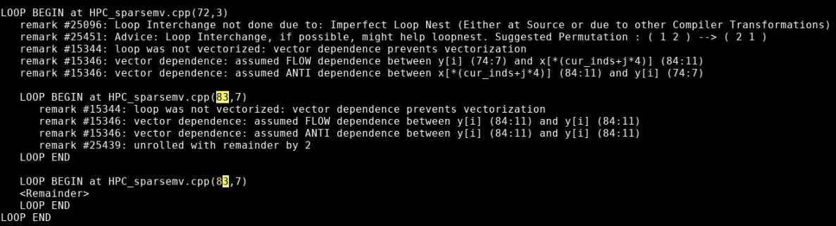
Incrementing a temporary variable instead of y[i], should enable vectorization:
for (int j=0; j< cur_nnz; j++)
  sum += cur_vals[j]*x[cur_inds[j]];
y[i] = sum;
Recompiling and rerunning with change reduces runtime from 74 seconds to 63 seconds.
Memory access is often the most important factor in your code's performance. Loops that work with arrays should use a stride of one whenever possible. C and C++ are row-major (store elements consecutively by row in 2D arrays), so the first array index should be the outermost loop and the last array index should be the innermost loop. Fortran is column-major, so the reverse is true. You can get factor of 3 or 4 speedup just by using unit stride. Avoid using arrays of derived data types, structs, or classes. For example, use structs of arrays instead of arrays of structures.
Efficient cache usage is important. Cache lines are 8 words (64 bytes) of consecutive memory. The entire cache line is loaded when a piece of data is fetched.
The code below is a good example. 2 cache lines are used for every 8 loop iterations, and it is unit stride:
real*8 a(N), b(N)
do i = 1,N
  a(i) = a(i) + b(i)
end do

! 2 cache lines:
! a(1), a(2), a(3) ... a(8)
! b(1), b(2), b(3) ... b(8)
The code below is a bad example. 1 cache line is loaded for each loop iteration, and it is not unit stride:
TYPE :: node
  real*8 a, b, c, d, w, x, y, z
END TYPE node
TYPE(node) :: s(N)
do i = 1, N
  s(i)%a = s(i)%a + s(i)%b
end do

! cache line:
! a(1), b(1), c(1), d(1), w(1), x(1), y(1), z(1)
Hands On
Look again at the most expensive parts of the code using ARM MAP:
module load arm-map
map -np 2 ./test_HPCCG 150 150 150
Look for any inefficient memory access patterns. Modify the code to improve memory access patterns and rerun the code. Do these changes improve performance?
Solution
Lines 110-148 of generate_matrix.cpp are nested loops:
for (int ix=0; ix<nx; ix++) {
  for (int iy=0; iy<ny; iy++) {
    for (int iz=0; iz<nz; iz++) {
      int curlocalrow = iz*nx*ny+iy*nx+ix;
      int currow = start_row+iz*nx*ny+iy*nx+ix;
      int nnzrow = 0;
      (*A)->ptr_to_vals_in_row[curlocalrow] = curvalptr;
      (*A)->ptr_to_inds_in_row[curlocalrow] = curindptr;
      .
      .
      .
    }
  }
}
The arrays are accessed in a manner so that consecutive values of ix are accesssed in order. However, our loops are ordered so that the ix is the outer loop. We can reorder the loops so that ix is iterated in the inner loop:
for (int iz=0; iz<nz; iz++) {
  for (int iy=0; iy<ny; iy++) {
    for (int ix=0; ix<nx; ix++) {
      .
      .
      .
    }
  }
}
This reduces the runtime from 63 seconds to 22 seconds.
OpenMP
OpenMP is a shared-memory, threaded parallel programming model. It is a portable standard with a set of compiler directives and a library of support functions. It is supported in compilers by Intel, Portland Group, GNU, and Cray.
The following are parallel loop execution examples in Fortran and C. The inner loop vectorizes while the outer loop executes on multiple threads:
PROGRAM omploop
INTEGER, PARAMETER :: N = 1000
INTEGER i, j
REAL, DIMENSION(N, N) :: a, b, c, x
... ! Initialize arrays
!$OMP PARALLEL DO
do j = 1, N
  do i = 1, N
    a(i, j) = b(i, j) + x(i, j) * c(i, j)
  end do
end do
!$OMP END PARALLEL DO
END PROGRAM omploop
int main() {
  int N = 1000;
  float *a, *b, *c, *x;
... // Allocate and initialize arrays
#pragma omp parallel for
  for (int i = 0; i < N; i++) {
    for (int j = 0; j < N; j++) {
      a[i*N+j] = b[i*N+j] + x[i*N+j] * c[i*N+j]
    }
  }
}
You can add an option to compile a program with OpenMP.
For Intel compilers, add the -qopenmp option. For example, ifort -qopenmp ompex.f90 -o ompex.
For GNU compilers, add the -fopenmp option. For example, gcc -fopenmp ompex.c -o ompex.
For Portland group compilers, add the -mp option. For example, pgf90 -mp ompex.f90 -o ompex.
To run an OpenMP program, requires multiple processors through Slurm (--N 1 -n 40) and set the OMP_NUM_THREADS environment variable (default is use all available cores). For the best performance, run at most one thread per core.
An example script is:
#!/bin/bash
#SBATCH -J omploop
#SBATCH -N 1
#SBATCH -n 40
#SBATCH -t 1:00

export OMP_NUM_THREADS=40
/usr/bin/time ./omploop
For more information, visit http://www.openmp.org, OpenMP Application Program Interface, and self-paced turorials. OSC will host an XSEDE OpenMP workshop on November 5, 2019.
MPI
MPI stands for message passing interface for when multiple processes run on one or more nodes. MPI has functions for point-to-point communication (e.g. MPI_Send, MPI_Recv). It also provides a number of functions for typical collective communication patterns, including MPI_Bcast (broadcasts value from root process to all other processes), MPI_Reduce (reduces values on all processes to a single value on a root process), MPI_Allreduce (reduces value on all processes to a single value and distributes the result back to all processes), MPI_Gather (gathers together values from a group of processes to a root process), and MPI_Alltoall (sends data from all processes to all processes).
A simple MPI program is:
#include <mpi.h>
#include <stdio.h>

int main(int argc, char *argv[]) {
  int rank, size;
  MPI_INIT(&argc, &argv);
  MPI_Comm_rank(MPI_COMM_WORLD, &rank);
  MPI_COMM_size(MPI_COMM_WORLD, &size);
  printf("Hello from node %d of %d\n", rank size);
  MPI_Finalize();
  return(0);
}
MPI implementations available at OSC are mvapich2, Intel MPI (only for Intel compilers), and OpenMPI.
MPI programs can be compiled with MPI compiler wrappers (mpicc, mpicxx, mpif90). They accept the same arguments as the compilers they wrap. For example, mpicc -o hello hello.c.
MPI programs must run in batch only. Debugging runs may be done with interactive batch jobs. srun automatically determines exectuion nodes from PBS:
#!/bin/bash
#SBATCH -J mpi_hello
#SBATCH -N 2
#SBATCH --ntasks-per-node=40
#SBATCH -t 1:00

cd $PBS_O_WORKDIR
srun ./hello
For more information about MPI, visit MPI Forum and MPI: A Message-Passing Interface Standard. OSC will host an XSEDE MPI workshop on September 3-4, 2019. Self-paced tutorials are available here.
Hands On
Use ITAC to get a timeline of the run of the code.
module load intelmpi
LD_PRELOAD=libVT.so \
mpiexec -trace -np 40 ./test_HPCCG 150 150 150
traceanalyzer <stf_file>
Look at the Event Timeline (under Charts). Do you see any communication patterns that could be replaced by a single MPI command?
Solution
Looking at the Event Timeline, we see that a large part of runtime is spent in the following communication pattern: MPI_Barrier, MPI_Send/MPI_Recv, MPI_Barrier. We also see that during this communication rank 0 is sending data to all other rank. We should be able to replace all of these MPI calls with a single call to MPI_Bcast.
The relavent code is in lines 82-89 of ddot.cpp:
  MPI_Barrier(MPI_COMM_WORLD);
  if(rank == 0) {
    for(int dst_rank=1; dst_rank < size; dst_rank++) {
      MPI_Send(&global_result, 1, MPI_DOUBLE, dst_rank, 1, MPI_COMM_WORLD);
    }
  }
  if(rank != 0) MPI_Recv(&global_result, 1, MPI_DOUBLE, 0, 1, MPI_COMM_WORLD, MPI_STATUS_IGNORE);
  MPI_Barrier(MPI_COMM_WORLD);
and can be replaced with:
MPI_Bcast(&global_result, 1, MPI_DOUBLE, 0, MPI_COMM_WORLD);
Interpreted Languages
Although many of the tools we already mentioned can also be used with interpreted languages, most interpreted languages such as Python and R have their own profiling tools.
Since they are still running on th same hardware, the performance considerations are very similar for interpreted languages as they are for compiled languages:
- Vectorization
- Efficient memory utilization
- Use built-in and library functions where possible
- Use appropriate data structures
- Understand and use best practices for the language
One of Python's most common profiling tools is cProfile. The simplest way to use cProfile is to add several arguments to your Python call so that an ordered list of the time spent in all functions called during executation. For instance, if a program is typically run with the command:
python ./mycode.py
replace that with
python -m cProfile -s time ./mycode.py
Here is a sample output from this profiler:
See Python's documentation for more details on how to use cProfile.
One of the most popular profilers for R is profvis. It is not available by default with R so it will need to be installed locally before its first use and loaded into your environment prior to each use. To profile your code, just put how you would usually call your code as the argument into profvis:
$ R
> install.packages('profvis')
> library('profvis')
> profvis({source('mycode.R')}
Here is a sample output from profvis:

For more information on profvis is available here.
Hands On
Python
First, enter the Python/ subdirectory of the code containing the python script ns.py. Profile this code with cProfile to determine the most expensive functions of the code. Next, rerun and profile with the array as an argument to ns.py. Which versions runs faster? Can you determine why it runs faster?
Solution
Execute the following commands:
python -m cProfile -s time ./ns.py
python -m cProfile -s time ./ns.py array
In the original code, 66 seconds out 68 seconds are spent in presPoissPeriodic. When the array argument is passed, the time spent in this function is approximately 1 second and the total runtime goes down to about 2 seconds.
The speedup comes from the vectorization of the main computation in the body of presPoissPeriodic by replacing nester for loops with a single like operation on arrays.
R
Now, enter the R/ subdirectory of the code containing the R script lu.R. Make sure that you have the R module loaded. First, run the code with profvis without any additional arguments and then again with frmt="matrix".
Which version of the code runs faster? Can you tell why it runs faster based on the profile?
Solution
Runtime for the default version is 28 seconds while the runtime when frmt="matrix" is 20 seconds.
Here is the profile with default arguments:
And here is the profile with frmt="matrix":

We can see that most of the time is being spent in lu_decomposition. The difference, however, is that the dataframe version seems to have a much higher overhead associated with accessing elements of the dataframe. On the other hand, the profile of the matrix version seems to be much flatter with fewer functions being called during LU decomposition. This reduction in overhead by using a matrix instead of a dataframe results in the better performance.
Tag:
Service:
Technologies:
HOWTO: Tune VASP Memory Usage
This article discusses memory tuning strategies for VASP.
Data Distribution
Typically the first approach for memory sensitive VASP issues is to tweak the data distribution (via NCORE or NPAR). The information at https://www.vasp.at/wiki/index.php/NPAR covers a variety of machines. OSC has fast communications via Infiniband.
Performance and memory consumption are dependent on the simulation model. So we recommend a series of benchmarks varying the number of nodes and NCORE. The recommended initial value for NCORE is the processor count per node which is the ntasks-per-node value in Slurm (the ppn value in PBS). Of course, if this benchmarking is intractable then one must reexamine the model. For general points see: https://www.vasp.at/wiki/index.php/Memory_requirements and https://www.vasp.at/wiki/index.php/Not_enough_memory And of course one should start small and incrementally improve or scale up one's model.
Rationalization
Using the key parameters with respect to memory scaling listed at the VASP memory requirements page one can rationalize VASP memory usage. The general approach is to study working calculations and then apply that understanding to scaled up or failing calculations. This might help one identify if a calculation is close to a node's memory limit and happens to cross over the limit for reasons that might be out of ones control, in which case one might need to switch to higher memory nodes.
Here is an example of rationalizing memory consumption. Extract from a simulation output the key parameters:
Dimension of arrays:
k-points NKPTS = 18 k-points in BZ NKDIM = 18 number of bands NBANDS= 1344
total plane-waves NPLWV = 752640
...
dimension x,y,z NGXF= 160 NGYF= 168 NGZF= 224
support grid NGXF= 320 NGYF= 336 NGZF= 448
This yields 273 GB of memory, NKDIM*NBANDS*NPLWV*16 + 4*(NGXF/2+1)*NGYF*NGZF*16, according to
https://www.vasp.at/wiki/index.php/Memory_requirements
This estimate should be compared to actual memory reports. See for example XDModD and grafana. Note that most application software has an overhead in the ballpack of ten to twenty percent. In addition, disk caching can consume significant memory. Thus, one must adjust the memory estimate upward. It can then be comapred to the available memory per cluster and per cluster node type.
Miscellaneous
- OSC sets the default resource limits for shells, except for core dump file size, to unlimited; see the limit/ulimit/unlimit commands depending on your shell.
- In the INCAR input file NWRITE=3 is for verbose output and NWRITE=4 is for debugging output.
- OSC does not have a VASP license and our staff has limited experience with it. So investigate alternate forms of help: ask within your research group and post on the VASP mailing list.
- Valgrind is a tool that can be used for many types of debugging including looking for memory corruptions and leaks. However, it slows down your code a very sizeable amount. This might not be feasible for HPC codes
- ASAN (address sanitizer) is another tool that can be used for memory debugging. It is less featureful than Valgrind, but runs much quicker, and so will likely work with your HPC code.
Service:
HOWTO: Use 'rclone' to Upload Data
rclone is a tool that can be used to upload and download files to a cloud storage (like Microsoft OneDrive, BuckeyeBox) from the command line. It's shipped as a standalone binary, but requires some user configuration before using. In this page, we will provide instructions on how to use rclone to upload data to OneDrive. For instructions with other cloud storage, check rclone Online documentation.
You can use "Globus" feature of OnDemand to perform data transfer between OneDrive and other storage. See this File Transfer and Management page for more information.
Setup
Before configuration, please first log into OSC OnDemand and request a Pitzer Lightweight Desktop session. Walltime of 1 hour should be sufficient to finish the configuration.
Note: this does not work with the 'konqueror' browser present on OSC Systems. Please set default to Firefox first before you do the setup following the instructions below:
* xfce: Applications (Top left corner) -> Settings -> Preferred Applications
* mate: System (top bar towards the left) -> Preferences -> Preferred Applications
* xfce: Applications (Top left corner) -> Settings -> Preferred Applications
* mate: System (top bar towards the left) -> Preferences -> Preferred Applications
Once the session is ready, open a terminal. In the terminal, run the command
rclone config
It prompts you with a bunch of questions:
- It shows "No remotes found -- make a new one" or list available remotes you made before
- Answer "n" for "New remote"
- "name>" (the name for the new remote)
- Type "OneDrive" (or whatever else you want to call this remote)
- "Storage>" (the storage type of the new remote)
- This should display a list to choose from. Enter the number corresponding to the "Microsoft OneDrive" storage type, which is "26".
- (It is "6" for BuckeyeBox)
- "client_id>"
- Leave this blank (just press enter).
- "client_secret>"
- Leave this blank (just press enter).
- "Choose national cloud region for OneDrive."
- This should display a list to choose from. Enter the number corresponding to the "Microsoft Cloud Global" region, which is "1".
- "Edit advanced config?"
- Type "n" for no
- "Use auto config?"
- Answer "y" for yes
- A web browser window should pop up allowing you to log into box. It is a good idea at this point to verify that the url is actually OneDrive before entering any credentials
- Enter your OSU email
- This should take you to the OSU login page. Login with your OSU credentials
- Go back to the terminal once "Success" is displayed.
- "Your choice>"
- One of five options to locate the drive you wish to use.
- Type "1" to use your personal or business OneDrive
- "Choose drive to use"
- Type "0"
- "Is this Okay? y/n>"
- Type "y" to confirm the drive you wish to use is correct.
- "y/e/d>"
- Type "y" to confirm you wish to add this remote to rclone.
Testing rclone
Note: you do not need to use Pitzer Lightweight Desktop when you run 'rclone'. You can test the data transfer with a small file using login nodes (i.e Pitzer), or request a regular compute node to do the data transfer with large files.
Create an empty hello.txt file and upload it to OneDrive using 'rclone copy' as below in a terminal:
touch hello.txt
rclone copy hello.txt OneDrive:/test
This creates a toplevel directory in OneDrive called 'test' if it does not already exist, and uploads the file hello.txt to it.
To verify the uploading is successful, you can either login to OneDrive in a web browser to check the file, or use rclone ls command in the terminal as:
rclone ls OneDrive:/test
Note: be careful when using
ls on a large directory, because it's recursive. You can add a '--max-depth 1' flag to stop the recursion. Downloading from OneDrive to OSC
Copy the contents of a source directory from a configured OneDrive remote, OneDrive:/src/dir/path, into a destination directory in your OSC session, /dest/dir/path, using the code below:
rclone copy OneDrive:/src/dir/path /dest/dir/path
Identical files on the source and destination directories are not transferred. Only the contents of the provided source directory are copied, not the directory name and contents.
copy does not delete files from the destination. To delete files from the destination directory in order to match the source directory, use the sync command instead.
If only one file is being transferred, use the copyto command instead.
Note: The
--no-traverse option can be used to increase efficiency by stopping rclone from listing the destination. It should be used when copying a small number of files and/or have a large number of files on the destination, but not when a large number of files are being copied.Note: Shared folders will not appear when listing a directory they are filed in. They are still accessible and data can be move to/from them. For example, the commands
rclone ls OneDrive:/path/to/shared_folder and rclone copy OneDrive:/path/to/shared_folder /dest/dir/path will work normally even though the shared folder does not appear when listing their source directory.Limitations
If rclone remains unused for 90 days, the refresh token will expire, leading to issues with authorization. This can be easily resolved by executing the rclone config reconnect remote: command, which generates a fresh token and refresh token.
Naming
It's important to note OneDrive is case insensitive which prohibits the coexistence files such as "Hello.doc" and "hello.doc". Certain characters are prohibited from being in OneDrive filenames and are commonly encountered on non-Windows platforms. Rclone addresses this by converting these filenames to their visually equivalent Unicode alternatives.
File Sizes
The largest allowed file size is 250 GiB for both OneDrive Personal and OneDrive for Business (Updated 13 Jan 2021).
Path Length
The entire path, including the file name, must contain fewer than 400 characters for OneDrive, OneDrive for Business and SharePoint Online. It is important to know the limitation when encrypting file and folder names with rclone, as the encrypted names are typically longer than the original ones.
Number of Files
OneDrive seems to be OK with at least 50,000 files in a folder, but at 100,000 rclone will get errors listing the directory like couldn’t list files: UnknownError:.
Reference
Supercomputer:
HOWTO: Use 'rclone' to Upload Data from Google Drive
rclone is a tool that can be used to upload and download files to a cloud storage (like Microsoft OneDrive) from the command line. It's shipped as a standalone binary, but requires some user configuration before using. In this page, we will provide instructions on how to use rclone to upload data from Google Drive. For instructions with other cloud storage, check rclone Online documentation.
Setup
Before configuration, please first log into OSC OnDemand and request a Pitzer Lightweight Desktop session. Walltime of 1 hour should be sufficient to finish the configuration.
Once the session is ready, open a terminal. In the terminal, run the command
rclone config
It prompts you with a bunch of questions:
- It shows "No remotes found -- make a new one" or list available remotes you made before
- Answer "n" for "New remote"
- "name>" (the name for the new remote)
- Type "GDrive" (or whatever else you want to call this remote)
- "Storage>" (the storage type of the new remote)
- This should display a list to choose from. Enter the number corresponding to the "Google Drive" storage type, which is "15".
- "client_id>"
- Leave this blank (just press enter).
- "client_secret>"
- Leave this blank (just press enter).
- Scope that rclone should use when requesting access from drive.
Enter a string value. Press Enter for the default ("").
Choose a number from below, or type in your own value- Select "2" for read-only access.
- ID of the root folder
- Leave this blank (just press enter)
- Service Account Credentials
- Leave this blank (just press enter)
- "Edit advanced config?"
- Type "n" for no
- "Use auto config?"
- Answer "y" for yes
- A web browser window should pop up allowing you to log into Google. It is a good idea at this point to verify that the URL is actually Google before entering any credentials. You may also copy and paste the link from Terminal into a web browser.
- Enter your Google credentials
- "Configure this as a Shared Drive (Team Drive)?"
- Answer "n" for no
Downloading from Google Drive to OSC
Copy the contents of a source directory from a configured OneDrive remote, GDrive:/src/dir/path, into a destination directory in your OSC session, /dest/dir/path, using the code below:
rclone copy GDrive:/src/dir/path /dest/dir/path --progress
Identical files on the source and destination directories are not transferred. Only the contents of the provided source directory are copied, not the directory name and contents.
copy does not delete files from the destination. To delete files from the destination directory in order to match the source directory, use the sync command instead.
If only one file is being transferred, use the copyto command instead.
Note: The
--no-traverse option can be used to increase efficiency by stopping rclone from listing the destination. It should be used when copying a small number of files and/or have a large number of files on the destination, but not when a large number of files are being copied.Note: Shared folders will not appear when listing a directory they are filed in. They are still accessible and data can be move to/from them. For example, the commands
rclone ls GDrive:/path/to/shared_folder and rclone copy GDrive:/path/to/shared_folder /dest/dir/path will work normally even though the shared folder does not appear when listing their source directory.Limitations
If rclone remains unused for 90 days, the refresh token will expire, leading to issues with authorization. This can be easily resolved by executing the rclone config reconnect remote: command, which generates a fresh token and refresh token.
Naming
It's important to note Google Drive is case insensitive which prohibits the coexistence files such as "Hello.doc" and "hello.doc". Certain characters are prohibited from being in Google Drive filenames and are commonly encountered on non-Windows platforms. Rclone addresses this by converting these filenames to their visually equivalent Unicode alternatives.
Reference
HOWTO: Use Address Sanitizer
Address Sanitizer is a tool developed by Google detect memory access error such as use-after-free and memory leaks. It is built into GCC versions >= 4.8 and can be used on both C and C++ codes. Address Sanitizer uses runtime instrumentation to track memory allocations, which mean you must build your code with Address Sanitizer to take advantage of it's features.
There is extensive documentation on the AddressSanitizer Github Wiki.
Memory leaks can increase the total memory used by your program. It's important to properly free memory when it's no longer required. For small programs, loosing a few bytes here and there may not seem like a big deal. However, for long running programs that use gigabytes of memory, avoiding memory leaks becomes increasingly vital. If your program fails to free the memory it uses when it no longer needs it, it can run out of memory, resulting in early termination of the application. AddressSanitizer can help detect these memory leaks.
Additionally, AddressSanitizer can detect use-after-free bugs. A use-after-free bug occurs when a program tries to read or write to memory that has already been freed. This is undefined behavior and can lead to corrupted data, incorrect results, and even program crashes.
Building With Address Sanitzer
We need to use gcc to build our code, so we'll load the gcc module:
module load gnu/9.1.0
The "-fsanitize=address" flag is used to tell the compiler to add AddressSanitizer.
Additionally, due to some environmental configuration settings on OSC systems, we must also statically link against Asan. This is done using the "-static-libasan" flag.
It's helpful to compile the code with debug symbols. AddressSanitizer will print line numbers if debug symbols are present. To do this, add the "-g" flag. Additionally, the "-fno-omit-frame-pointer" flag may be helpful if you find that your stack traces do not look quite correct.
In one command, this looks like:
gcc main.c -o main -fsanitize=address -static-libasan -g
Or, splitting into separate compiling and linking stages:
gcc -c main.c -fsanitize=address -g
gcc main.o -o main -fsanitize=address -static-libasan
Notice that both the compilation and linking steps require the "-fsanitize-address" flag, but only the linking step requires "-static-libasan". If your build system is more complex, it might make sense to put these flags in CFLAGS and LDFLAGS environment variables.
And that's it!
Examples
No Leak
First, let's look at a program that has no memory leaks (noleak.c):
#include <stdio.h>
#include <stdlib.h>
#include <string.h>

int main(int argc, const char *argv[]) {
    char *s = malloc(100);
    strcpy(s, "Hello world!");
    printf("string is: %s\n", s);
    free(s);
    return 0;
}
To build this we run:
gcc noleak.c -o noleak -fsanitize=address -static-libasan -g
And, the output we get after running it:
string is: Hello world!
That looks correct! Since there are no memory leaks in this program, AddressSanitizer did not print anything. But, what happens if there are leaks?
Missing free
Let's look at the above program again, but this time, remove the free call (leak.c):
#include <stdio.h>
#include <stdlib.h>
#include <string.h>

int main(int argc, const char *argv[]) {
    char *s = malloc(100);
    strcpy(s, "Hello world!");
    printf("string is: %s\n", s);
    return 0;
}
Then, to build:
gcc leak.c -o leak -fsanitize=address -static-libasan
And the output:
string is: Hello world!

=================================================================
==235624==ERROR: LeakSanitizer: detected memory leaks

Direct leak of 100 byte(s) in 1 object(s) allocated from:
    #0 0x4eaaa8 in __interceptor_malloc ../../.././libsanitizer/asan/asan_malloc_linux.cc:144
    #1 0x5283dd in main /users/PZS0710/edanish/test/asan/leak.c:6
    #2 0x2b0c29909544 in __libc_start_main (/lib64/libc.so.6+0x22544)

SUMMARY: AddressSanitizer: 100 byte(s) leaked in 1 allocation(s).
This is a leak report from AddressSanitizer. It detected that 100 bytes were allocated, but never freed. Looking at the stack trace that it provides, we can see that the memory was allocated on line 6 in leak.c
Use After Free
Say we found the above leak in our code, and we wanted to fix it. We need to add a call to free. But, what if we add it in the wrong spot?
#include <stdio.h>
#include <stdlib.h>
#include <string.h>

int main(int argc, const char *argv[]) {
    char *s = malloc(100);
    free(s);
    strcpy(s, "Hello world!");
    printf("string is: %s\n", s);
    return 0;
}
The above (uaf.c) is clearly wrong. Albiet a contrived example, the allocated memory, pointed to by "s", was written to and read from after it was freed.
To Build:
gcc uaf.c -o uaf -fsanitize=address -static-libasan
Building it and running it, we get the following report from AddressSanitizer:
=================================================================
==244157==ERROR: AddressSanitizer: heap-use-after-free on address 0x60b0000000f0 at pc 0x00000047a560 bp 0x7ffcdf0d59f0 sp 0x7ffcdf0d51a0
WRITE of size 13 at 0x60b0000000f0 thread T0
    #0 0x47a55f in __interceptor_memcpy ../../.././libsanitizer/sanitizer_common/sanitizer_common_interceptors.inc:790
    #1 0x528403 in main /users/PZS0710/edanish/test/asan/uaf.c:8
    #2 0x2b47dd204544 in __libc_start_main (/lib64/libc.so.6+0x22544)
    #3 0x405f5c  (/users/PZS0710/edanish/test/asan/uaf+0x405f5c)

0x60b0000000f0 is located 0 bytes inside of 100-byte region [0x60b0000000f0,0x60b000000154)
freed by thread T0 here:
    #0 0x4ea6f7 in __interceptor_free ../../.././libsanitizer/asan/asan_malloc_linux.cc:122
    #1 0x5283ed in main /users/PZS0710/edanish/test/asan/uaf.c:7
    #2 0x2b47dd204544 in __libc_start_main (/lib64/libc.so.6+0x22544)

previously allocated by thread T0 here:
    #0 0x4eaaa8 in __interceptor_malloc ../../.././libsanitizer/asan/asan_malloc_linux.cc:144
    #1 0x5283dd in main /users/PZS0710/edanish/test/asan/uaf.c:6
    #2 0x2b47dd204544 in __libc_start_main (/lib64/libc.so.6+0x22544)

SUMMARY: AddressSanitizer: heap-use-after-free ../../.././libsanitizer/sanitizer_common/sanitizer_common_interceptors.inc:790 in __interceptor_memcpy
Shadow bytes around the buggy address:
  0x0c167fff7fc0: 00 00 00 00 00 00 00 00 00 00 00 00 00 00 00 00
  0x0c167fff7fd0: 00 00 00 00 00 00 00 00 00 00 00 00 00 00 00 00
  0x0c167fff7fe0: 00 00 00 00 00 00 00 00 00 00 00 00 00 00 00 00
  0x0c167fff7ff0: 00 00 00 00 00 00 00 00 00 00 00 00 00 00 00 00
  0x0c167fff8000: fa fa fa fa fa fa fa fa fd fd fd fd fd fd fd fd
=>0x0c167fff8010: fd fd fd fd fd fa fa fa fa fa fa fa fa fa[fd]fd
  0x0c167fff8020: fd fd fd fd fd fd fd fd fd fd fd fa fa fa fa fa
  0x0c167fff8030: fa fa fa fa fa fa fa fa fa fa fa fa fa fa fa fa
  0x0c167fff8040: fa fa fa fa fa fa fa fa fa fa fa fa fa fa fa fa
  0x0c167fff8050: fa fa fa fa fa fa fa fa fa fa fa fa fa fa fa fa
  0x0c167fff8060: fa fa fa fa fa fa fa fa fa fa fa fa fa fa fa fa
Shadow byte legend (one shadow byte represents 8 application bytes):
  Addressable:           00
  Partially addressable: 01 02 03 04 05 06 07
  Heap left redzone:       fa
  Freed heap region:       fd
  Stack left redzone:      f1
  Stack mid redzone:       f2
  Stack right redzone:     f3
  Stack after return:      f5
  Stack use after scope:   f8
  Global redzone:          f9
  Global init order:       f6
  Poisoned by user:        f7
  Container overflow:      fc
  Array cookie:            ac
  Intra object redzone:    bb
  ASan internal:           fe
  Left alloca redzone:     ca
  Right alloca redzone:    cb
  Shadow gap:              cc
==244157==ABORTING
This is a bit intimidating. It looks like there's alot going on here, but it's not as bad as it looks. Starting at the top, we see what AddressSanitizer detected. In this case, a "WRITE" of 13 bytes (from our strcpy). Immediately below that, we get a stack trace of where the write occured. This tells us that the write occured on line 8 in uaf.c in the function called "main".
Next, AddressSanitizer reports where the memory was located. We can ignore this for now, but depending on your use case, it could be helpful information.
Two key pieces of information follow. AddressSanitizer tells us where the memory was freed (the "freed by thread T0 here" section), giving us another stack trace indicating the memory was freed on line 7. Then, it reports where it was originally allocated ("previously allocated by thread T0 here:"), line 6 in uaf.c.
This is likely enough information to start to debug the issue. The rest of the report provides details about how the memory is laid out, and exactly which addresses were accessed/written to. You probably won't need to pay too much attention to this section. It's a bit "down in the weeds" for most use cases.
Heap Overflow
AddresssSanitizer can also detect heap overflows. Consider the following code (overflow.c):
#include <stdio.h>
#include <stdlib.h>
#include <string.h>
int main(int argc, const char *argv[]) {
    // whoops, forgot c strings are null-terminated
    // and not enough memory was allocated for the copy
    char *s = malloc(12);
    strcpy(s, "Hello world!");
    printf("string is: %s\n", s);
    free(s);
    return 0;
}
The "Hello world!" string is 13 characters long including the null terminator, but we've only allocated 12 bytes, so the strcpy above will overflow the buffer that was allocated. To build this:
gcc overflow.c -o overflow -fsanitize=address -static-libasan -g -Wall
Then, running it, we get the following report from AddressSanitizer:
==168232==ERROR: AddressSanitizer: heap-buffer-overflow on address 0x60200000003c at pc 0x000000423454 bp 0x7ffdd58700e0 sp 0x7ffdd586f890
WRITE of size 13 at 0x60200000003c thread T0
    #0 0x423453 in __interceptor_memcpy /apps_src/gnu/8.4.0/src/libsanitizer/sanitizer_common/sanitizer_common_interceptors.inc:737
    #1 0x5097c9 in main /users/PZS0710/edanish/test/asan/overflow.c:8
    #2 0x2ad93cbd7544 in __libc_start_main (/lib64/libc.so.6+0x22544)
    #3 0x405d7b  (/users/PZS0710/edanish/test/asan/overflow+0x405d7b)

0x60200000003c is located 0 bytes to the right of 12-byte region [0x602000000030,0x60200000003c)
allocated by thread T0 here:
    #0 0x4cd5d0 in __interceptor_malloc /apps_src/gnu/8.4.0/src/libsanitizer/asan/asan_malloc_linux.cc:86
    #1 0x5097af in main /users/PZS0710/edanish/test/asan/overflow.c:7
    #2 0x2ad93cbd7544 in __libc_start_main (/lib64/libc.so.6+0x22544)

SUMMARY: AddressSanitizer: heap-buffer-overflow /apps_src/gnu/8.4.0/src/libsanitizer/sanitizer_common/sanitizer_common_interceptors.inc:737 in __interceptor_memcpy
Shadow bytes around the buggy address:
  0x0c047fff7fb0: 00 00 00 00 00 00 00 00 00 00 00 00 00 00 00 00
  0x0c047fff7fc0: 00 00 00 00 00 00 00 00 00 00 00 00 00 00 00 00
  0x0c047fff7fd0: 00 00 00 00 00 00 00 00 00 00 00 00 00 00 00 00
  0x0c047fff7fe0: 00 00 00 00 00 00 00 00 00 00 00 00 00 00 00 00
  0x0c047fff7ff0: 00 00 00 00 00 00 00 00 00 00 00 00 00 00 00 00
=>0x0c047fff8000: fa fa 00 fa fa fa 00[04]fa fa fa fa fa fa fa fa
  0x0c047fff8010: fa fa fa fa fa fa fa fa fa fa fa fa fa fa fa fa
  0x0c047fff8020: fa fa fa fa fa fa fa fa fa fa fa fa fa fa fa fa
  0x0c047fff8030: fa fa fa fa fa fa fa fa fa fa fa fa fa fa fa fa
  0x0c047fff8040: fa fa fa fa fa fa fa fa fa fa fa fa fa fa fa fa
  0x0c047fff8050: fa fa fa fa fa fa fa fa fa fa fa fa fa fa fa fa
Shadow byte legend (one shadow byte represents 8 application bytes):
  Addressable:           00
  Partially addressable: 01 02 03 04 05 06 07
  Heap left redzone:       fa
  Freed heap region:       fd
  Stack left redzone:      f1
  Stack mid redzone:       f2
  Stack right redzone:     f3
  Stack after return:      f5
  Stack use after scope:   f8
  Global redzone:          f9
  Global init order:       f6
  Poisoned by user:        f7
  Container overflow:      fc
  Array cookie:            ac
  Intra object redzone:    bb
  ASan internal:           fe
  Left alloca redzone:     ca
  Right alloca redzone:    cb
==168232==ABORTING
This is similar to the use-after-free report we looked at above. It tells us that a heap buffer overflow occured, then goes on to report where the write happened and where the memory was originally allocated. Again, the rest of this report describes the layout of the heap, and probably isn't too important for your use case.
C++ Delete Mismatch
AddressSanitizer can be used on C++ codes as well. Consider the following (bad_delete.cxx):
#include <iostream>
#include <cstring>

int main(int argc, const char *argv[]) {
    char *cstr = new char[100];
    strcpy(cstr, "Hello World");
    std::cout << cstr << std::endl;

    delete cstr;
    return 0;
}
What's the problem here? The memory pointed to by "cstr" was allocated with new[]. An array allocation must be deleted with the delete[] operator, not "delete".
To build this code, just use g++ instead of gcc:
g++ bad_delete.cxx -o bad_delete -fsanitize=address -static-libasan -g
And running it, we get the following output:
Hello World
=================================================================
==257438==ERROR: AddressSanitizer: alloc-dealloc-mismatch (operator new [] vs operator delete) on 0x60b000000040
    #0 0x4d0a78 in operator delete(void*, unsigned long) /apps_src/gnu/8.4.0/src/libsanitizer/asan/asan_new_delete.cc:151
    #1 0x509ea8 in main /users/PZS0710/edanish/test/asan/bad_delete.cxx:9
    #2 0x2b8232878544 in __libc_start_main (/lib64/libc.so.6+0x22544)
    #3 0x40642b  (/users/PZS0710/edanish/test/asan/bad_delete+0x40642b)

0x60b000000040 is located 0 bytes inside of 100-byte region [0x60b000000040,0x60b0000000a4)
allocated by thread T0 here:
    #0 0x4cf840 in operator new[](unsigned long) /apps_src/gnu/8.4.0/src/libsanitizer/asan/asan_new_delete.cc:93
    #1 0x509e5f in main /users/PZS0710/edanish/test/asan/bad_delete.cxx:5
    #2 0x2b8232878544 in __libc_start_main (/lib64/libc.so.6+0x22544)

SUMMARY: AddressSanitizer: alloc-dealloc-mismatch /apps_src/gnu/8.4.0/src/libsanitizer/asan/asan_new_delete.cc:151 in operator delete(void*, unsigned long)
==257438==HINT: if you don't care about these errors you may set ASAN_OPTIONS=alloc_dealloc_mismatch=0
==257438==ABORTING
This is similar to the other AddressSanitizer outputs we've looked at. This time, it tells us there's a mismatch between new and delete. It prints a stack trace for where the delete occured (line 9) and also a stack trace for where to allocation occured (line 5).
Performance
The documentation states:
This tool is very fast. The average slowdown of the instrumented program is ~2x
AddressSanitizer is much faster than tools that do similar analysis such as valgrind. This allows for usage on HPC codes.
However, if you find that AddressSanitizer is too slow for your code, there are compiler flags that can be used to disable it for specific functions. This way, you can use address sanitizer on cooler parts of your code, while manually auditing the hot paths.
The compiler directive to skip analyzing functions is:
__attribute__((no_sanitize_address)
Technologies:
HOWTO: Use Cron and OSCusage for Regular Emailed Reports
It is possible to utilize Cron and the OSCusage command to send regular usage reports via email
Cron
It is easy to create Cron jobs on the Cardinal and Pitzer clusters at OSC. Cron is a Linux utility which allows the user to schedule a command or script to run automatically at a specific date and time. A cron job is the task that is scheduled.
Shell scripts run as a cron job are usually used to update and modify files or databases; however, they can perform other tasks, for example a cron job can send an email notification.
Getting Help
In order to use what cron has to offer, here is a list of the command name and options that can be used
Usage: crontab [options] file crontab [options] crontab -n [hostname] Options: -udefine user -e edit user's crontab -l list user's crontab -r delete user's crontab -i prompt before deleting -n set host in cluster to run users' crontabs -c get host in cluster to run users' crontabs -s selinux context -x enable debugging
Running a Cron Job
crontab -l
crontab -e
Linux Crontab Format
MIN HOUR DOM MON DOW CMD

Getting Notified by Email Using a Cron Job
* * * * * {cmd} | mail -s "title of the email notification" {your email}
12 15 * * * /opt/osc/bin/OSCusage | mail -s "OSC usage on $(date)" {your email} 2> /path/to/file/for/stdout/and/stderr 2>&1
Using OSCusage
$ /opt/osc/bin/OSCusage --help
usage: OSCusage.py [-h] [-u USER]
[-s {opt,pitzer,glenn,bale,oak,oakley,owens,ruby,ascend,cardinal}] [-A]
[-P PROJECT] [-q] [-H] [-r] [-n] [-v]
[start_date] [end_date]

positional arguments:
start_date start date (default: 2020-04-23)
end_date end date (default: 2020-04-24)

optional arguments:
-h, --help show this help message and exit
-u USER, --user USER username to run as. Be sure to include -P or -A. (default: kalattar)
-s {opt,pitzer,glenn,bale,oak,oakley,owens,ruby,ascend,cardinal}, --system {opt,pitzer,glenn,bale,oak,oakle
-A Show all
-P PROJECT, --project PROJECT project to query (default: PZS0715)
-q show user data
-H show hours
-r show raw
-n show job ID
-v do not summarize
OSCusage 2018-01-24
OSCusage 2018-01-24 2018-01-25
Terminating a Cron Job
ps aux | grep crontab
kill {PID}
crontab -e
HOWTO: Use Docker and Singularity Containers at OSC
It is now possible to run Docker and Apptainer/Singularity containers on all clusters at OSC. Single-node jobs are currently supported, including GPU jobs; MPI jobs are planned for the future.
From the Docker website: "A container image is a lightweight, stand-alone, executable package of a piece of software that includes everything needed to run it: code, runtime, system tools, system libraries, settings."
As of June 21st, 2022, Singularity is replaced with Apptainer, which is just a renamed open-source project. For more information visit the Apptainer/Singularity page
This document will describe how to run Docker and Apptainer/Singularity containers on OSC clusters. You can use containers from Docker Hub, Sylabs Cloud, or any other source. As examples we will use hello-world and ubuntu from Docker Hub.
If you encounter an error then check the Known Issues on using Apptainer/Singularity or Podman at OSC. If the issue can not be resolved, please contact OSC help.
Contents
- Getting help
- Setting up your environment
- Accessing a container
- Running a container
- File system access
- GPU usage within a container
- Build a container
- Known issues
- References
Getting help
-
For Apptainer/Singularity, use
apptainer help. -
For Podman/Docker, use
podman help. -
User guides and examples are available at Podman documentation and Apptainer documentation.
Setting up your environment for Podman or Apptainer/Singularity usage
No setup is required. You can use Podman or Apptainer/Singularity directly on all clusters.
Accessing a container
A container image is a file (e.g. .sif for Apptainer) or image stored in a registry (for Docker/Podman).
You can pull images from hubs: Docker Hub, Sylabs Cloud, or other registries.
Using Apptainer/Singularity
Examples:
# Pull the gcc:7.2.0 image from Docker Hub → gcc_7.2.0.sif
apptainer pull docker://gcc:7.2.0

# Ubuntu 18.04 → ubuntu_18.04.sif
apptainer pull docker://ubuntu:18.04

# Pull from Singularity Hub
apptainer pull shub://singularityhub/hello-world
Downloading Apptainer/Singularitycontainers from the hubs is not the only way to get one. You can, for example get a copy from your colleague's computer or directory. If you would like to create your own container you can start from the Build a container section below. If you have any questions, please contact OSC Help.
Using Podman/Docker
With Podman/Docker, you pull images to your local image store:
podman pull ubuntu:18.04
podman pull docker.io/library/gcc:7.2.0
Use podman images to list available images in the local registry:
REPOSITORY                TAG         IMAGE ID      CREATED      SIZE
docker.io/library/ubuntu  18.04       f9a80a55f492  2 years ago  65.5 MB
docker.io/library/gcc     7.2.0       81ffb25b1dec  7 years ago  1.73 GB
Running a container
You can run containers on OSC clusters either interactively or in batch jobs.
IMPORTANT: Don’t run on a login node if the container will be performing heavy computation, of course.
If unsure about the amount of memory that a singularity process will require, then be sure to request an entire node for the job. It is common for singularity jobs to be killed by the OOM killer because of using too much RAM.
If unsure about the amount of memory that a singularity process will require, then be sure to request an entire node for the job. It is common for singularity jobs to be killed by the OOM killer because of using too much RAM.
We note that the operating system on OSC cluster is Red Hat by running cat /etc/os-release:
NAME="Red Hat Enterprise Linux Server"
[..more..]
In the examples below we will often check the operating system to show that we are really inside a container.
Using Apptainer/Singularity
Run container like a native command
If you simply run the container image, it will execute the container’s runscript.
apptainer pull docker://hello-wolrd
./hello-world_latest.sif
You should see the following output:
Hello from Docker!
This message shows that your installation appears to be working correctly.
Use the “run” sub-command
The Apptainer “run” sub-command does the same thing as running a container directly as described above. That is, it executes the container’s runscript.
Example: Run a container from a local file
apptainer run hello-world_latest.sif
Example: Run a container from a hub without explicitly downloading it
apptainer run docker://hello-world
Use the “exec” sub-command
The Apptainer “exec” sub-command lets you execute an arbitrary command within your container instead of just the runscript.
Example: Find out what operating system the ubuntu:18.04 container uses
apptainer pull docker://ubuntu:18.04
apptainer exec ./ubuntu_18.04.sif cat /etc/os-release
You should see the following output:
NAME="Ubuntu"
VERSION="18.04.6 LTS (Bionic Beaver)"
Use the “shell” sub-command
The Apptainer “shell” sub-command invokes an interactive shell within a container.
Example: Run an Ubuntu shell.
apptainer shell ubuntu_18.04.sif
You should now see the prompt Apptainer>, indicating that you are logged into the container. You can verify the operating system version by running:
Apptainer> cat /etc/os-release
Output:
NAME="Ubuntu"
VERSION="18.04.6 LTS (Bionic Beaver)"
To exit the container, simply type exit.
Using Podman/Docker
With Podman or Docker:
-
Run: runs the container’s default command
podman run hello-world
-
Exec: execute arbitrary command inside running (or started) container
podman run -t -d --name my_ubuntu ubuntu:18.04
podman exec my_ubuntu cat /etc/os-release
-
Interactive shell:
podman run -it ubuntu:18.04
File system access
Using Apptainer/Singularity
When you use a container you run within the container’s environment. The directories available to you by default from the host environment are
- your home directory
- working directory (directory you were in when you ran the container)
/fs/ess/tmp
You can review our Available File Systems page for more details about our file system access policy.
If you run the container within a job you will have the usual access to the $PFSDIR environment variable with adding node attribute "pfsdir" in the job request (--gres=pfsdir). You can access most of our file systems from a container without any special treatment.
Using Podman/Docker
If using Podman/Docker, you may need to explicitly bind mount host directories into the container. For example:
podman run -it -v $HOME:$HOME -v /fs/ess:/fs/ess $ubuntu:18.04
GPU usage within a container
Using Apptainer/Singularity
If you have a GPU-enabled container you can easily run it on Pitzer just by adding the --nv flag to the apptainer exec or run command. The example below comes from the "exec" command section of Apptainer User Guide. It runs a TensorFlow example using a GPU on Pitzer. (Output has been omitted from the example for brevity.)
[pitzer-login01]$ salloc -N 1 --ntasks-per-node=4 -G 1...[p0756]$git clone https://github.com/tensorflow/models.git[p0756]$apptainer exec --nv docker://tensorflow/tensorflow:latest-gpu \ python ./models/tutorials/image/mnist/convolutional.py
In some cases it may be necessary to bind the CUDA_HOME path and add $CUDA_HOME/lib64 to the shared library search path:
[pitzer-login01]$ salloc -N 1 --ntasks-per-node=4 -G 1...[p0756]$module load cuda [p0756]$ export APPTAINER_BINDPATH=$CUDA_HOME [p0756]$ export APPTAINERENV_LD_LIBRARY_PATH=$LD_LIBRARY_PATH:$CUDA_HOME/lib64[p0756]$napptainer exec --nv my_container mycmd
Using Podman/Docker
To use a GPU in a Docker container, you need to add the GPU device using the --device option.
For example, to request a GPU node with one GPU:
salloc -n 1 -G 1
After obtaining the node, you can test if the GPU device is available in a container by running:
podman run --rm --device nvidia.com/gpu=all nvidia/cuda:11.0.3-base-ubuntu20.04 nvidia-smi
If successful, the nvidia-smi command will display details about the GPU, such as model, memory usage, and driver version.
Build a container
Using Apptainer/Singularity
OSC users can now build an Apptainer/Singularity container image from a definition file using the fakeroot feature:
apptainer build --fakeroot myimage.sif mydef.def
When building an image, it is recommended to change the cache folder (the default location is $HOME/.apptainer/cache) to improve build efficiency and avoid potential file system issues, especially when building a large container image.
Recommended steps
Request a compute node with sufficient memory. The following example requests a compute node with 32 GB of memory:
sinteractive -n 8
Change the cache folder to a temporary file system:
export APPTAINER_CACHEDIR=$TMPDIR
Build an image:
apptainer build --fakeroot myimage.sif mydef.def
These steps help optimize performance and prevent file system issues when building large container images.
Using Podman/Docker
OSC users can now build a Docker container image from a Dockerfile:
buildah build -f Dockerfile --format docker -t tag_my_container .
The option --format docker ensures that the container format is compatible with the Docker schema for the manifest. The -t flag is used to tag the image, typically in the format name:version.
For example, if you set -t my_container:1.0, you should see the following after listing images with podman images:
REPOSITORY                TAG         IMAGE ID      CREATED      SIZE
local/my_container        1.0         f9a80a55f492  30 mins ago  65.5 MB
Note that our local registry is saved on a local disk. This means that if you build an image on a compute node, it will not be accessible from other nodes and will be removed once the job ends.
To ensure that your container image can be reused, you should create an account on Docker Hub (or another supported container registry) and tag your image with the registry URL. For example:
podman login
podman tag my_container:1.0 docker.io/<username>/my_container:1.0
podman push docker.io/<username>/my_container:1.0
Known isues
References
Service:
HOWTO: Use Extensions with JupyterLab
JupyterLab stores the main build of JupyterLab with associated data, including extensions in Application Directory. The default Application Directory is the JupyterLab installation directory where is read-only for OSC users. Unlike Jupyter Notebook, JupyterLab cannot accommodate multiple paths for extensions management. Therefore we set the user's home directory for Application Directory so as to allow user to manage extensions.
NOTE: The extension management is only available for JupyterLab 2 or later.
Manage and install extensions
After launching a JupyterLab session, open a notebook and run
!jupyter lab path
Check if home directory is set for to the Application Directory
Application directory:   /users/PXX1234/user/.jupyter/lab/3.0
User Settings directory: /users/PXX1234/user/.jupyter/lab/user-settings
Workspaces directory: /users/PXX1234/user/ondemand/data/sys/dashboard/batch_connect/dev/bc_osc_jupyter/output/f2a4f918-b18c-4d2a-88bc-4f4e1bdfe03e
If home directory is NOT set, try removing the corresonding directory, e.g. if you are using JupyterLab 2.2, remove the entire directory $HOME/.jupyter/lab/2.2 and re-launch JupyterLab 2.2.
If this is the first time to use extension or use extensions that are installed with different Jupyter version or on different cluster, you will need to run
!jupyter lab build
to initialize the JupyterLab application.
To manage and install extensions, simply click Extension Manager icon at the side bar:
Please note that OSC Jupyter app is a portal to launch JupyterLab installed on OSC. It does not act the same as the standalone Jupyter installed on your computer. Some extensions that work on your computer might not work with OSC Jupyter. If you experience any issue, please contact OSC help.
Service:
HOWTO: Use GPU in Python
If you plan on using GPUs in tensorflow or pytorch see HOWTO: Use GPU with Tensorflow and PyTorch
This is an exmaple to utilize a GPU to improve performace in our python computations. We will make use of the Numba python library. Numba provides numerious tools to improve perfromace of your python code including GPU support.
This tutorial is only a high level overview of the basics of running python on a gpu. For more detailed documentation and instructions refer to the official numba document: https://numba.pydata.org/numba-doc/latest/cuda/index.html
Environment Setup
To begin, you need to first create and new conda environment or use an already existing one. See HOWTO: Create Python Environment for more details.
Once you have an environment created and activated run the following command to install the latest version of Numba into the environment.
conda install numba
conda install cudatoolkit
You can specify a specific version by replacing numba with number={version}. In this turtorial we will be using numba version 0.60.0 and cudatoolkit version 12.3.52.
Write Code
Now we can use numba to write a kernel function. (a kernel function is a GPU function that is called from CPU code).
To invoke a kernel, you need to include the @cuda.jit decorator above your gpu function as such:
@cuda.jit
def my_funtion(array):
     # function code
Next to invoke a kernel you must first specify the thread heirachy with the number of blocks per grid and threads per block you want on your gpu:
threadsperblock = 32
blockspergrid = (an_array.size + (threadsperblock - 1))
For more details on thread heirachy see: https://numba.pydata.org/numba-doc/latest/cuda/kernels.html
Now you can call you kernel as such:
my_function[blockspergrid, threadsperblock](an_array)
Kernel instantiation is done by taking the compiled kernel function (here my_function) and indexing it with a tuple of integers.
Run the kernel, by passing it the input array (and any separate output arrays if necessary). By default, running a kernel is synchronous: the function returns when the kernel has finished executing and the data is synchronized back.
Note: Kernels cannot explicitly return a value, as a result, all returned results should be written to a reference. For example, you can write your output data to an array which was passed in as an argument (for scalars you can use a one-element array)
Memory Transfer
Before we can use a kernel on an array of data we need to transfer the data from host memory to gpu memory.
This can be done by (assume arr is already created and filled with the data):
d_arr = cuda.to_device(arr)
d_arr is a reference to the data stored in the gpu memory.
Now to get the gpu data back into host memory we can run (assume gpu_arr has already been initialized ot an empty array):
d_arr.copy_to_host(gpu_arr)
Example Code:
from numba import cuda
import numpy as np
from timeit import default_timer as timer

# gpu kernel function
@cuda.jit
def increment_by_one_gpu(an_array):
    #get the absolute position of the current thread in out 1 dimentional grid
    pos = cuda.grid(1)

    #increment the entry in the array based on its thread position
    if pos < an_array.size:
        an_array[pos] += 1


# cpu function
def increment_by_one_nogpu(an_array):
    # increment each position using standard iterative approach
    pos = 0
    while pos < an_array.size:
        an_array[pos] += 1
        pos += 1

if __name__ == "__main__":

    # create numpy array of 10 million 1s
    n = 10_000_000
    arr = np.ones(n)

    # copy the array to gpu memory
    d_arr = cuda.to_device(arr)

    # print inital array values
    print("GPU Array: ", arr)
    print("NON-GPU Array: ", arr)

    #specify threads
    threadsperblock = 32
    blockspergrid = (len(arr) + (threadsperblock - 1)) // threadsperblock

    # start timer
    start = timer()
    # run gpu kernel
    increment_by_one_gpu[blockspergrid, threadsperblock](d_arr)
    # get time elapsed for gpu
    dt = timer() - start

    print("Time With GPU: ", dt)

    # restart timer
    start = timer()
    # run cpu function
    increment_by_one_nogpu(arr)
    # get time elapsed for cpu
    dt = timer() - start

    print("Time Without GPU: ", dt)

    # create empty array
    gpu_arr = np.empty(shape=d_arr.shape, dtype=d_arr.dtype)

    # move data back to host memory
    d_arr.copy_to_host(gpu_arr)

    print("GPU Array: ", gpu_arr)
    print("NON-GPU Array: ", arr)
Now we need to write a job script to submit the python code.
Make sure you request a gpu for your job! See GPU Computing for more details.
#!/bin/bash

#SBATCH --account <project-id>
#SBATCH --job-name Python_ExampleJob
#SBATCH --nodes=1
#SBATCH --time=00:10:00
#SBATCH --gpus-per-node=1


module load miniconda3/24.1.2-py310
module list

source activate gpu_env

python gpu_test.py

conda deactivate
Running the above job returns the following output:
GPU Array:  [1. 1. 1. ... 1. 1. 1.]
NON-GPU Array:  [1. 1. 1. ... 1. 1. 1.]
Time With GPU:  0.34201269410550594
Time Without GPU:  2.2052815910428762
GPU Array:  [2. 2. 2. ... 2. 2. 2.]
NON-GPU Array:  [2. 2. 2. ... 2. 2. 2.]
As we can see, running the function on a gpu resulted in a signifcant speed increase.
Usage on Jupyter
see HOWTO: Use a Conda/Virtual Environment With Jupyter for more information on how to setup jupyter kernels.
One you have your jupyter kernel created, activate your python environment in the command line (source activate ENV).
Install numba and cudatoolkit the same as was done above:
conda install numba
conda install cudatoolkit
Now you should have numba installed into your jupyter kernel.
See Python page for more information on how to access your jupyter notebook on OnDemand.
Make sure you select a node with a gpu before laucnhing your jupyter app:

Additional Resources
If you are using Tensorflow, PyTorch or other machine learning frameworks you may want to also consider using Horovod. Horovod will take single-GPU training scripts and scale it to train across many GPUs in parallel.
HOWTO: Use Globus (Overview)
![]()
Globus is a cloud-based service designed to let users move, share, and discover research data via a single interface, regardless of its location or number of files or size.
Globus was developed and is maintained at the University of Chicago and is used extensively at supercomputer centers and major research facilities.
Globus is available as a free service that any user can access. More on how Globus works can be found on the Globus "How It Works" page.
Data Transfer
Globus can be used to transfer data between source and destination systems including OSC storage, cloud storage, storage at other HPC centers with Globus support, laptops, desktops.
If you would like to transfer data between OSC storage and your own laptop/desktop which has not installed Globus Connect Personal yet, please go to 'Globus Connect Personal Installation' first
Step 1: Log into Globus
Log into https://www.globus.org/
When prompted to login, select "Ohio Supercomputer Center (OSC)" from the drop-down list of organizations and then click Continue. This will redirect you to the Ohio Supercomputer Center login page where you can log in with your OSC username and password.
Step 2: Locate collections of your data
Click 'File Manager' on the left of the page. Switch to 'two panel' view by clicking the appropriate icon next to 'Panels' in the top right corner. One panel will act as the source while the other is the destination.
In each panel, you can click 'Collection' to search and select the appropriate collection.
To find your local collection (the one created via Globus Connect Personal), you can use the 'Your Collections' tab.
To locate the correct collection from OSC storage, please see 'OSC endpoints'.
Step 3: Transfer the file
Select the file(s) or directory that you would like to transfer between collections.
Click the "Transfer or Sync to..." button in the center control panel (two diagonal arrows).
Click the blue "Start" button above the file selector.
A ribbon should appear that recognizes the transfer request. You can hit View Details to take you to the Activity tab in the command menu.
Step 4: Verify the transfer
Click Activity in the command menu on the left of the page to go to the Activity page.
A green checkmark will appear at the top of the page with a Transfer Complete Message.
The email you have set up with your Globus profile will receive a confirmation receipt of the request.
The files will now be accessible in the transfer location.
Globus Connect Personal Installation
Globus Installation on Windows
-
Launch the application installer.
-
If you have local administrator permissions on your machine, and will be the only user, click on 'Install'.
- If you do not have local administrator permissions or wish to specify a non-default destination directory for installation, or will have multiple GCP users, click on the 'Browse' button and select a directory which you have read/write access to.
- If you do not have local administrator permissions or wish to specify a non-default destination directory for installation, or will have multiple GCP users, click on the 'Browse' button and select a directory which you have read/write access to.
-
After installation has completed GCP will launch. Click on 'Log In' in order to authenticate with Globus and begin the Collection Setup process.
-
Grant the required consents to GCP Setup.
-
Enter the details for your GCP Collection.
-
Exit the Setup process or open the Globus web app to view collection details or move data to or from your collection.
-
At the end of the installation, you will see an icon in the menu bar at the bottom of your screen, indicating that Globus Connect Personal is running and your new collection is ready to be used.
OSC Endpoints
- Enter 'OSC Globus Connect Server' in the endpoint search box to find all the endpointss managed by OSC as below:
| Endpoint | |
|---|---|
| OSC's home directory | OSC $HOME |
| OSC's scratch directory | OSC /fs/scratch |
| OSC's ess storage | OSC /fs/ess |
| AWS S3 storage | OSC S3 |
| OSC high assurance |
OSC /fs/ess/ High Assurance for project storage OSC /fs/scratch/ High Assurance for scratch storage |
Note: the default path will be $HOME for home directory, /fs/ess for project storage, /fs/scratch for scratch filesystem. You can change to a more specific directory by providing the path in ‘Directory’. The location for project/scratch data would be under /fs/ess/<project-code> or /fs/scratch/<project-code>.
Globus Connectors
Globus connectors provide a consistent interface for accessing, transferring, and sharing data across a wide range of storage systems. OSC has acquired all available connectors including AWS S3, dropbox, with the exception of the HPSS connector. For a complete list of connectors, please visit the Globus connectors page.
Data Sharing
With Globus, you can easily share research data with your collaborators. You don’t need to create accounts on the server(s) where your data is stored. You can share data with anyone using their identity or their email address.
To share data, you’ll create a guest collection and grant your collaborators access as described in the instructions below. If you like, you can designate other Globus users as "access managers" for the guest collection, allowing them to grant or revoke access privileges for other Globus users.
-
Log into Globus and navigate to the File Manager.
-
Select the collection that has the files/folders you wish to share and, if necessary, activate the collection.
-
Highlight the folder that you would like to share and Click Share in the right command pane.
Note: Sharing is available for folders. Individual files can only be shared by sharing the folder that contains them. If you are using an ad blocker plugin in your browser, the share button may be unavailable. We recommend users whitelist app.globus.org, docs.globus.org, and globus.org within the plugin to circumvent this issue.If Share is not available, contact the endpoint’s administrator or refer to Globus Connect Server Installation Guide for instructions on enabling sharing. If you’re a using a Globus Connect Personal endpoint and you’re a Globus Plus user, enable sharing by opening the Preferences for Globus Connect Personal, clicking the Access tab, and checking the Sharable box.
-
Provide a name for the guest collection, and click Create Share. If this is the first time you are accessing the collection, you may need to authenticate and consent to allow Globus services to manage your collections on your behalf.
-
When your collection is created, you’ll be taken to the Sharing tab, where you can set permissions. The starting permissions give read and write access (and the Administrator role) to the person who created the collection.
Click the Add Permissions button or icon to share access with others. You can add permissions for an individual user, for a group, or for all logged-in users. In the Identity/E-mail field, type a person’s name or username (if user is selected) or a group name (if group is selected) and press Enter. Globus will display matching identities. Pick from the list. If the user hasn’t used Globus before or you only have an email address, enter the email address and click Add.
Note: Granting write access to a folder allows users to modify and delete files and folders within the folder.You can add permissions to subfolders by entering a path in the Path field.
-
After receiving the email notification, your colleague can click on the link to log into Globus and access the guest collection.
-
You can allow others to manage the permissions for a collection you create. Use the Roles tab to manage roles for other users. You can assign roles to individual users or to groups. The default is for the person who created the collection to have the Administrator role.
The Access Manager role grants the ability to manage permissions for a collection. (Users with this role automatically have read/write access for the collection.)
When a role is assigned to a group, all members of the group have the assigned role.
Data Sharing with Service Account
Sometimes, a group may need to share data uploaded by several OSC users with external entities using Globus. To simplify this process OSC can help set up a service account that owns the data and create a Globus share that makes the data accessible to individuals. Contact OSC Help for this service.
Further Reading
HOWTO: Use AWS S3 in Globus
Beofre creating a new collection, please set up a S3 bucket and configure the IAM access permissions to that bucket. If you need more information on how to do that, see the AWS S3 documentation and Amazon Web Services S3 Connector pages.
Create a New Collection
- Login to Globus. If your institution does not have an organizational login, you may choose to either Sign in with Google or Sign in with ORCiD iD
- Navigate to the 'COLLECTIONS' on the sidebar and search 'OSC S3'. Click 'OSC S3' to go to this gateway
- Click on the “Credentials” tab of the “OSC S3” page. Register your AWS IAM access key ID and AWS IAM Secret Key with Globus. Click the “Continue” button, and you will return to the full “Credentials” tab where you can see your saved AWS access credentials.
- Click on the 'Collections' tab. You will see all of the collections added by you before. To add a new collection, click 'Add Guest Collection'. Click the “Browse” button to get a directory view and select the bucket or subfolder folder you want. Provide the name of the collection in 'Display Name” field
- Click 'Create Collection' to finish the creation
- Click 'COLLECTIONS' on the sidebar. Click the 'Administered by You' and then you can locate the new collection you just created.
HOWTO: Use OneDrive in Globus
Accessing User OneDrive in Globus
Globus is a cloud-based service designed to let users move, share, and discover research data via a single interface, regardless of its location or number of files or size.
This makes Globus incredibly useful for transferring large files for users. This service is also able to work alongside OneDrive, making your this storage even more attainable. The OneDrive connection to Globus is only available for Ohio State clients with a valid OSU email.
Data Transfer with OneDrive
Step 1: Log into Globus
Log into https://www.globus.org/
When prompted to login, select "Ohio Supercomputer Center (OSC)" from the drop-down list of organizations and then click Continue. This will redirect you to the Ohio Supercomputer Center login page where you can log in with your OSC username and password.
Step 2: Choose the Appropriate Collections
Select the File Manager tab on the left hand toolbar. You will be introduced to the file exchange function in the two-panel format.

In the left panel, select the collection that you would like to import the data to. In the right panel, you can simply type "OSU OneDrive" or "OSU OneDrive Student" and the collection will appear. Students will need to use their buckeyemail.osu.edu emails in order to access the student OneDrive.
The first time that you access this collection, you will be prompted for some initial account setup.

Complete the Authentication Request and, if prompted, verify that you wish to grant access to the Collection.
Once opened, the default location will be My Files. Click the "up one folder" icon to see the other locations.
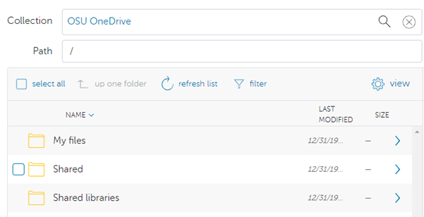
Step 3: Transfer the Files
Select the file(s) or directory that you would like to transfer between collections. You can now select the "Transfer or Sync to..." and hit the blue "Start" icon above the file selector.
Step 4: Verify the transfer
Click Activity in the command menu on the left of the page to go to the Activity page. You will now be able to monitor the processing of the request and the confirmation receipt will appear here.
Following Sites in SharePoint
To follow a SharePoint site, log into the OSU SharePoint service with your OSC name.# credentials. Next, navigate to the site you would like to connect to via Globus and click the star icon on the site to follow:
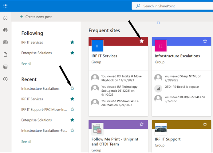
Finally, return to Globus and click the "up one folder" button until you see the "Shared libraries" and the SharePoint site will now be available.
HOWTO: Deploy your own endpoint on a server
OSC clients who are affiliated with Ohio State can deploy their own endpoint on a server using OSU subscriptions. Please follow the steps below:
- Send a request to OSC Help the following information:
- Name of organization that will be running the endpoint, ie: OSU Arts and Sciences
- NOTE: if the name already exists, they will have to coordinate with the existing Admin for that project
- OSU affiliated email address associated with the Globus account, ie: name.#@osu.edu
- Name of organization that will be running the endpoint, ie: OSU Arts and Sciences
- OSC will create a new project at https://developers.globus.org, make the user provided in #1 the administrator, and inform the user to set up the endpoint credentials
- The user goes to https://developers.globus.org/ and chooses “Register a new Globus Connect Server v5”. Under the project, the user chooses Add dropdown and chooses Add new Globus Connect Server. Provide a display name for the endpoint, ie: datamover02.hpc.osc.edu. Select “Generate New Client Secret” and save that value and Client ID and use those values when configuring the Globus Connect Server install on their local system
- The user finishes configuring Globus Connect Server and runs the necessary commands to register the new endpoint with Globus. Once the new endpoint is registered, please email OSC Help the endpoint name so we can mark the endpoint as managed under the OSU subscription
Supercomputer:
HOWTO: Use Jupyter on OnDemand
This page outlines how to use the Jupyter interactive app on OnDemand.
Launching Jupyter App
Log on to https://ondemand.osc.edu/ with your OSC credentials. Choose Jupyter under the InteractiveApps option. 
Provide job submission parameters then click Launch.
The next page shows the status of your job either as Queued or Starting or Running. Your job may sit in a queue for a few minutes depending on cluster load and resources requested.
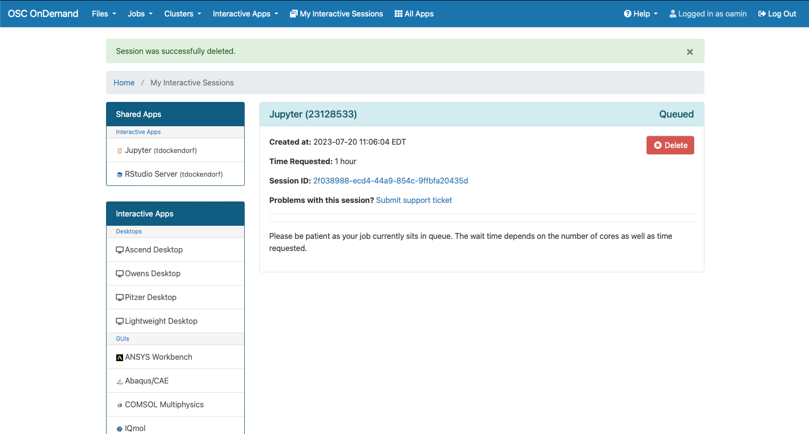
When the job is ready, please click on Connect to Jupyter. This will now launch a Jupyter App.

Jupyter App Usage
With the app open, you will be able to access your home directory on the left and all your available kernels will appear on the right. Any custom kernels created using HOWTO: Use a conda/virtual environment with jupyter will also appear in this selection.
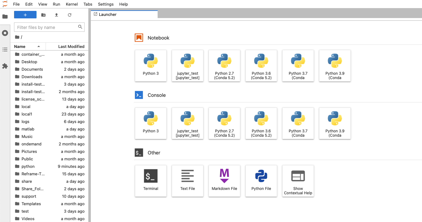
With a file open you can easily switch between different kernels by clicking the kernel name in the top right.
Service:
HOWTO: Use VNC in a batch job
SSHing directly to a compute node at OSC - even if that node has been assigned to you in a current batch job - and starting VNC is an "unsafe" thing to do. When your batch job ends (and the node is assigned to other users), stray processes will be left behind and negatively impact other users. However, it is possible to use VNC on compute nodes safely.
You can use OnDemand, which is a much easier way to access desktops. If your work is not a very large, very intensive computation (for example, you do not expect to saturate all of the cores on a machine for a significant portion of the time you have the application you require open - e.g., you are using the GUI to set up a problem for a longer non-interactive compute job), you can choose one VDI under "Virtual Desktop Interface" from "Desktops" menu. Otherwise, please use "Interactive HPC" from Desktops" menu.
The examples below are for Pitzer. If you use other systems, please see this page for supported versions of TurboVNC on our systems.
Starting your VNC server
Step one is to create your VNC server inside a batch job.
Option 1: Interactive
The preferred method is to start an interactive job, requesting an gpu node, and then once your job starts, you can start the VNC server.
salloc --nodes=1 --ntasks-per-node=40 --gpus-per-node=1 --gres=vis --constraint=40core srun --pty /bin/bash
This command requests an entire GPU node, and tells the batch system you wish to use the GPUs for visualization. This will ensure that the X11 server can access the GPU for acceleration. In this example, I have not specified a duration, which will then default to 1 hour.
module load virtualgl
module load turbovnc
Then start your VNC server. (The first time you run this command, it may ask you for a password - this is to secure your VNC session from unauthorized connections. Set it to whatever password you desire. We recommend a strong password.)
vncserver
To set the vnc password again use the
vncpasswd command.The output of this command is important: it tells you where to point your client to access your desktop. Specifically, we need both the host name (before the :), and the screen (after the :).
New 'X' desktop is p0302.ten.osc.edu:1
Connecting to your VNC server
Because the compute nodes of our clusters are not directly accessible, you must log in to one of the login nodes and allow your VNC client to "tunnel" through SSH to the compute node. The specific method of doing so may vary depending on your client software.
The port assigned to the vncserver will be needed. It is usually 5900 + <display_number>. e.g.
New 'X' desktop is p0302.ten.osc.edu:1
would use port 5901.
Linux/MacOS
Option 1: Manually create an SSH tunnel
I will be providing the basic command line syntax, which works on Linux and MacOS. You would issue this in a new terminal window on your local machine, creating a new connection to Pitzer.
ssh -L <port>:<node_hostname>.ten.osc.edu:<port> <username>@pitzer.osc.edu
The above command establishes a proper ssh connection for the vnc client to use for tunneling to the node.
Open your VNC client, and connect to localhost:<screen_number>, which will tunnel to the correct node on Pitzer.
Option 2: Use your VNC software to tunnel
This example uses Chicken of the VNC, a MacOS VNC client. It is a vncserver started on host n0302 with port 5901 and display 1.
The default window that comes up for Chicken requires the host to connect to, the screen (or port) number, and optionally allows you to specify a host to tunnel through via SSH. This screenshot shows a proper configuration for the output of vncserver shown above. Substitute your host, screen, and username as appropriate.
When you click [Connect], you will be prompted for your HPC password (to establish the tunnel, provided you did not input it into the "password" box on this dialog), and then (if you set one), for your VNC password. If your passwords are correct, the desktop will display in your client.
Windows
This example shows how to create a SSH tunnel through your ssh client. We will be using Putty in this example, but these steps are applicable to most SSH clients.
First, make sure you have x11 forwarding enabled in your SSH client.
Next, open up the port forwarding/tunnels settings and enter the hostname and port you got earlier in the destination field. You will need to add 5900 to the port number when specifiying it here. Some clients may have separate boxes for the desination hostname and port.
For source port, pick a number between 11-99 and add 5900 to it. This number between 11-99 will be the port you connect to in your VNC client.
Make sure to add the forwaded port, and save the changes you've made before exiting the configutations window.
Now start a SSH session to the respective cluster your vncserver is running on. The port forwarding will automatically happen in the background. Closing this SSH session will close the forwarded port; leave the session open as long as you want to use VNC.
Now start a VNC client. TurboVNC has been tested with our systems and is recommended. Enter localhost:[port], replacing [port] with the port between 11-99 you chose earlier.
If you've set up a VNC password you will be prompted for it now. A desktop display should pop up now if everything is configured correctly.
How to Kill a VNC session?
Occasionally you may make a mistake and start a VNC server on a login node or somewhere else you did not want to. In this case it is important to know how to properly kill your VNC server so no processes are left behind.
The command syntax to kill a VNC session is:
vncserver -kill :[screen]
In the example above, screen would be 1.
You need to make sure you are on the same node you spawned the VNC server on when running this command.
Service:
Fields of Science:
HOWTO: Use a Conda/Virtual Environment With Jupyter
The IPython kernel for a Conda/virtual environment must be installed on Jupyter prior to use. This tutorial will walk you though the installation and setup procedure.
First you must create a conda/virtual environment. See create conda/virtual environment if there is not already an environment that has been created.
Install kernel
Load the preferred version of Python or Miniconda3 using the command:
module load python
or
module load miniconda3
Replace "python" or "miniconda3" with the appropriate version, which could be the version you used to create your Conda/venv environment. You can check available Python versions by using the command:
module spider python
Run one of the following commands based on how your Conda/virtual environment was created. Replace "MYENV" with the name of your Conda environment or the path to the environment.
-
If the Conda environment was created via
conda create -n MYENVcommand, use the following command:~support/classroom/tools/create_jupyter_kernel conda MYENV
-
If the Conda environment was created via
conda create -p /path/to/MYENVcommand, use the following command:~support/classroom/tools/create_jupyter_kernel conda /path/to/MYENV
-
If the Python virtual environment was created via
python3 -m venv /path/to/MYENVcommand, use the following command~support/classroom/tools/create_jupyter_kernel venv /path/to/MYENV
-
If you would like to create a kernel for the Python environment iin a container, use the following command
~support/classroom/tools/create_jupyter_kernel container /path/to/container
The resulting kernel name appears as "MYENV [/path/to/MYENV]" in the Jupyter kernel list. You can change the display name by appending a preferred name in the above commands. For example:
~support/classroom/tools/create_jupyter_kernel conda MYENV "My_Research_Project"
This results in the kernel name "My_Research_Project" in the Jupyter kernel list.
You should now be able to access the new Jupyter kernel on OnDemand in a jupyter session. See Usage section of Python page for more details on accessing the Jupyter app.
Install Jupyterlab Debugger kernel
According to Jupyterlab page, debugger requires ipykernel >= 6. Please create your own kernel with conda using the following commands:
module load miniconda
conda create -n jupyterlab-debugger -c conda-forge "ipykernel>=6" xeus-python
~support/classroom/tools/create_jupyter_kernel conda jupyterlab-debugger
You should see a kernelspec 'conda_jupyterlab-debugger' created in home directory. Once the debugger kernel is done, you can use it:
1. go to OnDemand
2. request a JupyterLab app with kernel 3
3. open a notebook with the debugger kernel.
4. you can enable debug mode at upper-right kernel of the notebook
Manually install kernel
If the create_jupyter_kernel script does not work for you, try the following steps to manually install kernel:
# change to the proper version of python
module load python
# replace with the name of conda env
MYENV=useful-project-name
# create the cpnda enironment
conda create -n $MYENV
# Activate your conda/virtual environment
## For Conda environment
source activate $MYENV
# ONLY if you created venv instead of conda env
## For Python Virtual environment
source /path/to/$MYENV/bin/activate
# Install Jupyter kernel
python -m ipykernel install --user --name $MYENV --display-name "Python ($MYENV)"
Remove kernel
If the envirnoment is rebuilt or renamed, users may want to erase any custom jupyter kernel installations.
Be careful! This command will erase entire directories and all files within them.
rm -rf ~/.local/share/jupyter/kernels/${MYENV}
Service:
Fields of Science:
HOWTO: Use an Externally Hosted License
Many software packages require a license. These licenses are usually made available via a license server, which allows software to check out necessary licenses. In this document external refers to a license server that is not hosted inside OSC.
If you have such a software license server set up using a license manager, such as FlexNet, this guide will instruct you on the necessary steps to connect to and use the licenses at OSC.
Users who wish to host their software licenses inside OSC should consult OSC Help.
You are responsible for ensuring you are following your software license terms. Please ensure your terms allow you to use the license at OSC before beginning this process!
Introduction
Broadly speaking, there are two different ways in which the external license server's network may be configured. These differ by whether the license server is directly externally reachable or if it sits behind a private internal network with a port forwarding firewall.
If your license server sits behind a private internal network with a port forwarding firewall you will need to take additional steps to allow the connection from our systems to the license server to be properly routed.
License Server is Directly Externally Reachable
License Server is Behind Port Forwarding Firewall
Unsure?
If you are unsure about which category your situation falls under contact your local IT administrator.
Configure Remote Firewall
OSC changed NAT IP addresses on May 13, 2025. Please update the IP addresses of license server configured for the firewall to allow the connections from nat.osc.edu (192.148.249.249).
In order for connections from OSC to reach the license server, the license server's firewall will need to be configured. All outbound network traffic from all of OSC's compute nodes are routed through a network address translation host (NAT).
The license server should be configured to allow connections from nat.osc.edu including the following IP addresses to the SERVER:PORT where the license server is running:
- 192.148.249.249
A typical FlexNet-based license server uses two ports: one is server port and the other is daemon port, and the firewall should be configured for the both ports. A typical license file looks, for example,
SERVER licXXX.osc.edu 0050XXXXX5C 28000
VENDOR {license name} port=28001
In this example, "28000" is the server port, and "28001" is the daemon port. The daemon port is not mandatory if you use it on a local network, however it becomes necessary if you want to use it outside of your local network. So, please make sure you declared the daemon port in the license file and configured the firewall for the port.
Confirm Configuration
The firewall settings should be verified by attempting to connect to the license server from the compute environment using telenet.
Get on to a compute node by requesting a short, small, interactive job and test the connection using telenet:
telnet <License Server IP Address> <Port#>
(Recommended) Restrict Access to IPs/Usernames
It is also recommended to restrict accessibility using the remote license server's access control mechanisms, such as limiting access to particular usernames in the options.dat file used with FlexNet-based license servers.
For FlexNet tools, you can add the following line to your options.dat file, one for each user.
INCLUDEALL USER <OSC username>
If you have a large number of users to give access to you may want to define a group using GROUP within the options.dat file and give access to that whole group using INCLUDEALL GROUP <group name> .
Users who use other license managers should consult the license manager's documentation.
Modify Job Environment to Point at License Server
The software must now be told to contact the license server for it's licenses. The exact method of doing so can vary between each software package, but most use an environment variable that specifies the license server IP address and port number to use.
For example LS DYNA uses the environment variable LSTC_LICENSE and LSTC_LICENSE_SERVER to know where to look for the license. The following lines would be added to a job script to tell LS-DYNA to use licenses from port 2345 on server 1.2.3.4, if you use bash:
export LSTC_LICENSE=network export LSTC_LICENSE_SERVER=2345@1.2.3.4
or, if you use csh:
setenv LSTC_LICENSE network setenv LSTC_LICENSE_SERVER 2345@1.2.3.4
License Server is Behind Port Forwarding Firewall
If the license server is behind a port forwarding firewall, and has a different IP address from the IP address of the firewall, additional steps must be taken to allow connections to be properly routed within the license server's internal network.
- Use the license server's fully qualified domain name in SERVER line in the license file instead of the IP address.
- Contact your IT team to have the firewall IP address mapped to the fully qualified domain name.
Software Specific Details
The following outlines details particular to a specific software package.
ANSYS
Uses the following environment variables:
ANSYSLI_SERVERS=<port>@<IP> ANSYSLMD_LICENSE_FILE=<port>@<IP>
If your license server is behind a port forwarding firewall and you cannot use a fully qualified domain name in the license file, you can add ANSYSLI_EXTERNAL_IP={external IP address} to ansyslmd.ini on the license server.
HOWTO: Use ulimit command to set soft limits
This document shows you how to set soft limits using the ulimit command.
The ulimit command sets or reports user process resource limits. The default limits are defined and applied when a new user is added to the system. Limits are categorized as either soft or hard. With the ulimit command, you can change your soft limits for the current shell environment, up to the maximum set by the hard limits. You must have root user authority to change resource hard limits.
Syntax
ulimit [-HSTabcdefilmnpqrstuvx [Limit]]
| flags | description |
|---|---|
| -H | Specifies that the hard limit for the given resource is set. If you have root user authority, you can increase the hard limit. Anyone can decrease it |
| -S | Specifies that the soft limit for the given resource is set. A soft limit can be increased up to the value of the hard limit. If neither the -H nor -S flags are specified, the limit applies to both |
| -a | Lists all of the current resource limits |
| -b | The maximum socket buffer size |
| -c | The maximum size of core files created |
| -d | The maximum size of a process's data segment |
| -e | The maximum scheduling priority ("nice") |
| -f | The maximum size of files written by the shell and its children |
| -i | The maximum number of pending signals |
| -l | The maximum size that may be locked into memory |
| -m | The maximum resident set size (many systems do not honor this limit) |
| -n | The maximum number of open file descriptors (most systems do not allow this value to be set) |
| -p | The pipe size in 512-byte blocks (this may not be set) |
| -q | The maximum number of bytes in POSIX message queues |
| -r | The maximum real-time scheduling priority |
| -s | The maximum stack size |
| -t | The maximum amount of cpu time in seconds |
| -u | The maximum number of processes available to a single user |
| -v | The maximum amount of virtual memory available to the shell and, on some systems, to its children |
| -x | The maximum number of file locks |
| -T | The maximum number of threads |
The limit for a specified resource is set when the Limit parameter is specified. The value of the Limit parameter can be a number in the unit specified with each resource, or the value "unlimited." For example, to set the file size limit to 51,200 bytes, use:
ulimit -f 100
To set the size of core dumps to unlimited, use:
ulimit –c unlimited
How to change ulimit for a MPI program
The ulimit command affects the current shell environment. When a MPI program is started, it does not spawn in the current shell. You have to use srun to start a wrapper script that sets the limit if you want to set the limit for each process. Below is how you set the limit for each shell (We use ulimit –c unlimited to allow unlimited core dumps, as an example):
- Prepare your batch job script named "myjob" as below (Here, we request a job with 5-hour 2-cores):
#!/bin/bash #SBATCH --ntasks=2 #SBATCH --time=5:00:00 #SBATCH ... ... srun ./test1 ...
- Prepare the wrapper script named "test1" as below:
#!/bin/bash ulimit –c unlimited .....(your own program)
-
sbatch myjob
Service:
HOWTO: Using MLFlow to track ML training and models
MLflow is a tool for managing the training and deployment of machine learning models.
At OSC, MLflow is available to help researchers and developers efficiently track training runs and manage models when working. This guide explains how to access MLflow at OSC, run example notebooks, and visualize your experiment data using the MLflow UI. MLflow is available on OSC clusters as part of the PyTorch module or can be installed to your virtual environment via package managers such as pip, conda, or uv.
We provide a repository with marimo notebooks demonstrating how to integrate MLflow into your training and inference codes on UCR.
To run them at OSC:
- Clone the repository
- Select the marimo OnDemand app from the list of apps.
- In the field labeled
Working Directory or Notebook, specify the path to one of the notebooks in the repo. - Select the
Sandbox environmentcheckbox. - The first time you run a notebook in sandbox mode, you may be asked to install missing package dependencies. After the packages have been installed, restart the kernel or start a new marimo ondemand job.
Running the code in the notebooks will create an mlruns/ subdirectory in your local copy of the repository, which contains all of the logged training run data and any registered models. As described in the notebooks, this tracking data can be accessed via Python API. It is also possible to use the MLflow UI, which is available via the MLflow OnDemand app, to graphically view the data collected while executing the notebook. To view the data generated by these notebooks, set the Tracking URI directory to your local copy of the respository.
For more information about how to use MLflow read their documentation.
Note that MLflow offers several options for deploying MLflow servers as described in the MLflow docs. No servers have been deployed at OSC, but if this is necessary for your research please submit a ticket.
HOWTO: test data transfer speed
The data transfer speed between OSC and another network can be tested.
Test data transfer speed with iperf3 tool
Connect to a data mover host at osc and note the hostname.
$ ssh sftp.osc.edu # login $ hostname gcs01.hpc.osc.edu # the hostname may also be gcs02.hpc.osc.edu
From there, an iperf3 server process can be started. Note the port used.
iperf3 -s -p 5201 Server listening on 5201 # the above port number could be different
Test Upload Performance
Next, on your local machine, try to connect to the iperf3 server process
iperf3 -c gcs01.hpc.osc.edu -p 5201
If it connects sucessfully, then it will start testing and then finish with a summary
Connecting to host gcs01.hpc.osc.edu, port 5201 ... - - - - - - - - - - - - - - - - - - - - - - - - - [ ID] Interval Transfer Bitrate [ 7] 0.00-10.00 sec 13.8 MBytes 11.6 Mbits/sec sender [ 7] 0.00-10.00 sec 13.8 MBytes 11.6 Mbits/sec receiver
Test Download Performance
For the data downloaded speed, you can also test the newwork performace in the reverse direction, with the server on gcs01 sending data, and the client on your computer receiving data:
iperf3 -c gcs01.hpc.osc.edu -p 5201 -R
Run iperf3 using docker (alternative)
Docker can be used if iperf3 is not installed on client machine, but docker is.
$ docker run --rm -it networkstatic/iperf3 -c gcs01.hpc.osc.edu -p 5201
Make sure iperf3 server process is running on OSC GCS host or client iperf3 will fail with error.
Citation
The Ohio Supercomputer Center provides High Performance Computing resources and expertise to academic researchers across the State of Ohio. Any paper citing this document has utilized OSC to conduct research on our production services. OSC is a member of the Ohio Technology Consortium, a division of the Ohio Department of Higher Education.
Hardware
OSC services can be cited by visiting the documentation for the service in question and finding the "Citation" page (located in the menu to the side).
HPC systems currently in production use can be found here: https://www.osc.edu/supercomputing/hpc
Decommissioned HPC systems can be found here: https://www.osc.edu/supercomputing/hpc/decommissioned.
Logos
Please refer to our branding webpage.
Citing OSC
We prefer that you cite OSC when using our services, using the following information, taking into account the appropriate citation style guidelines.
Ohio Supercomputer Center. 1987. Ohio Supercomputer Center. Columbus OH: Ohio Supercomputer Center. https://ror.org/01apna436.
BibTeX:
@MISC{Ohio_Supercomputer_Center1987-dl,
title = "Ohio Supercomputer Center",
author = "{Ohio Supercomputer Center}",
publisher = "Ohio Supercomputer Center",
year = "1987",
url = "https://ror.org/01apna436"
}
ris:
TY - MISC AU - Ohio Supercomputer Center TI - Ohio Supercomputer Center PY - 1987 DA - 1987 PB - Ohio Supercomputer Center UR - https://ror.org/01apna436
New User Training
Transcript:
Kate Cahill
[Slide: “An Introduction to OSC Resources and Services”]
All right, so thank you again for everyone for joining and we'll get started. So today I'm going to give you an introduction to OSC resources and services. So, talking about our systems, and how you can get to use them as a researcher.
[Slide: “Kate Cahill Education & Training Specialist”]
As I said, my name is Kate and I do education and training for OSC.
[Slide: “Outline”]
So today we're going to cover just general, you know, intro to OSC Intro to high performance, computing so some concepts and definitions that are useful to know if you're new to using HPC systems. I'll talk about the hardware that we have at OSC, and then some details on how to get a new account or a new project, if you're starting a new research project with us. We'll take a short break, and then the latter part of the presentation will be about using the system. So, the user environment, how to work with software on the clusters and an intro to batch processing and running jobs on the systems. And then we'll finish. I'll just do a demonstration of our OnDemand web portal, so you can see what that looks like if you haven't logged into it already, and I’ll highlight the features of that, and how that makes it easy to get started. So like I said, you can put questions in the chat. Let me know if you can't hear me, or if something's not clear, and you can also ask questions as we go. I'll pause between our sections.
[Slide: “What is the Ohio Supercomputer Center?”]
So what is the Ohio supercomputer center?
[Slide: “About OSC”]
We are a part of the Ohio Department of Higher Education and we’re part of a group that's called OH-TECH, which is a statewide consortium for technology support services. So OH-TECH is comprised of OSC, OhioLINK, which is the digital library services, and OARnet, which is the the statewide network system that we have. And so, we are a statewide resource for all higher education institutions in Ohio, and we provide, you know, different types of high performance computing services and computational science expertise. And we, you know, are meant to serve the whole State.
[Slide: “Service Catalog”]
So here is some details about the services that we have at OSC. So I’m sure you’re aware that we have, you know, HPC clusters. So, that's the main reason people come to OSC is to use our large-scale computing resources. But we also have other services, such as data storage for different research needs, education activities. So you know, training events like this one, you know we can do training, you know, at your institution or for your department or group. We also partner with people on education projects to use HPC in classes and develop curriculum for computational science of different kinds. And we do a lot of web software development. So we have a team that's focused on developing different types of software and tools to use HPC resources on the web. And that's where we get our OnDemand portal. So that's their main focus. And then scientific software development as well. So, we manage the software that we have on our clusters. But we also partner with people to develop new software optimize existing things to make software run better on HPC systems.
[Slide: “Client Services”]
So, here's just an overview of kind of the activities that OSC was involved in, and this is fiscal year, 22. So this is the end of 2021, and the first half of 2022. So we had 55 active Ohio universities, with projects, 68, Ohio, or 68 companies or industry, part, you know people that were active doing research on our systems, 54 nonprofits and government agencies had active users and then we had other educational institutions with active accounts at OSC. And we have almost 8,500 active clients at this point, so people with accounts who are using our systems. And a 1,000 of those a little more than a 1,000 of those are PIs, so those are people that that run projects and lead research. And you can see the breakdown of roles, you know, for the people that we have accounts for. So about a quarter of them or faculty or staff, and the bulk of them are students. And we had a 127 college courses that used OSC so we have classroom projects that are separate from our research projects, and you can, you know, use those to have your students access OSC and do course work and homework for your courses. Twenty-nine training opportunities such as this one with the over 700 trainees.
[Slide: “HPC Concepts”]
And so that's just a general overview of OSC. Let me know if you have any questions about what we do or any of our services. But now I want to talk about HPC concepts. So, a lot of people who use OSC are new to HPC in general. So I’m just going to talk with generally about some concepts and define some terms.
[Slide: “Why Use HPC?”]
So, there's a lot of reasons why people need to use high performance computing resources. You know, typically people have some analysis or simulation that they want to run, that, you know, if they want to run it at a larger scale, it's just going to take days or weeks on a typical desktop computer. And so, they just need more computing power, so more cores, more ability to parallelize other types of acceleration, like using GPUs, or just using distributed computing tools like Spark. Or it may be that you're working with data sets, or you're collecting data, and it's just a very large volume of data, and it's really hard to work with that, you know, given the storage, or the memory that you have on your own systems. So, we have large memory nodes for that purpose. And then you know, more storage in general so you can work with larger data sets. Or it could be that there's a particular software package that just works best on HPC systems, and you can't access it otherwise.
[Slide: “What is the difference between your laptop and a supercomputer?”]
So here are three general points that it's good to keep in mind about what's the difference between your laptop or desktop and a supercomputer. So one way to think about a supercomputer is thinking about you know thousands or tens of thousands of individual computers that are linked together through a high, a very high-speed network, and so that you know, so you can, you know, link them all together so they can work together to do larger scale computing. That's really how we get the supercomputers. Another thing to keep in mind is that nobody is going to the computer itself. No one is standing in front of the supercomputer and working with it directly through a you know, a monitor and a keyboard. Everybody is remotely connecting to these systems. So they're all you know in in a in a separate, a separate area, you know, and we're all logging into them remotely. And so it's just important to keep in mind that your activity on the system is kind of moderated by the network that you're using. So if you're on a fast network, you know, you're going to get really good integration with what you're doing and really good response rates. If you're on a slower network, if you're, you know, somewhere with a slow wi-fi connection, you're going to see a slower response. So just keep that in mind when you're working with the systems. And then the third point is that these systems are shared. So you saw that, I said we have over almost 8,500 clients active on our systems this past year, and so at any given time hundreds of people are logged on and using the system or running jobs. So there's just some things that we ask you to do, so that we can all use the system, and everyone can have their jobs completed and their research move forward as efficiently as possible. So there's certain things that that the system we have, the system set up in a certain way, so that it can be shared effectively.
[Slide: “HPC Terminology”]
So here's some terminology that's good to know for using HPC systems. So we talk a lot about a node or a compute node. And so a node is sort of the unit of a cluster, and it's it's kind of equivalent to a high end desktop. It has its own memory, it has its own storage, it has its own processors. And so you know, each of those nodes is sort of like a desktop computer, and then they're all linked together, and they create the cluster. And so the compute cluster is that group of nodes that are connected by a high-speed network, and that forms the supercomputer. So, a supercomputer and a cluster, or a about synonymous. And a core we often talk about a core that usually is, relates to a processor or a CPU, and so you'll see I'll explain our hardware in a minute, and I’ll talk about cores per node. So that's really processors CPUs per node. And so, there's usually multiple cores per processor, chip and per node. And so you need to know that architecture when you make a request to the system. And then, finally, we refer a lot to GPUs, and those are graphical processing units. So, this is a separate type of processor that does much more kind of very parallel work. We refer to it often as an accelerator because it it's really good at doing some, you know, a lot of small calculations really, quickly, and so depending on the type of work you have to do, if it can be broken up effectively to use a GPU, it can speed up your work a lot. So GPUs have become very popular in lots of different workflows. So they're a big part of super computers now.
[Slide: “Memory”]
And some of the things to keep in mind memory is the really fast storage that holds the data that is being calculated on. So in an active an active job or simulation or analysis, memory is holding the data that's being used for that analysis. And so in a supercomputer we have memory, that is, you can have shared memory, some memory that's shared across all of your processors on a single node. The memory will be shared for all the processors on that node. If you use more than one node in your calculations then you're going to have distributed memory where the know the memory on one node won't be the same as the memory on the on another node, and you have to make sure that your calculation has all the information it needs. So, there's different types of decisions you have to make about how to use the system to, you know, speed up your code as much as much as possible, taking into account the different memory that's available to you. And each core has an associated amount of memory. So, we don't require that you tell us how much memory you need you just make a node and core request, and then we give you a relative amount of memory associated with that number, of course. But I'll go into more detail with the hardware.
[Slide: “Storage”]
And for storage. So, storage is where you're, you're keeping things for a longer term. Then you would keep you keep data in memory. And so you can have storage that is, you know, active in a in an active job holding, you know, data that's already been created, or it's already been analyzed. And you just need that for your output. And then there's longer term storage, for you know different purposes as well, and I’ll go over our data storage options at OSC.
[Slide: “Structure of a Supercomputer”]
And so here is just a way to look at the supercomputer kind of covering all these concepts. So you can see the compute nodes are labeled at the bottom, and so those are the individual nodes that are network together to form the cluster. So that's the main part of the supercomputer. We have a separate type of node called the login node. That's for just kind of setting up jobs and reviewing output, but not for your main compute. And then you, as the researcher, are accessing this through some kind of network, either using a terminal program or a web portal. And then every and then the data storage options are available, you know, to access through the login nodes and the compute nodes as well.
[Slide: “Hardware Overview”]
So, any questions about general HPC things or General OSC surfaces. So, I'll go on to talk about the hardware that we have at OSC.
[Slide: “System Status”]
So at this point, so right now we have three systems that are currently active, and that's Owens, Pitzer and Ascend, and Pitzer is really divided into two sections. The original Pitzer and Pitzer expansion. So that's what you see here. So, Owens has been around the longest, Ascend just came online at the end of last year. And so, the larger systems are Owens and Pitzer. You can see if you look at the node, count that Ascend is a lot smaller. It's more specialized. So, it's a GPU focused system. So, unless you have work that is really GPU heavy that you need, GPUs, you may not, and you may not Ascend at all. Owens and Pitzer are still our main systems. And then, so yeah, that kind of gives you the general sense of the systems. But now I’m going to talk more specifically about each of them.
[Slide: “Owens Compute Nodes”]
So on Owens, Owens has 648 standard nodes. Those are standard compute nodes, and each of those has 28 cores or processors per node, and 128 GB of memory. So that's a standard compute node on Owens
[Slide: “Owens Data Analytics Nodes”]
Owens also has 16 large memory nodes. Each of those nodes has 48 cores per node and one and a half terabytes of memory, as well as 12 TB of local disk, space or storage. And so those are, for you know the types of jobs that need just a lot of memory to, you know hold all the data that's being, you know, calculated, or to do all the analytics that needs to be done.
[Slide: “Owens GPU Nodes”]
And Owens also, in addition to the regular compute nodes, has a 160 GPU nodes. And so, these are the same as the standard compute nodes so 28 cores per node, but they also have one NVIDIA P100 GPUs on them. So, each node has one GPU.
[Slide: “Owens Cluster Specifications”]
And so here is kind of all those parts of Owens put together. And this may be hard to read. It's not very large. But you can definitely look at all of these details and more specifications on Owens on our main website. If you just go under cluster computing, and you can choose Owens. You can see all these details.
[Slide: “Pitzer Cluster Specifications Original”]
And so here is the overview for Pitzer. So this is the original part of Pitzer. And so this has 224 standard nodes, with 40 cores per node. And 192 GB of memory, and a terabyte of local storage per node. There's also 32 GPU nodes on Pitzer with the same 40 cores per node.
There's more memory, and there's two GPUs per node on Pitzer. So it's depending on the workload you need to you need to run. You might need, you know, two GPUs per note instead of one. And then there are four huge memory notes on Pitzer as well. Those are 80 cores per node and 3 TB of memory. So again, you know, these are for jobs that need a lot of single node parallelization. So you can use a lot of cores on one node, and you need a lot of memory.
[Slide: “Pitzer Cluster Specifications”]
Here we go, and so Pitzer, so the expansion of Pitzer, in addition to the original Pitzer, the expansion has 340 standard nodes, and those each have 48 cores per node. And then 42 GPU nodes as well. And again, those are two GPUs per node. And there's also 12 large memory nodes on the Pitzer expansion as well. And for dense GPU nodes so for jobs that that can take advantage of, for you can use four GPUs per node we have a couple of nodes for that as well. And again, the details of this are on our website. That's where you can see all of the technical specifications for our clusters.
[Slide: “Ascend Cluster Specifications”]
And so Ascend like I said, it's the newest system. It's much smaller in in sort of node counts than Owens or Pitzer and so it's mainly focused on GPU nodes. So Ascend has 24 GPU nodes, with 88 total cores per node and 4 GPUs per node as well. So yeah, like, I said, this is GPU focused system. So, if your if your work is going to be, you know, very GPU heavy you can request access to the system, but we didn't give general access to everyone because it's not very large, and it's kind of specialized.
[Slide: “Login Nodes - Usage”]
And just to reiterate the login nodes. So, each of the systems has login nodes, and so that's when you first log into the system you're on the login nodes. And so, this is where you will set up your files, edit files, you know, get your input data and everything together to submit a job to the batch system so that you can access the compute nodes. This is not where you're going to run your jobs. There's very small limits on the login nodes as to how long any process can run, so if you start a process of some kind, it'll get stopped after 20 min. And you only have access to 1 GB of memory on the login nodes. So, they're really not for compute that you can do some small scale work, you know, like opening a graphical interface, or compiling like a very small code as long as it's really, you know not very compute intensive and won't take very long. But you don't want to use it too much, because it can slow down the login notes for everybody else. So the login nodes are mainly for setting up your jobs and looking at output, not for actually computing. And that's why we want you to use the batch system to use the compute nodes.
[Slide: “Data Storage Systems”]
So now I’m going to talk about our data storage systems. Any questions?
[Slide: “File Systems at OSC”]
So we have several file systems that OSC for different purposes. I'm going to talk about four of them. So, you can see them here on the data storage on the left. We have the home file system, the project file system, the scratch file system, and then the compute nodes. So, the storage that's available on the compute nodes. Those are the ones that I’m going to focus on.
[Slide: “Research Data Storage”]
And so the some of the features of these different file systems, the home location. So every account, so if you have an account at OSC, you'll have a location that that's your home directory, and that'll be on the home file system. And most accounts will have 500 GB storage available in the home directory. There might be some accounts that that have less, but almost all of them will have the 500 GB, and this is the main place that we expect that you can use to store your files, and we back this up regularly. So if you happen to lose something, or accidentally delete something vital, you can let us know, and we can help you restore it. So, we consider this kind of permanent protected storage. And then but if your group or your project needs more storage, then is available in each of the user accounts, then the project PI can request access to the project file system. And so this is just like a supplemental storage to the home directories. Most PIs or most groups need about one to 5 TB of storage on the project file system, and it's accessible to everybody in that project. And then there's also the scratch file system available. And this is available to everyone, you don't have to request access, so you can access it directly, and this is, we consider temporary storage. So we don't back up the scratch file system so you can use it, for you know large files that you might not want to fill your home directory up with. You can put them there if you're going to be actively using them, for you know, a couple of weeks or months, and you just want to keep them, you know, somewhere else than your Home Directory. That's what the scratch file system is for. And then on the compute nodes each compute node that you'll have access to will have its own storage. And so it's for use during your job. And so ideally, all of your compute. And you know, file creation, file, generation output, creation will happen on the compute node, and then at the end of the job you'll just copy everything back to your home directory. So you're not, you know, using the network to during your job to read and write. It just makes your job more efficient kind of reduces the overhead of that of that network usage, but you only have access to it while your job is running. So at the end of the job, you all that information is removed. So you said to make sure to copy back your results at the end of your job. We also have archive storage. So if you have some data set or database that you want to have, you know, stored for a longer period of time. They're not going to access regularly. You can talk to us. You can email OSC help and ask about that as well.
[Screen: Table showing Filesystem, Quota, Network, Backed-Up?, Purged]
And so here's just kind of an overview of the different features of the file systems. So, and I've included on the on the left. So the name of the file, the file system is home. You can use the variable dollar sign home as a reference to your home directory for the project file system. It's FSESS or FS Project, I think it's just FSESS. And then your project code to reach your project files. If you have that as a separate request the scratch file system you can reach by FS scratch, and then your project code, and then you can reference the location of the compute. Compute node storage with the TMPDIR and you can see the quotas so generally the quota for the home directory is a half terabyte. The project file system is you know amount that you choose. That's by request. We have a nominal quota of a 100 TB on the scratch file system and the compute. The compute file system varies, but it's usually at least 1 TB per node. You can see the different network speeds for the file system. So like I said, the home and the project or not very fast, the scratch file system has a faster network. So that is, you know, if you wanted to keep a large data set on the scratch file system and use it during a job. The scratch file system is more optimized for that. The home and project are backed up, scratch and compute are not. And we do have a purge on the scratch file system about every 90 days, so that is, if you have some files out there that you haven't used in a while, you know if they're you know. If they get old, they haven’t been they haven't been access for 90 days, they might be purged. We don't always purge, but when it gets full, we do, and then the compute node file system is removed when your job ends, so you only have access to it while your job is running. And again, there's links here on the bottom about where you can get more details about the file systems.
[Slide: “Getting Started at OSC”]
And I see information question in the chat. But sounds like you got the information you needed. So any other question, any questions about file systems or hardware?
Olamide E Opadokun:
Yeah. So the other file types that are backed up, for how long are they kept on the system?
Kate Cahill:
So you mean, like in the Home Directory?
Olamide E Opadokun:
Yeah.
Kate Cahill:
So there's a couple of layers to that. So Wilbur, do you know what our current scheme is for that? I know we back it up like multiple times a day, but then we have offsite backups as well. So I think it might be up to two weeks, or maybe further.
Wilbur Ouma:
Yeah, I don't have the correct, all the information on that. Yeah. But I know we do back up almost several times per day. Yeah, but we've had some requests people coming back that maybe they inadvertently deleted some files or data, maybe the last, you know a month or several weeks, and we've been able to recover those.
Kate Cahill:
Yeah, so I would certainly say that if you, if you do find that something has been deleted that you want recovered to let us know as soon as possible, because, you know, we don't keep them, you know, for months back, or anything. So you don't want it to wait too long. But at least couple of weeks, I believe.
Olamide E Opadokun:
Okay. So they kept on the system for a couple of weeks and then deleted?
Kate Cahill:
So the backups. So it's, you know we take. We take backups of the home directories, and we can restore things that have been deleted from a from an earlier version. And then we have offsite backups as well. So if we, if we happen to have some problem with our system and we lose power, we have versions that are stored off site as well. It's just a question of kind of like, how long those like you how far back those backups go. But yeah, so it's more about, you know. If you if you remove something and then you want it back, we can restore an earlier version of it. Once you let us know that you need it again. But on the home directory and the project directory we don't remove anything, so it's entirely up to you what's on those.
Olamide E Opadokun:
Oh, okay, so that that's not what subjected to the long-term storage, the archive storage, because that's just always going to be available right?
Kate Cahill:
Yeah. So the archive storage is a separate storage. So it's not like we automatically archive your home directory. That would be, you’d have to ask us to put something on the archive storage. It would be separate.
Olamide E Opadokun:
Okay, thank you.
Michael Broe:
So the issue, I often I advise graduate students who are working with PIs, who have. So the PI has the OSC account, and then they move away. They go to different jobs that if they go. And so then they ask me, can I get access to my data again? And I'm just would like to clarify if the PI doesn't keep this under control. How long will the data hang around, or how can they access it. If and so they've moved on from the OSU. And so, they no longer have an OSU account and they're trying to get access to data from, maybe several years ago, because their papers just been published. I know it's a big issue, a difficult issue. But I just like to clarify what is going on there.
Kate Cahill:
Yeah. So when someone leaves OSU and is no longer active their account. So I mean, if like, if they're not, if they're not part of your group anymore, and you're not working with them. And you don't, you know you're not going to have them on your OSC account. You know their OSC account will kind of just sort of age. It doesn't get automatically removed, but it goes into a restricted state, and then it goes into an archive state, and we remove that home directory. So it's always a good idea when somebody is leaving, so like, you know, for the PI to make a backup of that of that students' information at OSC so they have access to it if they need something from an earlier project. But yeah, certainly, after a couple of years, and I don't think that we could, that we would still have the student’s home directory data available unless there was some, you know, archive process that we actually said, “Put this on an archive.” I think from our perspective it's up to the PI, the person that runs the project to, you know, make a backup of that information. So, they have it like, make it back up way from OSC.
Michael Broe:
Yeah, or the if they believe the project is going to continue it, it's on the project. It's going to be backed up in, as long as the project exists.
Kate Cahill:
Right, so, if so, yeah, if the student has data in their home directory that everybody else wants to have access to for the project to continue, they should move it to the project directory. That's the shared space between all of the accounts that will stay as long as long as the OSC, the overall project is still there. So, if you have that project that shared project space for everybody in your in your group. You can, you can use that as another way to keep that that information available to everybody else. But yeah, it's definitely something that has to be kind of, there has to be a procedure when somebody leaves to make sure that that data isn't lost.
Michael Broe:
Yes, great, that's the perfect answer. Thank you.
Kate Cahill:
Alright great, so I’m going to start to talk about how to get started at OSC. So, this is more about getting an account and getting a project, and how we manage those things here.
[Slide: “Who can get an OSC Project?”]
So we have different types of projects that are available. So our main type of project is the academic project. And so that's generally led by a PI, and that person is generally a full-time faculty, member or research scientist at an Ohio academic institution. They could also. That's the main type of PI that we have at OSC for academic projects. And so the PI can request a project, and once they have that project, they can put anybody on it that they want, so they can authorize accounts for, you know, students post docs, other faculty, other their staff collectors, people from out of state people from out of the country. Anybody can have an account. But the PI has to have a certain role at an Ohio institution. Another type of project that we have is the classroom project, and so those are for specific courses. So, they're shorter-term projects that are kind of you know, specialized for giving students in a class access to OSC. We also have commercial projects available as well, so commercial organizations can purchase time at OSC as well.
[Slide: “Accounts and Projects at OSC”]
So a project we define a project code. So when you request a new project we'll define a code it becomes with a P, usually has three letters and four numbers, and that is like, I said, headed by a PI and includes any number of other users that the PI authorizes. And this is, and the project is the is how we account for computing resources. An account is a specific user so that will have a specific username and password. And that's how that that person will access OSC systems and the HPC systems. And so, an account is one person. So every person should have a unique account. You can work on more than one project, but you'll just have the one account to access all of them.
[Slide: “Usage Charges”]
And so we do charge for usage of our systems, and those charges are in terms of core hours, GPU hours, and terabyte months. And so, a project will have a dollar balance and any services that you use like compute and storage are charged to that balance and you know we are still subsidized by the state, so our charges are still partially subsidized, and so they're cheaper than your, you know commercial cloud resources. You can see more details on the link here. And yeah. So, if you're interested in in sort of the charges, the specific charges.
[Slide: “Ohio Academic Projects”]
So for academic projects annually, each project can receive a $1,000 grant so that can be your budget for the year, and so that that rolls over every fiscal year. So it'll be the beginning of July. You know, all academic projects will be eligible for a new $1,000 grant and so that's a way to kind of, you know, have a starting budget, and you know, get to use OSC resources, fully subsidized. If you think you're going to need more than that, then you have to add money to that budget. And so we do it this way, so that there are no unexpected charges. So you don't have some, you know, jobs that are over running, you know, or you know that somebody submits too many jobs or they're too big, and they end up charging more. The budget is a hard limit, and we also don't do proposal submissions anymore. We used to have an Allocations Committee that would review proposals, but we don't have that now, since we have this this fee model. The classroom projects that I mentioned before are fully subsidized, so they will have a budget as well. But it is not a budget that will be charged to anyone. And all of these the projects and getting an account are all available at our client portal site which is my.osc.edu.
[Slide: “Client Portal- my.osc.edu”]
And so the client portal, like I said, is mainly for project, management and account management. It's really useful for PIs to kind of oversee the projects, the activity on their projects, so you can. When you log into the client portal. If you're on a project, you'll see some statement about the usage on your projects. So, you can see it broken down by project, by type and system, by usage per day, and then below you'll see your active projects, and then you'll see your budget balance and your usage. So, it's just a way to see that information at a glance, and then you can, you know using the client portal, you can create an account. Keep your email and your password updated. Recover access to your account, if it's restricted, change your shell if you don't want to use the standard batch shell you can change to a different shell, and then you can do things like, manage your users, and request services and resources like storage and software.
[Slide: “Statewide Users Group (SUG)”]
And so OSC, you know, has a statewide users group. So that's you know everybody that uses OSC to give you a chance to provide advice to OSC. So we can hear from the OSC community about. You know what they would like to see OSC do in future kind of where you want to see us go as far as resources or services. So this this group meets twice a year, and there's a chairperson elected yearly from the you know, Ohio Academic community generally, and we have some standing committees that meet as part of this group. So there's Software and Activities Committee and the Hardware and Operations Committee. And this is usually a day long sort of symposium that happens at OSC. But it's also a hybrid event where you can also share your research in poster sessions and Flash talks and meet other OSC researchers. And this happens twice a year, generally April and October. And you can check the OSC calendar to find out information about the next one, which is on April 20th. You can register, you know, present a poster send a flash talk, or just, you know, come and meet OSC staff and other researchers.
[Slide: “Communications & Citing OSC”]
So as far as communications we do send regular user emails, information about downtimes and any other unplanned maintenance events. We do have quarterly downtimes. We just had a downtime yesterday, so we're good for a quarter now. But we want to keep you updated. So make sure your email is is correct so you can receive those. And there's also information on our main website about citation. So if you are gone publish any work you've done with OSC resources, you can. You can cite the resource that you use
[Slide: “Short Break”]
All right, so we're going to take just like a five min break right here, so everybody can get up and move around a little bit, and we'll be back at 1:50. But does anybody have any questions? All right so I’ll be back in five minutes.
[Slide: “Short Break” beginning at about 41:35]
All right, so I’m going to get started again. Does anybody have any questions?
[Slide: “User Environment”]
So now we're going to talk about what it's like to use the systems and some information about HPC systems and software batch system environment.
[Slide: “Linux Operating System”]
So the user environment we use. We have a Linux operating system which is the most widely used in HPC so that's really common. If you have use HPC systems before you've probably interacted with the Linux system. It generally has been a command line based. So you need to have, you know some sense of the commands that you need to enter, to do things like, you know, refiles or move files. There is a choice of shells I mentioned. So bash is the default shell. But there are other shells available. If you you know, want to work at a different shell, you have to change your shell in the client portal. And so then you'll have that environment. And this is open-source software and there's a lot of tutorials available online. We have a couple linked here under the command-line fundamentals page on our website, just as suggestions potential tutorials. It's good to have some command line, comfort like. Just know a couple of standard commands to navigate the file system, for example. Just so you're comfortable in it, but you don't necessarily need to use the command line for most of your work anymore.
[Slide: “Connecting to an OSC Cluster”]
So to connect to an OSC cluster you have a couple of options like I said, everybody connects over a network. So you're going to use some kind of, you know. But you know, network connection tool. The historical way to connect to a system is using ssh through a terminal window. So in a Mac or Linux system you'd open the terminal program, and at the prompt enter ssh and then your user ID and @. And then the name of the sort of address of the system that you want to access. So you could access Owens it'd be owens.osc.edu and SSH. Is the command for secure shell. So you're connecting, you know, to the system through a secure shell. If you have a windows system, I believe there's a terminal program on there now, or you can download some free versions like putty is a terminal program you could use other options for connecting. So the main way that most of OSC clients, the connections, clusters these days is our on Demand portal. So that's our web portal. So you just need a you know you have a browser, and you just need to go to ondemand.osc.edu and enter your OSC user name and password, and then you have access to all the compute resources at OSC. Through the through the browser.
[Slide: “Transferring Files to and from the Cluster”]
Another key step you generally have to take with transferring files. You know you have to take in your set up. Your research is to transfer files to and from the cluster. And so again, you have several options with the command Line tools. You can use sftp or scp, you know, in a terminal window. And so you would, you know. copy either from your local system to the cluster or the other way for smaller files. You can do that right through the login nodes so same kind of connection as the ssh, you can do owens.osc.edu. If your network is slow or your files are larger. You have another option called the file transfer server. So, instead of connecting to Owens or Pitzer directly, you would connect to sftp.osc.edu, and that just gives you access to the same file systems. But you're over a file transfer network that gives you a longer time to transfer file, so there's no time out on there. And so that helps with large files for slow networks. On the OnDemand portal. We have file management tools that include file transfer tools, so you can do a drag and drop to transfer files or use the upload and download buttons and the limit on that. It can be up to 10 GB. That's for very fast networks, so you can get, you know, fairly good size files to transfer again. It's network dependent. So you may see different outcomes depending on where you're connecting to the systems. We also have a tool called globus, and that is for large files or for large file trees. So if you want to transfer a bunch of structure, you know file structure all at once. Globus is another tool for that, and that is a web-based tool as well. It's a not an OSC tool it's a separate tool that we have an account with and you have to set it up once hyou have that it'll transfer files in the background for you and there's how to here Link on the bottom to show you how to get started using globus.
[Slide: “OSC OnDemand”]
So I see a question. Can you access the HPC resources through a terminal? If you don't have an OSU account. So you don't have to have anything to. You know we we're not. We're not a high of state focus, so it's not OSU account. You do have to have an OSC account. So you have to have an account with us at OSC, and you have to have access, you have to have a project, you know that you're a part of that will give you access to the clusters, so you can go to our client Portal, which is my.osc.edu, and you know, get, you know, just create your own OSC account. But until you're on a project you're part of a project, or you've created a project that you're a part of. You won't have cluster access until then. So those are the things you need. And so here's some more details about our on demand portal. So like I said, it's ondemand.osc.edu and you can just open a browser window, and then you just need your OSC username and password to log in you can. You can do a kind of a connection, and then use a different credential. But you still need an OSC account, so you need to know an OSC username and password. And so, once you connect through the OnDemand portal you'll see tools like file management and job management, visualization tools and virtual desktop tools and interactive job apps for different types of things like MATLAB and R and Ansys, so it's pretty comprehensive. It's also a shell window, so you can open a shell and work at the command line as well.
[Slide: “Using and Running Software at OSC”]
So now I want to talk about using software at OSC. And how you get information about it, and how you get started working with it. So any question, any other questions about environment getting logged in? All right so software at OSC.
[Slide: “Software Maintained by OSC”]
Last time I checked which maybe out of date now we had over 235 software. Packages that we maintain at OSC for for our clients. And so there's a lot of lot of options out there. And so, if there's software that you're interested in, you can always so that the first thing you should do is check if we already have it on OSC. So you can check on our main site. You can look under resources and look at available software. And you can browse just a list of all the software or the list by, you know, by cluster or by software type. Or you can just do a search for the software package you're interested in. If we have it, if we support it, we'll have a software page on it, and the software page is really going to give you all the information you need about how you know what you need to know to use the software at OSC. So this will include version information, license information, and some usage examples. So it's really key for forgetting the information to get started.
[Slide: “Third party applications”]
We have, you know, the general programming software tools, various compilers. We have some parallel profilers and debuggers. So if you're writing your own code, you can use these tools to kind of optimize it, Ansys, we have MPI libraries, we have Java, Python, R. These are some of our most popular software packages. We also have parallel specific programming software. So the MPI libraries, OpenMP, CUDA, OpenCL and OpenACC for different types of parallelism for GPU computing and things like that.
[Slide: “Access to Licensed Software”]
So what software licensing is really complicated. But we try, when we support software at OSC to get statewide licenses for academic users as kind of our you know, base level of software access. And so we try and make that, you know, kind of the goal for all of our software, some software, even with that, as the license requires that individual people who are going to use it sign a license agreement. So check the software page it will tell you the details about what the license is, and if you have to take any steps because if you have to sign a license agreement, you can use the software until you've done that and we've added you to the software group. So check the software, page to get information about the license licensing, and if there's any requests you have to make of us. And also, like I said, the software page will have details about how to use the software. So some software also requires that you like put it into your batch script that you are like checking out a license. So you know, specifics like that, you'll see on the software page
[Slide: “OSC doesn’t have the software you need?”]
If we don't support the software that you need. So if you want to use software that that we don't have installed, and we don't maintain. If it's a commercial software package, you can make a request to OSC that you think it this should be included, because you think there's a group of researchers who would use it. So it's about kind of how important it would be to you know a certain number of researchers. We can consider it and add it if it if it seems reasonable. If it's open source, software you know something that you can download yourself. You can install it in your home directory. So that's something that that you can do, so that you and your group members can use that software and we have a how to on kind of the steps that you would take to install as to in software locally, and certainly the you know, whatever software you'd want to install would probably have details that you'd have to read up on to see, you know what the steps are for installing it. And then, if you have a license to, you know, for a commercial software that we support, or you know we can install. We can help you use that license at OSC as well. So there's several options for, software and we can definitely answer any questions about. You know software usage as you as you're trying things.
[Slide: “Loading Software Environment”]
So once you know the software that you want to use. We use software modules to manage the software environments so that we can maintain the software, you know, in a specific location, make updates, add new versions without you having to change all of your paths for the you know location of that software. You can just load the software module into your environment, and then you have access to all the software executables and libraries and things. So you need to use commands like module list. We'll give you the list of software modules that you have loaded already in your environment. So there are some default ones that everybody gets to begin with, and you can always change those. But we kind of have a standard environment that works for most people. So these are like these are command line tools. But you also are going to use these in in the batch scripts that you are going to create. So you should know these. If you want to search for modules, you can do module spider, and then a keyword or module avail. And then, when you want to add software to your environment, you do module load, and then the name of the software, and if there's multiple versions, you may have to be more specific about the version of the module that you want. And you can unload. You can remove things with the module unload, and you can swap versions of software with the module swap command.
[Slide: “Batch Processing”]
So now we can talk about batch processing. Now that we have kind of all the all the pieces.
[Slide: “Why do supercomputers use queuing?”]
So the batch system is the main way to access the compute nodes on the clusters. And so that's kind of the main, I mean part of the system. So you need to know about the batch system so that you can get access to that computing ability. And so supercomputers use queuing so that you can provide all the information to the scheduler and the resource manager, and say, “I need this much of the system. So I need five nodes for six hours, and you know, and here's all the information about my job.” And so the system can take that information, and you know, with everybody else's requests. You end up in a queue, and once the resources are available, then your job will get access to the compute resources, and then it can run all the commands that you've included and do your analysis, and then you get your output. And OSC uses Slurm for scheduler and resource manager. If you're familiar with those so that's the tool that you should become comfortable with.
[Slide: “Steps for Running a Job on the Compute Nodes”]
And that's what we'll see. I'll show you an example batch script using the Slurm commands. And so here's just the steps that you'll go through to run a job to access. The compute nodes. You're going to create a batch script. You're going to prepare and gather your input files in in your home directory or your project directory. But wherever you are with your batch script, that's where your input files will be. You'll submit the job to the to the scheduler. The job will be queued. Once the resources are available, your job will run, and then your results will be copied back into your home directory when your job finishes.
[Slide: “Specifying Resources in a Job Script”]
And so the resources that you have to specify in a job script. I've mentioned them, you know, a couple of times. You need to and specify a number of nodes number of cores per node. Request GPUs, if you want GPUs, you don't have to specify memory, so memory will be relative to the number of cores your request, so it's about 4 GB of memory per core. On the standard nodes. It's different on the on the large memory nodes. But there's still a relative amount. So you don't have to request memory while time is. How long you want to have access to those compute nodes. And so you want to have enough time for your job to complete, but not too much more than that, just because you're when you're requesting more resources than you need, and it will take longer for your job to start. So you do want to overestimate slightly. So you know, if your job is going to take 12 hours. You might want to request, you know, 14 or 16, just to make sure that your job is, you know, fully completed before the wall time ends. And this is something you get used to, you know. You just keep making requests and seeing how long your job really takes, and you get better at getting that wall time, you know. Request to be pretty close to your job needs. You include your project code. So that's how we account for usage. So we need to have that project code in there. And then if there are any software licenses that you have to request. You'll see on the software page. If the license, if the software you want to use has a license request, you have to include that'll be in your job script, too.
[Slide: “Sample Slurm Batch Script”]
And so here is what a sample batch script looks like. So the lines on the top are all are all directly, you know, information to the scheduler, so Slurm has to run in in the batch shell. So we put that bash call in there at the beginning and then all the S batch lines are lines to the schedule, or, you know, these are our specific comments that are directed at the scheduler. And so this includes the wall time. So this is a one hour request number of nodes is two, and n tasks per node is 40. So Slurm uses in tasks per node for cores. So this is two nodes, 40 cores. We give the job a name so that you can recognize it in the in the queue. The account is your project code. So Slurm calls project account, and so you put your project code there and then the rest of the job script are all the commands to run your job. So we just say, you know, make sure that we're starting in the in the directory where our job was submitted. Just so, because that's where our input files should be. So that that line CD Slurm: submit the IR that's just saying, make sure I’m in this directory and then we're going to set up the software environment. So we have a module load command. Then we're going to copy our input files over to the compute node. So the copies CP is copy, hello.c is our code, and we're copying it over to the compute node. And then we're going to so then we're going to run that. We're going to compile our code and then run that that job, get our results and then copy those results. The last line is a copy results, and then back to your working directory. So these are all the commands that we go into a batch script. And so this would be, you, you know, create this as a text file and give it a name and save it.
[Slide: “Submit & Manage Batch Jobs”]
And so, once you have that ready and your input, files are ready. You're going to use this command on the top S batch, and then the name of that job script to submit. If it works and it submits correctly, then you'll see a response, and it's right here, submitted job response,
Slurm response, submitted batch job and you'll get a code. And that is your job ID and that's a way you can reference that job in to the queue. So if you find that you made a mistake in your job script or something, you want to cancel that job you do S cancel and then that job ID so this code here if you wanted to pause your job or hold it before it starts to wait for something else to finish you can use S control hold in the job ID, S control release job ID will release the job from hold. And then if you just want to look at the all the jobs you've submitted. You can do the SQ Command dash you, and then your user ID and that'll just show you what jobs you have in the queue at this point, and what their status is. You want to do that because that that the queue will be very, very long, and if you look at the whole thing, it won't really normally get much information out of it. So this is just kind of the very simple, simple information to get started submitting back jobs to a lot more information you could use to kind of make your jobs more complex or do more things with the batch system. We have several pages on our main website under batch processing at OSC. That have more details about all the different ways. You can use the batch jobs, and Wilbur teaches a training that is the batch system training to have more practice with the batch jobs so you can do some hands-on activities. And so that's another good option.
[Slide: “Scheduling Policies and Limits”]
And so we do have scheduling policies and limits for our systems. And so this is just so that you know jobs don't take over the whole system, or you know. So we have limits both on wall time. So we have for a single node job a wall time limit of 168 hours. For more than one to node jobs. We have a limit of 96 hour, and then we have per user and per group limits. So with number of concurrently running jobs is limited, and the number of processor cores is limited. So if you have many, you know so several large jobs you're limited in the total number of cores you can have in use. And so we have per user and per group. This is the, these are the current limits for Owens. They're not the same from system to system. So if you are curious, you can see those details in the cluster technical specification documents. You'll see a batch limit page that'll kind of give you these details, but you shouldn't unless you or your group are running many, many jobs you probably won't hit these limits.
[Slide: “Waiting for Your Job To Run”]
So how long it takes your job to run is based on how busy the system is, and what kind of resources you request. So if the system is really busy, it'll take longer for your job to start if you request resources that are more limited, like large memory nodes or GPUs, or particular software licenses that are popular. It'll just take longer for those resources to become available. And so I’ll show you on OnDemand how you can see what the system load looks like, so you can kind of if you, if you can, you know, choose which system to use. You can look at the system, load and see which one might start sooner.
[Slide: “Interactive Batch Jobs”]
You can also do batch jobs, interactive batch jobs, where you make a request. You get access to a compute node, and you use it. Live so you can do this from the command line. You can do this through OnDemand. And so this is useful for kind of small scale testing or you know, kind of work flow development, type activities where you want to kind of do things live and see how it goes before you, you know, submit a batch job that runs on its own. And so it's the same kind of you still have to use the batch system so you're still making a request to the resource manager and scheduler number of nodes, number, of course, wall time and then you get access to a compute. No, directly you want to, you know, keep in mind that a large request will take some time to start, and you have to be there when the job starts to use the compute node, because the wall time will start running as soon as the job begins. So this is a useful tool, and OnDemand a lot of interactive tools you can use with different software packages. But this isn't really where you should be doing most of your production work. This is more for testing and trying things out.
[Slide: “Batch Queues”]
Customers have separate batch systems. So if you submit a job to Pitzer, you can't see it in the queue for Owens. So just make sure that you know which system you're submitting to. We do have some debug, some debug reservations on our clusters as well. So if you run a very short job that you just want to test some part of your work. You can use the debug queue to run that quickly.
[Slide: “Parallel Computing”]
To use, you know the systems to get the most you know out of using the systems. You want to use multiple processors. You want to take advantage of the compute resources available. And so you know, that could be multiple cores and a single node. So you know, we have a lot of single notes that are 40 cores, 48 cores, that's a lot of processing just on a single node. That's a good place to start with parallelism to make sure that your job can take advantage of multiple cores and then you can, if you want, you can expand beyond a single core to multiple nodes. And you you're going to use, you know, different types of parallel tools for that to work. So, you have to learn more about MPI. And so, it depends on the type of work you're doing, you know, if you could take advantage of the different types of parallelism.
Michael Broe:
[Slide: “To Take Advantage of Parallel Computing”]
Can I just jump in here? Go ahead. This is Michael Broe. So use showed in a Slurm script before, like number of nodes. Let's say it's one, and then in tasks equals one.
[Slide: “Sample Slurm Batch Script”]
Yeah. Those two in tasks per node equals 50. But there's another Slum option which is CPUs per task. And I don't understand how that interact with tasks per node, and what your recommended procedure is with that.
Kate Cahill:
So I have not used that variation in Slurm. So CPUs per tasks, have you done that Wilbur?
Wilbur Ouma:
No, I haven't, but I have an idea of what it could be doing. So by default, Slurm doesn't equate the number of tasks to be same as the number of CPU cost that we using. So there's some pipeline in which you assign one task. So in Slurm the one tasks actually changes a lot. You could be doing, if you doing an MPI process, it could be the parent task, and then you have like the child tasks, you can have one parent Slurm task that it's running other child tasks that you can say, you know, that will be using different CPUs. So, to simplify things. What you've been like always see is to equate one Slurm task by default to be like one process right? But Slurm still comes with the option of specifying CPUs. Right so, and the reason is because Slurm differentiates CPU calls or processes from tasks like being one. But you just try to simplify that and make sure that okay to make it simple. You will put one processor or one process to be equivalent to one Slurm task. So for most of the analysis that that I do carry out. I don't need to specify the number of CPU, so the like the CPU option for Slurm. I just specify the number of tasks per node or number of tasks, if I'm requesting for one node. And that will by default translate to the number of process that I want for that particular analysis. Does that answer your question, Michael?
Michael Broe:
Yes, it does. I mean if I can ignore CPUs per task completely, I will. I just wanted to know if I was missing something. But if that's if it's a refinement, and it sounds like it's a very great refinement. It's not for this webinar, but it's good to know that what your default take on it is. So that's great. Thank you.
Kate Cahill:
[Slide: “To Take Advantage of Parallel Computing”]
And so yeah, when you're thinking about your parallelism. Make sure that the software you're using, or the code that you're writing is going to take advantage of multiple cores and or multiple nodes. So you want to make sure that that you know you have something that can run in parallel and that you learn about the parallel versions of software that you may already use. We have a tool called mpiexec. That's when you want to use multiple nodes and divide the work across them we use, for you know, so you can use the mpi tools it won't, miss, you know it's not necessarily going to work to just request more. No nodes or cores and it and your job will instantly run faster. You know, if you if it doesn't take advantage of those resources, it's not going to improve anything. So just keep that in mind and do some research on the tools you want to use, and how they work in parallel. So what information you need to know, to provide them so that they can work in parallel.
[Slide: “New – Online Training Available!”]
And so that is kind of everything I wanted to cover about the details about, you know, using OSC resources and then in a minute I'll switch over to a web browser and just show you OnDemand, so you can see what it looks like, but wanted to highlight a couple of things about how to get help and more information. We have some new online training resources available. So this is on ScarletCanvas. So we've got a version of ScarletCanvas from Ohio State. That is an OSC you know version of ScarletCanvas and so this is a free and available to everyone, not OSU, not Ohio State related and all you need to do is create a ScarletCanvas account, and then you can register. You can self register and go through these training courses. And so these are, you know, covers a lot of the material that I covered today, you know, in the OSC Intro, and then the batch system at OSC course we'll cover a lot of but Wilbur covers in his intro to OSC Batch. And so you can look, watch videos go through activities, do quizzes. Do some hands on, just to give you more practice, or a way to give you a reference for these services kind of get comfortable with some of the things, some of the concepts that we've talked about. And you can let us know if there's a certain, you know, certain type of training you'd like to see that we could develop for this as well. So we want to add some new things to this as we go and you can find that if you go to osc.edu, search for training. You get our training page, and you'll get the link for these courses.
[Slide: “Resources to get your questions answered”]
Other resources to get your questions answered. We have a getting started guide, so that I’ll just kind of give you information about different parts of the OSC resources that you can, you know, find information on our website. We have an FAQ that's useful to kind of check into before you, you know. Look for help elsewhere. See if see if that's already included in there. We have a lot of how to's. So these are sort of step by step, guides for doing different activities that people tend to need to do on OSC systems like installing software or installing R or Python packages or using Globus. So there's a lot of those. And then we do have office hours. So there every other Tuesday, and they're virtual so anybody can attend. We do ask you sign up in advance, so you can see them on our website on the event page. There's you know, an event for each one, but make sure you sign up in advance to reserve a time and then we do provide to some updates through the message of the day, which is when you log into our systems, you'll see a big statement, and that's the message of the day, and then we have a twitter feed called HPC notices, and that's just for system updates. So if you follow that you can get any updates we want to share about the systems.
[Slide: “Key OSC Website”]
And these are the main websites that I've talked about today. Our main page is OSC.EDU, our client Portal is MY.OSC.EDU and our web portal to access the clusters is ONDEMAND.OSC.EDU. And so any questions I’m going to switch over to the browser and open OnDemand.
[Switching to Browser]
But thank you for attending. If you, if you want to go before I start the demo go right ahead.
[ondemand.osc.edu browser]
And so I was already logged in. But you just have to log in with your you with your OSC username and password. And then you reach the OnDemand dashboard, and you can see here, here's the message of the day and so you can see some information about, you know updates on Pitzer and general updates about classroom support. Over on the right, you can see we have a separate version of OnDemand that's specific for classroom projects, and that's class.osc.edu. So if you wanted to use OSC for a class you would, we could set up that environment for your class, so it'll so little more simplified and a little more targeted to classroom type users. But also you see some efficiency reports here. So we have some monitoring tools that we use that can tell you kind of how efficient your jobs are, so you can get a sense of sort of when you run a job. Are you using all the resources that you requested, or how efficient is your request? It's just a reference, just so. You kind of have an idea and then on the top here all the different menus for OnDemand. So we have our file manager. And so this will have the different locations that you have access to, so everybody will have a home directory. And then, if you have a scratch location for one, for a project that you'll see that or a project location and you can see the different project codes. So if you have multiple projects, you'll see different locations. If you click on any of your locations and you'll see this sort of file manager open up, and so then you can navigate into your folders. You can create directories or folders.
[Open OnDemand Browser showing File Page then File Example then File Page]
You can create files. You can upload and download and just manage your files. And you can also edit files here so pick one that might be good, so you can, you know, just view the contents of a file. You can edit a file so it can open it as a file editor and make changes to the file and then save them. And then, you know work with files, you know, through this. So you don't, you don't have to go to the command line. You can use this to manage and update and edit files. And so the jobs menu. This is where the job composer is a tool for submitting jobs. So it kind of helps you manage all the parts of creating a job like getting your input files together, creating a job, a job script. The active jobs are, that's just the queue. So once you submitted a job, you can look at jobs that are running. And so over. Here are some filter options, so you can look at your jobs, you can look at all jobs and you can focus on a particular cluster.
[Open OnDemand Browser Active Jobs Page]
So if I look at all jobs on Owens, I can filter this, you know, so I have running jobs. I can look at. I can't spell. I can look at. You know jobs that are in a cued status. But one thing I wanted to show you is when your job is running, you'll be able to get some information about it while it's running. So if you click on the little arrow on the side. You'll get information about the job, so you'll see kind of the job ID. You'll see the requests this is one node 28 cores, the time limit, how long it's been running. But you also see these sort of detailed information about CPU and memory usage, so this can be useful to somebody trying out some new jobs to see, you know, if I make a request of a certain number of cores, is my job actually using all that resource. And so you can see this job is using, you know, about 20 of its CPU usage. And you know not much memory here, but you can get a sense of what your job is doing when it's using the resources. So that's a useful tool. Under the clusters menu, this is where you can open a shell window as a shell, you know terminal window, so you can, you know, use this to work in the command line. There's also a system status tool here, and this is what I mentioned.
[Open OnDemand Browser Cluster Status Page]
If you were, you know, wanted to choose which system to use. The system status can kind of give you a sense of how busy the different clusters are, so that this one is Ascend. And so you may not, you may not have access to a send or may not need to use it, but you can see on Owens. It's about, you know, 70% full. And there's 164 jobs queued. Pitzer is partially offline right now, so even though it says it's not full. It's actually you know at full as far as what's available, so you can see that a lot more jobs are queued on Pitzer right now. So if you wanted to start a job now Owens might be a good option if you can use Owens.
[Open OnDemand Browser Active Jobs Page]
And so that's just the system status, and then the interactive apps are here. And so these are all tools that we've developed at OSC to use these different software packages for data analysis, visualization. You got Jupiter notebooks, Jupiter Lab, Jupiter with Spark and R studio.
[Open OnDemand Browser RStudio Server]
And so each of these are interactive jobs. So you're going to get access to a compute node. And so then you can, you know, use a tool that you may already be familiar with, to run on the compute nodes. Still, these are going to be fairly small scale, but it's a good way to get started. And so you just need to have information like what cluster you want to use, what version of our you want to work with. You have to put in your project code and you tell it how long you want your job to go, and then, if you want to use a specific node type, you can use a GPU node or a large memory node. But just remember, these are interactive job requests, so it's going to wait in the batch until these resources are ready. So if you, if you make a specialized request, it'll take longer, and then you can tell it number, of cores. And so when you launch this, it will once it once the job starts. So I've submitted this and so it's queued in the, you know it's waiting in the queue right now. And so once it starts I’ll open it, and it'll look like our studio, and I’ll have access to my files that are on the system, and I can, just, you know, run, run in R like I would if I was, you know, running on my laptop. But I’m using the compute resources at OSC. So this might take a while to start, because I choose Pitzer. Oh, it looks like it's starting. So it takes a minute to get started. And so now it's running, so I’ll click, connect to R studio and so that it'll just run R studio for me on Pitzer.
[Webpage running R studio via Pitzer]
And so then I, you know. So this is a good way to use the system to kind of get comfortable with running things. But again, this is not necessarily the best choice for production running. You still want to submit, you know, a job to run on the batch system kind of on its own. So you don't have to manage it directly.
[Previous Open OnDemand and R Studio Browser]
And so yeah, you can see other options over here. These are virtual desktops. So just another way to work in the system. You get a virtual Linux desktop, and then these are different graphical interfaces for different visualization and analysis tools. And Jupiter notebooks, like I said, is here. So that's really popular for classroom purposes. And that's those are the main features of OnDemand. So any questions?
Michael Broe:
Thank you very much. That's fantastic introduction. I have a question, but it's not a newbie question. It's about quarto and python. But if I can, you know, explain why you here? I will. But I don't want to get in the way of anything you want to finish up now.
Kate Cahill:
Sure. So I see a question. Do we have to be proficient in R to use OSC system or is the code generated automatically. So you do. I mean, if you want to use R you have to, you know, use some existing R code, or write your own. Wilbur is actually, you know, kind of one of our key R experts. But yeah, the code doesn't get generated automatically. You'd have to create some or use some existing code to do some to do some analysis with R. We do have some R tutorials in here as well. So, I don't know if you saw that when I was doing the interactive app. There is access to OSC tutorial workshop materials. And so that's just, it just gets copied into your home directory, and you can look at some R tutorial tools, so it's just example R code that you can work with. But it's pretty, general. It's just to kind of get you started.
[Previous Open OnDemand Cluster Status Webpage]
So any other questions, if not, thank you for attending and definitely let us know if we can help at any point.
Terry Miller:
Quick question. Are you going to make available these slides?
Kate Cahill:
Yeah. So I I’ll send everybody who registered an email with the slides and the recording. So you can have access to that. And then, like I said, the ScarletCanvas courses cover a lot of this material, too. So it's another way, you could refer back to it, or work through it, or share it with anybody that that you think would benefit.
Terry Miller:
Okay, thank you. I enjoyed your presentation.
Kate Cahill:
So any other questions? So, Michael, let's talk about Python.
Michael Broe:
So I stuck link into the chat that shows that within R studio you can now access Python code. And I teach a course for introduction to computation and biology and most people know.
OSC Custom Commands
There are some commands that OSC has created custom versions of to be more useful to OSC users.
OSCfinger
Introduction
OSCfinger is a command developed at OSC for use on OSC's systems and is similar to the standard finger command. It allows various account information to be viewed.
Availability
| CARDINAL | PITZER | ASCEND |
|---|---|---|
|
X |
X |
X |
Usage
OSCfinger takes the following options and parameters.
$ OSCfinger -h
usage: OSCfinger.py [-h] [-e] [-g] USER
positional arguments:
USER
optional arguments:
-h, --help show this help message and exit
-e Extend search to include gecos/full name (user) or
category/institution (group)
-g, --group Query group instead of users
Query user:
OSCfinger foobar
Query by first or last name:
OSCfinger -e Foo
OSCfinger -e Bar
Query group:
OSCfinger -g PZS0001
Query group by category or insitituion:
OSCfinger -e -g OSC
View information by username
The OSCfinger command can be used to view account information given a username.
$ OSCfinger jsmith Login: xxx Name: John Smith Directory: xxx Shell: /bin/bash E-mail: xxx Primary Group: PPP1234 Groups:
Project Information by Project ID
The OSCfinger command can also reveal details about a project using the -g flag.
$ OSCfinger -g PPP1234 Group: PPP1234 GID: 1234 Status: ACTIVE Type: Academic Principal Investigator: xxx Admins: NA Members: xxx Category: NA Institution: OHIO SUPERCOMPUTER CENTER Description: xxx ---
Search for a user via first and/or last name
If the username is not known, a lookup can be initiated using the -e flag.
This example is shown using the lookup for a first and last name.
$ OSCfinger -e "John Smith" Login: jsmith Name: John Smith Directory: xxx Shell: /bin/bash E-mail: NA Primary Group: PPP1234 Groups: xxx Password Changed: Jul 04 1776 15:47 (calculated) Password Expires: Aug 21 1778 12:05 AM Login Disabled: FALSE Password Expired: FALSE ---
One can also lookup users with only the last name:
$ OSCfinger -e smith Login: jsmith Name: John Smith Directory: xxx Shell: /bin/bash E-mail: NA Primary Group: PPP1234 Groups: --- Login: asmith Name: Anne Smith Directory: xxx Shell: /bin/bash E-mail: xxx Primary Group: xxx Groups: ---
Only the first name can also be used, but many accounts are likely to be returned.
$ OSCfinger -e John Login: jsmith Name: John Smith Directory: xxx Shell: /bin/bash E-mail: xxx Primary Group: PPP1234 Groups: --- Login: xxx Name: John XXX Directory: xxx Shell: /bin/bash E-mail: xxx Primary Group: xxx Groups: --- Login: xxx Name: John XXX Directory: xxx Shell: /bin/ksh E-mail: xxx Primary Group: xxx Groups: --- ...(more accounts below)...
Service:
OSCgetent
Introduction
OSCgetent is a command developed at OSC for use on OSC's systems and is similar to the standard getent command. It lets one view group information.
Availability
| CARDINAL | ASCEND | PITZER |
|---|---|---|
|
X |
X |
X |
Usage
OSCgetent takes the following options and parameters.
$ OSCgetent -h
usage: OSCgetent.py [-h] {group} [name [name ...]]
positional arguments:
{group}
name
optional arguments:
-h, --help show this help message and exit
Query group:
OSCgetent.py group PZS0708
Query multiple groups:
OSCgetent.py group PZS0708 PZS0709
View group information
The OSCgetent command can be used to view group(s) members:
$ OSCgetent group PZS0712 PZS0712:*:5513:amarcum,amarcumtest,amarcumtest2,guilfoos,hhamblin,kcahill,xwang
View information on multiple groups
$ OSCgetent group PZS0712 PZS0708 PZS0708:*:5509:djohnson,ewahl,kearley,kyriacou,linli,soottikkal,tdockendorf,troy PZS0712:*:5513:amarcum,amarcumtest,amarcumtest2,guilfoos,hhamblin,kcahill,xwang
Service:
OSCprojects
Introduction
OSCprojects is a command developed at OSC for use on OSC's systems and is used to view your logged in accounts project information.
Availability
| CARDINAL | ASCEND | PITZER |
|---|---|---|
|
X |
X |
X |
Usage
OSCprojects does not take any arguments or options:
$ OSCprojects OSC projects for user amarcumtest2: Project Status Members ------- ------ ------- PZS0712 ACTIVE amarcumtest2,amarcumtest,guilfoos,amarcum,xwang PZS0726 ACTIVE amarcumtest2,xwangtest,amarcum
This command returns the current users projects, whether those projects are active/restricted and the current members of the projects.
Service:
OSCusage
Introduction
OSCusage is a command developed at OSC for use on OSC's systems. It allows a user to see information on their project's usage, including different users and their jobs.
Availability
| Pitzer | Cardinal | Ascend |
|---|---|---|
| X | X | X |
Usage
OSCusage takes the following options and parameters.
$ OSCusage --help
usage: OSCusage.py [-h] [-u USER]
[-s {opt,pitzer,glenn,bale,oak,oakley,owens,ruby}] [-A]
[-P PROJECT] [-q] [-H] [-r] [-n] [-v]
[start_date] [end_date]
positional arguments:
start_date start date (default: 2021-03-16)
end_date end date (default: 2021-03-17)
optional arguments:
-h, --help show this help message and exit
-u USER, --user USER username to run as. Be sure to include -P or -A.
(default: amarcum)
-s {opt,pitzer,glenn,bale,oak,oakley,owens,ruby}, --system {opt,pitzer,glenn,bale,oak,oakley,owens,ruby}
-A Show all
-P PROJECT, --project PROJECT
project to query (default: PZS0712)
-q show user data
-H show hours
-r show raw
-n show job ID
-v do not summarize
-J, --json Print data as JSON
-C, --current-unbilled show current unbilled usage
-p {month,quarter,annual}, --period {month,quarter,annual} Period used when showing unbilled usage (default: month)
-N JOB_NAME, --job-name JOB_NAME
Filter jobs by job name, supports substring match and
regex (does not apply to JSON output)
Usage Examples:
Specify start time:
OSCusage 2018-01-24
Specify start and end time:
OSCusage 2018-01-24 2018-01-25
View current unbilled usage:
OSCusage -C -p month
Today's Usage
Running OSCusage with no options or parameters specified will provide the usage information in Dollars for the current day.
$ OSCusage
---------------- ------------------------------------
Usage Statistics for project PZS0712
Time 2021-03-16 to 2021-03-17
PI guilfoos@osc.edu
Remaining Budget -1.15
---------------- ------------------------------------
User Jobs Dollars Status
------------ ------ --------- --------
amarcum 0 0.0 ACTIVE
amarcumtest 0 0.0 ACTIVE
amarcumtest2 0 0.0 ACTIVE
guilfoos 0 0.0 ACTIVE
hhamblin 0 0.0 ACTIVE
kcahill 0 0.0 ACTIVE
wouma 0 0.0 ACTIVE
xwang 12 0.0 ACTIVE
-- -- --
TOTAL 12 0.0
Usage in Timeframe
If you specify a timeframe you can get utilization information specifically for jobs that completed within that period.
$ OSCusage 2020-01-01 2020-07-01 -H
---------------- ------------------------------------
Usage Statistics for project PZS0712
Time 2020-01-01 to 2020-07-01
PI Brian Guilfoos <guilfoos@osc.edu>
Remaining Budget -1.15
---------------- ------------------------------------
User Jobs core-hours Status
------------ ------ ------------ ----------
amarcum 86 260.3887 ACTIVE
amarcumtest 0 0.0 ACTIVE
amarcumtest2 0 0.0 RESTRICTED
guilfoos 9 29.187 ACTIVE
hhamblin 1 1.01 ACTIVE
kcahill 7 40.5812 ACTIVE
wouma 63 841.2503 ACTIVE
xwang 253 8148.2638 ACTIVE
-- -- --
TOTAL 419 9320.681
Show only a single user's usage
Specify -q to show only the current user's usage. This stacks with -u to specify which user you want to see.
$ OSCusage -u xwang -q 2020-01-01 2020-07-01 -H
---- -------------------------------
Usage Statistics for user xwang
Time 2020-01-01 to 2020-07-01
---- -------------------------------
User Jobs core-hours Status
------ ------ ------------ --------
xwang 253 8148.2638 -
-- -- --
TOTAL 253 8148.2638
Show a particular project
By default, the tool shows your default (first) project. You can use -P to specify which charge code to report on.
$ OSCusage -P PZS0200 -H
---------------- ------------------------------------
Usage Statistics for project PZS0200
Time 2020-09-13 to 2020-09-14
PI David Hudak <dhudak@osc.edu>
Remaining Budget 0
---------------- ------------------------------------
User Jobs core-hours Status
---------- ------ ------------ ----------
adraghi 0 0.0 ARCHIVED
airani 0 0.0 ARCHIVED
alingg 0 0.0 ARCHIVED
You can show all of your charge codes/projects at once, by using -A .
Select a particular cluster
By default, all charges are shown in the output. However, you can filter to show a particular system with -s .
$ OSCusage -s pitzer -H
---------------- ------------------------------------
Usage Statistics for project PZS0712
Time 2021-03-16 to 2021-03-17
PI guilfoos@osc.edu
Remaining Budget -1.15
---------------- ------------------------------------
User Jobs core-hours Status
------------ ------ ------------ --------
amarcum 0 0.0 ACTIVE
amarcumtest 0 0.0 ACTIVE
amarcumtest2 0 0.0 ACTIVE
guilfoos 0 0.0 ACTIVE
hhamblin 0 0.0 ACTIVE
kcahill 0 0.0 ACTIVE
wouma 0 0.0 ACTIVE
xwang 0 0.0 ACTIVE
-- -- --
TOTAL 0 0.0
Changing the units reported
The report can show usage dollars. You can elect to get usage in core-hours using -H or raw seconds using -r
$ OSCusage 2020-01-01 2020-07-01 -r
---------------- ------------------------------------
Usage Statistics for project PZS0712
Time 2020-01-01 to 2020-07-01
PI Brian Guilfoos <guilfoos@osc.edu>
Remaining Budget -1.15
---------------- ------------------------------------
User Jobs raw_used Status
------------ ------ ---------- ----------
amarcum 86 937397.0 ACTIVE
amarcumtest 0 0.0 ACTIVE
amarcumtest2 0 0.0 RESTRICTED
guilfoos 9 105073.0 ACTIVE
hhamblin 1 3636.0 ACTIVE
kcahill 7 146092.0 ACTIVE
wouma 63 3028500.0 ACTIVE
xwang 253 29333749.0 ACTIVE
-- -- --
TOTAL 419 33554447.0
Detailed Charges Breakdown
Specify -v to get detailed information jobs.
You can add the -n option to the -v option to add the job ID to the report output. OSCHelp will need the job ID to answer any questions about a particular job record.
Please contact OSC Help with questions.
Service:
gpu-seff
Introduction
gpu-seff is a command developed at OSC for use on OSC's systems and is similar providing GPU resource data, similar to the CPU resource data reported by the seff command.
Availability
| CARDINAL | PITZER | ASCEND |
|---|---|---|
|
X |
X |
X |
Usage
gpu-seff takes the following options and parameters.
$ gpu-seff -h
usage: gpu-seff [-h] [-M {pitzer,ascend,cardinal}] [-d] [-t TIMEBUFFER] [-v] [-j] [-mu] [-me] [-gu] [-ge] [-ji] [-gi] jobid
positional arguments:
jobid Jobid
optional arguments:
-h, --help show this help message and exit
-M {pitzer,ascend,cardinal}, -c {pitzer,ascend,cardinal}, --cluster {pitzer,ascend,cardinal}
Cluster
-d, --debug Debug
-t TIMEBUFFER, --timebuffer TIMEBUFFER
Time buffer (seconds, default 60)
-v, --verbose Detailed per-gpu report
-j, --json Output in json format
optional output options:
By default these options are enabled. If any flags are passed in, only those flags will be used.
-mu, --memory-util Include memory utilization data
-me, --memory-efficiency
Include memory efficiency data
-gu, --gpu-util Include GPU utilization data
-ge, --gpu-efficiency
Include GPU utilization data
-ji, --job-info Include basic information about the job
-gi, --gpu-info GPU-related information about the job
Default behavior
By default, the gpu-seff command will give an overview of the job resource usage, including total memory utilization, average memory efficiency, total utilization, and total efficiency across all allocated GPUs.
$ gpu-seff 100 Job ID: 100 Cluster: cardinal User/Group: xxx/PPP1234 State: COMPLETED Nodes: 1 Job Wall-clock time: 00:03:40 GPUs per node: 2 Total GPUs: 2 GPU Memory Utilized: 77.17 GB GPU Memory Efficiency: 41.49% of 186.01 GB GPU Utilization: 00:01:14 GPU Efficiency: 17.03% of 00:07:20 gpu-walltime
Running from another cluster
xxx@ascend-login01:~$ gpu-seff -M cardinal 100 Job ID: 100 Cluster: cardinal User/Group: xxx/PPP1234 State: COMPLETED Nodes: 1 Job Wall-clock time: 00:03:40 GPUs per node: 2 Total GPUs: 2 GPU Memory Utilized: 77.17 GB GPU Memory Efficiency: 41.49% of 186.01 GB GPU Utilization: 00:01:14 GPU Efficiency: 17.03% of 00:07:20 gpu-walltime
Get per-GPU statistics
To get per-GPU statistics, rather than summary statistics across all gpus, pass the verbose flag
$ gpu-seff 100 --verbose Job ID: 100 Cluster: cardinal User/Group: xxx/PPP1234 State: COMPLETED Nodes: 1 Job Wall-clock time: 00:03:40 GPUs per node: 2 Total GPUs: 2 GPU Memory Utilized: Host c0818 GPU #0: 32.08 GB Host c0818 GPU #1: 45.09 GB GPU Memory Efficiency: Host c0818 GPU #0: 34.50% of 93.00 GB Host c0818 GPU #1: 48.48% of 93.00 GB GPU Utilization: Host c0818 GPU #0: 00:00:35 Host c0818 GPU #1: 00:00:39 GPU Efficiency: Host c0818 GPU #0: 15.96% of 00:03:40 gpu-walltime Host c0818 GPU #1: 18.11% of 00:03:40 gpu-walltime
Output to as JSON
To display the resourece information in an easily parsible json format, pass the --json flag.
$ gpu-seff 100 --json
{
"jobid": "100",
"cluster": "cardinal",
"user": "xxx",
"group": "PP1234",
"nodes": 1,
"walltime": "00:03:40",
"gpu_per_node": 2.0,
"total_gpus": 2,
"gputime": 440,
"mem_util": "77.17 GB",
"mem_eff": 41.48684832257049,
"gpu_util": 74,
"gpu_eff": 17.034495
}
Enabling/disabling certain statistics
By default, gpu-seff will display all of memory utilization, memory efficiency, gpu utilization and gpu efficiency, basic job information, and GPU resource details. If any of the optional output options are specified, then only those specified will be shown.
To only display, GPU details and exclude basic job information:
$ gpu-seff 100 -gi -mu -me -gu -ge GPUs per node: 2 Total GPUs: 2 GPU Memory Utilized: 77.17 GB GPU Memory Efficiency: 41.49% of 186.01 GB GPU Utilization: 00:01:14 GPU Efficiency: 17.03% of 00:07:20 gpu-walltime
Service:
osc-seff
Introduction
osc-seff is a command developed at OSC for use on OSC's systems and provides a the CPU resource data of the seff command with the GPU resource data of gpu-seff.
Availability
| CARDINAL | PITZER | ASCEND |
|---|---|---|
|
X |
X |
X |
Usage
osc-seff takes the SLURM job ID has as it's only input.
$ osc-seff -h Usage: /opt/gpu-metrics/osc-seff <jobid>
By default, the gpu-seff command will give an overview of the job resource usage, including total memory utilization, average memory efficiency, total utilization, and total efficiency across all allocated GPUs.
$ osc-seff 100 Job ID: 100 Cluster: cardinal User/Group: xxx/PPP1234 State: COMPLETED (exit code 0) Nodes: 1 Cores per node: 32 CPU Utilized: 00:04:06 CPU Efficiency: 3.49% of 01:57:20 core-walltime Job Wall-clock time: 00:03:40 Memory Utilized: 34.37 GB Memory Efficiency: 11.93% of 288.00 GB GPUs per node: 2 Total GPUs: 2 GPU Memory Utilized: 77.17 GB GPU Memory Efficiency: 41.49% of 186.01 GB GPU Utilization: 00:01:14 GPU Efficiency: 17.03% of 00:07:20 gpu-walltime
To get more detailed GPU resource information, use the gpu-seff command.
Service:
OSC User Code of Ethics
The Ohio Supercomputer Center (OSC) exists to provide state-of-the-art computing services to universities and colleges; to provide supercomputer services to Ohio scientists and engineers; to stimulate unique uses of supercomputers in Ohio; to attract students, faculty, resources and industry; to catalyze inter-institutional supercomputer research and development projects; to serve as the model for other state-sponsored technology initiatives.
OSC serves a large number and variety of users including students, faculty, staff members, and commercial clients throughout the state of Ohio. Ethical and legal standards, in particular, that apply to the use of computing facilities are not unique to the computing field. Rather, they derive directly from standards of common sense and common decency that apply to the use of any public resource. Indeed, OSC depends upon the spirit of mutual respect and cooperative attitudes.
This statement on conditions of use is published in that spirit. The purpose of this statement is to promote the responsible, ethical, and secure use of OSC resources for the protection of all users.
Authorized Use
As a condition of use of OSC facilities, the user agrees:
- To respect the privacy of other users; for example, users shall not intentionally seek information on, obtain copies of, or modify files, tapes, or passwords belonging to other users unless explicitly authorized to do so by those users.
- To respect the legal protection provided by copyrights and licenses to programs and data; for example, users shall not make copies of a licensed computer program to avoid paying additional license fees.
- To respect the intended usage for which access to computing resources was granted; for example, users shall use accounts authorized for their use by the principal investigator responsible for these accounts only for the purposes specified by the principal investigator and shall not use any other user's account.
- To respect the integrity of computing systems; for example, users shall not intentionally develop or use programs that harass other users or infiltrate a computer or computing systems or damage or alter the software components of a computing system.
- To respect the financial structure of computing systems; for example, users shall not intentionally develop or use any unauthorized mechanisms to alter or avoid charges levied by OSC for computing services.
- To not enable other institutions or users to avoid licensing restrictions or fees by simply allowing them to use their account.
- To abide by software specific licensing terms and restrictions, as outlined in the specific software page or agreement.
In addition, users are expected to report to OSC information that they may obtain concerning instances in which the above conditions have been or are being violated.
Violations of the following conditions are certainly unethical and are possibly a criminal offense: unauthorized use of another user's account; tampering with other users' files, tapes, or passwords, harassment of other users; unauthorized alteration of computer charges; and unauthorized copying or distribution of copyrighted or licensed software or data. Therefore, when OSC becomes aware of possible violations of these conditions, it will initiate an investigation. At the same time, in order to prevent further possible unauthorized activity, OSC may suspend the authorization of computing services to the individual or account in question. In accordance with established practices, confirmation of the unauthorized use of the facilities by an individual may result in disciplinary review, expulsion from his/her university, termination of employment, and/or legal action.
Users of computing resources should be aware that although OSC provides and preserves the security of files, account numbers, and passwords, security can be breached through actions or causes beyond reasonable control. Users are urged, therefore, to safeguard their data, to take full advantage of file security mechanisms built into the computing systems, and to change account passwords frequently.
Appropriate Use
Computing resources shall be used in a manner consistent with the instructional and/or research objectives of the community, in general, and consistent with the objectives of the specified project for which such use was authorized. All uses inconsistent with these objectives are considered to be inappropriate use and may jeopardize further authorization.
Beyond the allocation of computing resources, OSC normally cannot and does not judge the value or appropriateness of any user's computing. However, the use of computing resources for playing games for purely recreational purposes, the production of output that is unrelated to the objectives of the account, and, in general, the use of computers simply to use computing resources are examples of questionable use of these resources.
When possible inappropriate use of computing resources is encountered, OSC shall notify the principal investigator responsible. The principal investigator is expected either to take action or to indicate that such use should be considered appropriate.
Should possible inappropriate use continue after notification of the principal investigator, or should unresolvable differences of opinion persist, these shall be brought to the attention of OSC staff for recommendations on further action. Upon the recommendation of OSC staff, the Director may impose limitations on continued use of computing resources.
Responsible Use
Users are expected to use computing resources in a responsible and efficient manner consistent with the goals of the account for which the resources were approved. OSC will provide guidance to users in their efforts to achieve efficient and productive use of these resources. Novice users may not be aware of efficient and effective techniques; such users may not know how to optimize program execution; nor may such optimization necessarily lead to improved cost benefits for these users. Those who use large amounts of computing resources in production runs should attempt to optimize their programs to avoid the case where large inefficient programs deny resources to other users.
Programming, especially in an interactive environment, involves people, computers, and systems. Efficient use of certain resources, such as computers, may lead to inefficient use of other resources, such as people. Indeed, the benefits attributed to good personal or interactive computing systems are that they speed total program development and thus lower attendant development costs even though they may require more total computer resources. Even with this understanding, however, users are expected to refrain from engaging in deliberately wasteful practices, for example, performing endless unnecessary computations.
OSC Responsibilities
OSC has a responsibility to provide service in the most efficient manner that best meets the needs of the total user community. At certain times the process of carrying out these responsibilities may require special actions or intervention by the staff. At all other times, OSC staff members have no special rights above and beyond those of other users. OSC shall make every effort to ensure that persons in positions of trust do not misuse computing resources or take advantage of their positions to access information not required in the performance of their duties.
OSC prefers not to act as a disciplinary agency or to engage in policing activities. However, in cases of unauthorized, inappropriate, or irresponsible behavior the Center does reserve the right to take action, commencing with an investigation of the possible abuse. In this connection, OSC, with all due regard for the rights of privacy and other rights of users', shall have the authority to examine files, passwords, accounting information, printouts, tapes, or other material that may aid the investigation. Examination of users files must be authorized by the Director of OSC or his designee. Users, when requested, are expected to cooperate in such investigations. Failure to do so may be grounds for cancellation of access privileges.
OSC User Code of Ethics © 2018
Supercomputing FAQ
General Questions
- Who can get an account?
- Where should a new OSC user begin?
- Do I have to pay for supercomputer use?
- How many supercomputers does OSC have? Which one should I use?
- How do I cite OSC in my publications?
- How do I submit my publications and funding information to OSC?
- Can I receive a letter of support from OSC when I apply for outside funding?
- How do I register for a workshop?
- Where can I find documentation?
- My question isn't answered here. Whom can I ask for help?
- Something seems to be wrong with the OSC systems. Should I contact the help desk?
- Where can I find logos for my presentations, posters, etc.?
Account Questions
- What are projects and accounts?
- How do I get/renew an account?
- I'm a faculty member. How do I get accounts for my students?
- I'm continuing the research of a student who graduated. Can I use his/her account?
- I'm working closely with another student. Can we share an account?
- How do I change my password?
- I want to use csh instead of bash. How do I change the default shell?
- How do I find my account balance?
- How do I get more resources?
- How much will my account be charged for supercomputer usage?
Disk Storage Questions
- What is my disk quota?
- How can I determine the total disk space used by my account?
- How do I get more disk space?
- How can I find my largest directories?
- Why do I receive "no space left" error when writing data to my home directory?
- How can I use tar and gzip to aggregate and compress files?
- Tar is taking too long. Is there a way to compress quicker?
Email Questions
- How do I change the email address OSC uses for me?
- I got an automated email from OSC. Where can I get more information about it?
Linux Questions
SSH Questions
- What is SSH?
- How does SSH work?
- Can I connect without using an SSH client?
- How can I upload or download files?
- Where can I find SSH and SFTP clients?
- How do I run a graphical application in an ssh session?
- Why do I get "connection refused" when trying to connect to a cluster?
Batch Processing Questions
- What is a batch job?
- How do I submit, check the status, and/or delete a batch job?
- Can I be notified by email when my batch job starts or ends?
- Why won't my job run?
- Why do I get the error 'You have not specified an account and have more than one available.'?
- How can I retrieve files from unexpectedly terminated jobs?
- How can I delete all of my jobs on a cluster?
- How can I determine the number of cores in use by me or my group?
- How to request GPU nodes for visualization?
Compiling System Questions
- What languages are available?
- What compiler (vendor) do you recommend?
- Will software built for one system run on another system?
- What is the difference between building software on a local computer and on an OSC cluster?
- What is this build error: "... relocation truncated to fit ..."?
Parallel Processing Questions
- What is a parallel processing?
- What parallel processing environments are available?
- What is a core?
- I'm not seeing the performance I expected. How can I be sure my code is running in parallel?
Libraries/Software Questions
- What software applications are available?
- Do you have a newer version of (name your favorite software)?
- How do I get authorized to use a particular software application?
- What math routines are available? Do you have ATLAS and LAPACK?
- Do you have NumPy/SciPy?
- OSC does not have a particular software package I would like to use. How can I request it?
- I have a software package that must be installed as root. What should I do?
- What are modules?
Performance Analysis Questions
- What are MFLOPS/GFLOPS/TFLOPS/PFLOPS?
- How do I find out about my code's performance?
- How can I optimize my code?
Other Common Problems
- What does "CPU time limit exceeded" mean?
- My program or file transfer died for no reason after 20 minutes. What happened?
- Why did my program die with a segmentation fault, address error, or signal 11?
- I created a batch script in a text editor on a Windows system, but when I submit it on an OSC system, almost every line in the script gives an error. Why is that?
- I copied my output file to a Windows system, but it doesn't display correctly. How can I fix it?
- What IP ranges do I need to allow in my firewall to use OSC services?
- How do I fix proxy errors from OnDemand?
General Questions
Who can get an account?
Anyone can have an account with OSC, but you need access to a project to utilize our resources. If an eligible principal investigator has a current project, he/she can add the user through client protal MyOSC. Authorized users do not have to be located in Ohio or at the same institution.
See our webpage for more information: https://www.osc.edu/supercomputing/support/account
Where should a new OSC user begin?
Once you are able to connect to our HPC systems, you should start familiarizing yourself with the software and services available from the OSC, including:
Do I have to pay for supercomputer use?
It depends on the type of client and your rate of consumption. Please click here for more information.
How many supercomputers does OSC have? Which one should I use?
OSC currently has three HPC clusters: Pitzer Cluster, a 29,664 core Dell cluster with Intel Xeon proccessors, Cardinal Cluster with 39,312 Dell cores over 378 nodesand Ascend Cluster with 2,304 core Dell cluster devoted to intensive GPU processing. New users have access to Pitzer cluster. To learn more, click here.
How do I cite OSC in my publications?
Any publication of any material, whether copyrighted or not, based on or developed with OSC services, should cite the use of OSC, and the use of the specific services (where applicable). For more information about citing OSC, please visit www.osc.edu/citation.
How do I submit my publications and funding information to OSC?
You can add these to your profile in MyOSC. You can then associate them with OSC project(s).
See our website for more information: https://www.osc.edu/supercomputing/portals/client_portal/manage_profile_information
Can I rceive a letter of support from OSC when I apply for outside funding?
OSC has a standard letter of support that you can include (electronically or in hard copy) with a proposal for outside funding. This letter does not replace the budget process. To receive the letter of support, please send your request to oschelp@osc.edu. You should provide the following information: name and address of the person/organization to whom the letter should be addressed; name(s) of the principal investigator(s) and the institution(s); title of the proposal; number of years of proposed project; budget requested per year. Please allow at least two working days to process your request.
Hardware information about the systems is available at http://www.osc.edu/supercomputing/hardware
How do I register for a workshop?
For a complete schedule of current training offerings, please visit the OSC Training Schedule. To register or for more information, please email oschelp@osc.edu.
Where can I find documentation?
For documentation specific to software applications, see Software. For other available hardware, see Supercomputers.
My question isn't answered here. Whom can I ask for help?
Contact the OSC Help Desk. Our regular business hours are Monday - Friday, 9am - 5pm. More information on the OSC supercomputing help desk can be found on our Support Services page.
Something seems to be wrong with the OSC systems. Should I contact the help desk?
Information will be coming soon for guidelines on reporting possible system problems.
Where can I find logos for my presentations, posters, etc.?
Please see our citation webpage.
Account Questions
What are projects and accounts?
An eligible principal investigator heads a project. Under a project, authorized users have accounts with credentials that permit users to gain access to the HPC systems. A principal investigator can have more than one project.
How do I get/renew an account?
For information concerning accounts (i.e., how to apply, who can apply, etc.), see Accounts.
I'm a faculty member. How do I get accounts for my students?
If an eligible principal investigator is new to OSC, he/she can create a new project. If an eligible principal investigator has a current project, he/she can add the user through client protal MyOSC. Authorized users do not have to be located in Ohio or at the same institution.
I'm continuing the research of a student who graduated. Can I use his/her account?
Please have your PI send an email to oschelp@osc.edu for further discussions.
I'm working closely with another student. Can we share an account?
No. Each person using the OSC systems must have his/her own account. Sharing files is possible, even with separate accounts.
How do I change my password?
You can change your password through the MyOSC portal. Log in at MyOSC, and click your name in the upper right hand corner to secure a dropdown menu. Select the "change password" item. Please note that your password has certain requirements; these are specified on the "change password" portal. You may need to wait up to 20 minutes to be able to login with the new password. For security purposes, please note that our password change policy requires a password change every 180 days.
If your password has expired, you can update by following the "Forgot your password?" link at MyOSC login page.
I want to use csh instead of bash. How do I change the default shell?
You can change your default shell through the MyOSC portal. Log in at MyOSC, and use the "Unix Shell" drop-down menu in the HPC User Profile box to change your shell. You will need to log off the HPC system and log back on before the change goes into effect. Please note, that it will take about a few minutes for the changes to be applied.
How do I find my project budget balance?
To see usage and balance information from any system, refer to the OSCusage page.
NOTE: Accounting is updated once a day, so the account balance is for the previous day.How do I get more resources?
To request additional use of our resources, the principal investigator will need to change the budget for their project. Please see the creating budgets and projects page.
How much will my project be charged for supercomputer usage?
If the project is associated with an Ohio academic institution, see the academic fee structure page for pricing.
If the project is NOT associated with an Ohio academic institution, contact OSC Sales for information on pricing.
See Job and storage charging for how OSC calculates charges.
Disk Storage Questions
What is my disk quota?
Each user has a quota of 500 gigabytes (GB) of storage and 1,000,000 files. You may also have access to a project directory with a separate quota. See Available File Systems for more information.
How can I determine the total disk space used by my account?
Your quota and disk usage are displayed every time you log in. You have limits on both the amount of space you use and the number of files you have. There are separate quotas for your home directory and any project directories you have access to.
Note: The quota information displayed at login is updated twice a day, so the information may not reflect the curent usage.You may display your home directory quota information with
quota -s.How do I get more disk space?
Your home directory quota cannot be increased. You should consider deleting, transferring, and/or compressing your files to reduce your usage.
A PI may request project space to be shared by all users on a project. Estimate the amount of disk space that you will need and the duration that you will need it. Send requests to oschelp@osc.edu.
How can I find my largest directories?
To reveal the directories in your account that are taking up the most disk space you can use the
du,sortandtailcommands. For example, to display the ten largest directories, change to your home directory and then run the command:du . | sort -n | tail -n 10Why do I receive "no space left" error when writing data to my home directory?
If you receive the error "No space left on device" when you try to write data to your home directory, it indicates the disk is full. First, check your home directory quota. Each user has 500 GB quota of storage and the quota information is shown when you login to our systems. If your disk quota is full, consider reducing your disk space usage. If your disk quota isn't full (usage less than 500GB), it is very likely that your disk is filled up with 'snapshot' files, which are invisible to users and used to track fine-grained changes to your files for recovering lost/deleted files. In this case, please contact OSC Help for further assistance. To avoid this situation in future, consider running jobs that do a lot of disk I/O in the temporary filesystem ($TMPDIR or $PFSDIR) and copy the final output back at the end of the run. See Available File Systemsfor more information.
How can I use tar and gzip to aggregate and compress my files?
The commands
tarandgzipcan be used together to produce compressed file archives representing entire directory structures. These allow convenient packaging of entire directory contents. For example, to package a directory structure rooted atsrc/usetar -czvf src.tar.gz src/This archive can then be unpackaged using
tar -xzvf src.tar.gzwhere the resulting directory/file structure is identical to what it was initially.
The programs
zip,bzip2andcompresscan also be used to create compressed file archives. See themanpages on these programs for more details.Tar is taking too long. Is there a way to compress quicker?
If using
tarwith the optionszcvfis taking too long you can instead usepigzin conjunction with tar.pigzdoesgzipcompression while taking advantage of multiple cores.tar cvf - paths-to-archive | pigz > archive.tgzpigz defaults to using eight cores, but you can have it use more or less with the -p argument.
tar cvf - paths-to-archive | pigz -n 4 > archive.tgzDue to the parallel nature of pigz, if you are using it on a login node you should limit it to using 2 cores. If you would like to use more cores you need to submit either an interactive or batch job to the queue and do the compression from within the job.Note:
pigzdoes not significantly improve decompression time.
Email Questions
How do I change the email address OSC uses to contact me?
Please update your email on MyOSC, or send your new contact information to oschelp@osc.edu.
I got an automated email from OSC. Where can I get more information about it?
See the Knowledge Base.
Linux Questions
What is Linux?
Linux is an open-source operating system that is similar to UNIX. It is widely used in High Performance Computing.
How can I get started using Linux?
See the Unix Basics tutorial for more information. There are also many tutorials available on the web.
SSH Questions
What is SSH?
Secure Shell (SSH) is a program to log into another computer over a network, to execute commands in a remote machine, and to move files from one machine to another. It provides strong authentication and secure communications over insecure channels. SSH provides secure X connections and secure forwarding of arbitrary TCP connections.
How does SSH work?
SSH works by the exchange and verification of information, using public and private keys, to identify hosts and users. The
ssh-keygencommand creates a directory ~/.ssh and files that contain your authentication information. The public key is stored in ~/.ssh/id_rsa.pub and the private key is stored in ~/.ssh/id_rsa. Share only your public key. Never share your private key. To further protect your private key you should enter a passphrase to encrypt the key when it is stored in the file system. This will prevent people from using it even if they gain access to your files.One other important file is ~/.ssh/authorized_keys. Append your public keys to the authorized_keys file and keep the same copy of it on each system where you will make ssh connections.
Can I connect without using an SSH client?
The OSC OnDemand portal allows you to connect to our systems using your web browser, without having to install any software. You get a login shell and also the ability to transfer files.
How can I upload or download files?
Most file transfers are done using sftp (SSH File Transfer Protocol) or scp (Secure CoPy). These utilities are usually provided on Linux/UNIX and Mac platforms. Windows users should read the next section, "Where can I find SSH and SFTP clients".
Where can I find SSH and SFTP clients?
There are many SSH and SFTP clients available, both commercial and free. See Getting Connected for some suggestions.
How do I run a graphical application in an SSH session?
Graphics are handled using the X11 protocol. You’ll need to run an X display server on your local system and also set your SSH client to forward (or "tunnel") X11 connections. On most UNIX and Linux systems, the X server will probably be running already. On a Mac or Windows system, there are several choices available, both commercial and free. See our guide to Getting Connected for some suggestions.
Why do I get "connection refused" when trying to connect to a cluster?
OSC temporarily blacklists some IP addresses when multiple failed logins occur. If you are connecting from behind a NAT gateway, as is commonly used for public or campus wireless networks, and get a "connection refused" message it is likely that someone recently tried to connect multiple times and failed when connected to the same network you are on. Please contact OSC Help with your public IP address and the cluster you attempted to connect to and we will remove your IP from the blacklist. You can learn your public IP by searching for "what is my IP address" in Google.
Batch Processing Questions
What is a batch request?
On all OSC systems, batch processing is managed by the Simple Linux Utility for Resource Management system (Slurm). Slurm batch requests (jobs) are shell scripts that contain the same set of commands that you enter interactively. These requests may also include options for the batch system that provide timing, memory, and processor information. For more information, see our guide to Batch Processing at OSC.
How do I submit, check the status, and/or delete a batch job?
Slurm uses
sbatchto submit,squeueto check the status, andscancelto delete a batch request. For more information, see our Batch-Related Command Summary.Can I be notified by email when my batch job starts or ends?
Yes. See the
--mail-typeoption in our Slurm docoumentation. If you are submitting a large number of jobs, this may not be a good idea.Why won't my job run?
There are numerous reasons why a job might not run even though there appear to be processors and/or memory available. These include:
- Your account may be at or near the job count or processor count limit for an individual user.
- Your group/project may be at or near the job count or processor count limit for a group.
- The scheduler may be trying to free enough processors to run a large parallel job.
- Your job may need to run longer than the time left until the start of a scheduled downtime.
- You may have requested a scarce resource or node type, either inadvertently or by design.
See our Scheduling Policies and Limits for more information.
How can I retrieve files from unexpectedly terminated jobs?
A batch job that terminates before the script is completed can still copy files from
$TMPDIRto the user's home directory via the use of signals handling. In the batch script, there should be an additional sbatch option added for--signals. See Signal handling in job scripts for details.If a command in a batch script is killed for excessive memory usage (see Out-of-Memory (OOM) or Excessive Memory Usage for details) then the handler may not be able to fully execute it's commands. However, normal shell scripting can handle this situation: the exit status of a command that may possibly cause an OOM can be checked and appropriate action taken. Here is a Bourne shell example:
bla_bla_big_memory_using_command_that_may_cause_an_OOM if [ $? -ne 0 ]; then cd$SLURM_SUBMIT_DIR;mkdir$SLURM_JOB_ID;cp -R $TMPDIR/*$SLURM_JOB_IDexit fiFinally, if a node your job is running on crashes then the commands in the signal handler may not be executed. It may be possible to recover your files from batch-managed directories in this case. Contact OSC Help for assistance.
How can I delete all of my jobs on a cluster?
To delete all your jobs on one of the clusters, including those currently running, queued, and in hold, login to the cluster and run the command:
scancel -u <username>How can I determine the number of cores in use by me or my group?
# current jobs queued/running and cpus requested squeue --cluster=all --account=<proj-code> --Format=jobid,partition,name,timeLeft,timeLimit,numCPUS # or for a user squeue --cluster=all -u <username> --Format=jobid,partition,name,timeLeft,timeLimit,numCPUSHow to request GPU nodes for visualization?
By default, we don't start an X server on gpu nodes because it impacts computational performance. Add
visin your GPU request such that the batch system uses the GPUs for visualization. For example, the following command requests 1 core with 1 gpu on the cluster:--nodes=1 --ntasks-per-node=28 --gpus-per-node=1 --gres=vis
Compiling System Questions
What languages are available?
Fortran, C, and C++ are available on all OSC systems. The commands used to invoke the compilers and/or loaders vary from system to system. For more information, see our Compilation Guide.
What compiler (vendor) do you recommend?
We have Intel, PGI, and gnu compilers available on all systems. Each compiler vendor supports some options that the other doesn’t, so the choice depends on your individual needs.For more information, see our Compilation Guide.
Will software built for one system run on another system?
Most serial code built on one system will run on another system, although it may run more efficiently if it is built and run on the same system. Parallel (MPI) code typically must be built on the system where it will run.
What is the difference between installing software on one's local computer and on an OSC cluster?
One major difference is that OSC users cannot install software system wide using package managers. In general, users installing software in their home directories will follow the configure/build/test paradigm that is common on Unix-like operating systems.For more information, see our HOWTO: Locally Installing Software on an OSC cluster.
What is this build error: "... relocation truncated to fit ..."?
OSC users installing software on a cluster occasionally report this error. It is related to memory addressing and is usually fixed by cleaning the current build and rebuilding with the compiler option "-mcmodel=medium". For more details, see the man page for the compiler.
Parallel Processing Questions
What is parallel processing?
Parallel processing is the simultaneous use of more than one computer (or processor) to solve a problem. There are many different kinds of parallel computers. They are distinguished by the kind of interconnection between processors or nodes (groups of processors) and between processors and memory.
What parallel processing environments are available?
On most systems, both shared-memory and distributed-memory parallel programming models can be used. Versions of OpenMP (for multithreading or shared-memory usage) and MPI (for message-passing or distributed-memory usage) are available. A summary of parallel environments will be coming soon.
What is a core?
A core is a processor. When a single chip contains multiple processors, they are called cores.
I'm not seeing the performance I expected. How can I be sure my code is running in parallel?
We are currently working on a guide for this. Please contact OSC Help for assistance.
Libraries/Software Questions
What software applications are available?
See the Software section for more information.
Do you have a newer version of (name your favorite software)?
Check the Software section to see what versions are installed. You can also check the installed modules using the
module spiderormodule availcommand.How do I get authorized to use a particular software application?
Please contact OSC Help for assistance.
What math routines are available? Do you have ATLAS and LAPACK?
See the Software section for information on third-party math libraries (e.g., MKL, ACML, fftw, scalapack, etc). MKL and ACML are highly optimized libraries that include the BLAS and LAPACK plus some other math routines.
Do you have NumPy/SciPy?
The NumPy and SciPy modules are installed with the python software. See the Python software page.
OSC does not have a particular software package I would like to use. How can I request it?
Download the Request for Software Form. Once it is complete, attach the form to an e-mail to oschelp@osc.edu.
You may install open source software yourself in your home directory. If you have your own license for commercial software, contact the OSC Help desk.
I have a software package that must be installed as root. What should I do?
Most packages have a (poorly documented) option to install under a normal user account. Contact the OSC Help desk if you need assistance. We generally do not install user software as root.
What are modules?
Modules are used to manage the environment variable settings associated with software packages in a shell-independent way. On OSC's systems, you will by default have modules in your environment for PBS, MPI, compilers, and a few other pieces of software. For information on using the module system, see our guide to Batch Processing at OSC.
Performance Analysis Questions
What are MFLOPS/GFLOPS/TFLOPS/PFLOPS?
MegaFLOPS/GigaFLOPS/TeraFLOPS/PetaFLOPS are millions/billions/trillions/quadrillions of FLoating-point Operations (calculations) Per Second.
How do I find out about my code's performance?
A number of performance analysis tools are available on OSC systems. Some are general to all systems and others are specific to a particular system. See our performance analysis guide for more info.
How can I optimize my code?
There are several ways to optimize code. Key areas to consider are CPU optimization, I/O optimization, memory optimization, and parallel optimization. See our optimization strategy guide for more info.
Other Common Problems
What does "CPU time limit exceeded" mean?
Programs run on the login nodes are subject to strict CPU time limits. To run an application that takes more time, you need to create a batch request. Your batch request should include an appropriate estimate for the amount of time that your application will need. See our guide to Batch Processing at OSC for more information.
My program or file transfer died for no reason after 20 minutes. What happened?
Programs run on the login nodes are subject to strict CPU time limits. Because file transfers use encryption, you may hit this limit when transferring a large file. To run longer programs, use the batch system. To transfer larger files, connect to sftp.osc.edu instead of to a login node.
Why did my program die with a segmentation fault, address error, or signal 11?
This is most commonly caused by trying to access an array beyond its bounds -- for example, trying to access element 15 of an array with only 10 elements. Unallocated arrays and invalid pointers are other causes. You may wish to debug your program using one of the available tools such as the TotalView Debugger.
I created a batch script in a text editor on a Windows or Mac system, but when I submit it on an OSC system, almost every line in the script gives an error. Why is that?
Windows and Mac have different end-of-line conventions for text files than UNIX and Linux systems do, and most UNIX shells (including the ones interpreting your batch script) don't like seeing the extra character that Windows appends to each line or the alternate character used by Mac. You can use the following commands on the Linux system to convert a text file from Windows or Mac format to UNIX format:
dos2unix myfile.txtmac2unix myfile.txtI copied my output file to a Windows system, but it doesn't display correctly. How can I fix it?
A text file created on Linux/UNIX will usually display correctly in Wordpad but not in Notepad. You can use the following command on the Linux system to convert a text file from UNIX format to Windows format:
unix2dos myfile.txtWhat IP ranges do I need to allow in my firewall to use OSC services?
See our knowledge base article on the topic.
How do I fix proxy errors from OnDemand?
Fo proxy errors such as these:
The proxy server received an invalid response from an upstream server. The proxy server could not handle the request Reason: Error reading from remote server Apache Server at ondemand.osc.edu Port 443
please try to restart the web server:
https://ondemand.osc.edu/nginx/stop?redir=/pun/sys/dashboard
Supercomputing Terms
(alphabetical listing)
Authorized users include the principal investigator and secondary investigators who are part of the research team on a project. For classroom accounts, authorized users are the registered students and teaching assistants.
authorized users, adding new ones to existing project
To add a new authorized user to a project, the principal investigator can invite new users or add existing users through OSC client portal
To determine your project balance (budget), please utilize MyOSC or log on to any machine and use the following command: OSCusage
To maintain a positive balance (budget), make sure to submit new budgets using Creating projects and budgets.
A grouping of projects for billing purposes: a grouping for the billing at the institution level, referencing billing information, allocation of credits and discounts, and application of custom rates.
A project that allows students to learn high-performance computing or to apply high-performance computing in a particular course through applications. The budget awarded is $500 and can be renewed if needed; credits cover all costs. Please see our classroom guide for more information.
- A full-time, permanent researcher or faculty member of an Ohio college or university.
- Responsibilities of a principal investigator
- Central contact and administrator of the project
- Responsible for monitoring project balance (budget) and submitting new budget applications in a timely manner
- Ensure the ethical use of OSC's resources by the research team
- Responsibilities of a principal investigator
A project contains one or more research activities, which may or may not be related. Each project has a number consisting of a three- or four-letter prefix and four numbers. Principal investigators may have more than one project, but they should be aware that $1,000 annual credit can only apply to one charge account which can be applied to multiple projects.
These are authorized users other than the principal investigator. The PI is responsible for keeping OSC updated on changes in authorized users.
The Statewide Users Group comprises representatives from Ohio's colleges and universities. The members serve as an advisory body to OSC.
If your research is supported by monetary accounts from funding agencies, the Center appreciates learning of this. Such data helps the Center determine its role in Ohio's research activities.
The Center mainly categorizes projects as a classroom (fully subsidized) or Ohio academic ($1,000 annual grant per PI). There are other types of projects the Center may deem fit, such as commercial.
Unique login name of a user. Make changes to password, shell, email, project access on OSC's client portal, MyOSC (my.osc.edu).