Recorded on March 15, 2023.
Client Resources
Getting Started
What can OSC do for you? OSC's high performance computing, secure data storage and technical expertise can help advance research, accelerate business innovation and support classroom instruction.
Our comprehensive services guide provides an overview of our resources and how you can use them.
- Cluster computing: OSC offers three supercomputer clusters – Pitzer, Owens and Ascend – that all support GPU computing.
- Research data storage: Clients can make use of work-area and supplemental storage during projects as well as long-term storage of data. Transfer files through our OnDemand platform or Globus subscription.
- Software: We provide a variety of software applications to support all aspects of scientific research. Ohio researchers may access licenses for some software packages through our statewide software program.
- Research software engineering: Our staff members can provide expert consultation on topics such as computing languages, programming models, numerical libraries and development tools for parallel/threaded computing and data analysis.
- Data analytics and machine learning: Our hardware and software offerings can accommodate the intensive workloads of data analytics and machine learning work.
- Dependability: The State of Ohio Computer Center, home of our computing clusters, provides security, climate control and fully redundant systems designed to keep OSC online at all times.
- Education: Faculty and students can learn about high performance computing through our webinars, workshops and how-to guides. Classroom accounts are available to instructors seeking to incorporate HPC work into courses.
How does the academic community use OSC?
Faculty at Ohio higher education institutions use OSC to conduct original research in fields ranging from engineering and medicine to plant biology and political science. Our extensive collection of case studies shows the breadth of research work underway, how graduate and undergraduate students are gaining critical HPC experience, and how academic clients make use of the wide variety of services and expert support that OSC provides.
How does the commercial and nonprofit community use OSC?
Commercial and nonprofit clients across the United States use OSC for research, simulations, development and testing of products. Our extensive collection of case studies offers examples of this work, including clients involved with pharmaceutical drug development, the simulation of how fluid dynamics impact vehicle performance, the study of factors impacting oil and gas pipeline corrosion, and the advancement of weather-forecasting technology.
What does it cost to use OSC?
As an academic computing resource for the State of Ohio, OSC is always free for Ohio classroom usage, and academic researchers in Ohio qualify for credits that largely or completely offset fees. Commercial and nonprofit clients purchase services at set rates. Find more details about our cost structure.
What training or client support does OSC offer?
OSC provides a variety of training and support options for clients:
- Watch our prerecorded new user training
- Sign up for a live “Intro to Supercomputing at OSC” webinar
- Read our new user guide
- Sign up for a 1-on-1 virtual consultation
- Visit our training page to view a full list of opportunities
Ready to take the next step?
Interested in arranging a presentation for your group about OSC’s resources and services? Please contact us at oschelp@osc.edu.
Ready to get started now?
Request a new login ID for an existing project
New User Resource Guide
Getting Started at OSC
This guide was created for new users of OSC.
It explains how to use OSC from the very beginning of the process, from creating an account right up to using resources at OSC.
OSC account setup
The first step is to make sure that you have an OSC username.
There are multiple ways to start this process.
You can sign up at MyOSC or be invited to use OSC via email.
Make sure to select the PI checkbox if you are a PI at your institution and want to start your own project at OSC.
After creating an account at MyOSC, you may not be able to log into OSC using OnDemand or an SSH client. If you do not have access to a project, you would get an "invalid credentials" message, although the credentials are correct. Sometimes OSC administrators need to approve your username if your institution is not recognized in our database.
Contact OSC Help with questions.
Contact OSC Help with questions.
Email notifications from OSC
As soon as you register for an account with OSC, you will start receiving automated emails from MyOSC. These include password expiration emails, access to project(s), etc. These are sent from "no-reply@osc.edu." All folders should be checked, including spam/junk. If you did not receive this email, please contact OSC Help.
OSC will also add you to our mailing list within a month of your account being opened. Emails will be sent from oschelp@osc.edu for system notices, monthly newsletters, event updates, etc. This information can also be found on our events page and known issues page.
Finally, we may notify clients through ServiceNow, our internal ticketing and monitoring system. These notices will come from the OH-TECH Service Desk, support@oh-tech.org.
Project and user management
Creating a project
Only users with PI status are able to create a project. See how to request PI status in manage profile information. Follow the instructions in creating projects and budgets to create a new project.
Adding new or existing users to a project
Once a project is created, the PI should add themselves to it and any others that they want to permit to use OSC resources under their project.
Refer to adding/inviting users to a project for details on how to do this.
Reuse an existing project
If there was already a project that you would like to reuse, follow the same instructions as found in creating projects and budget, but skip to the budget creation section.
These instructions are the same for projects which are restricted. Creating a new budget and getting it activated or approved will set the project to active.
Costs of OSC resources
If there are questions about the cost, refer to service costs.
Generally, an Ohio academic PI can create a budget for $1,000 on a project and use the annual $1,000 credit offered to Ohio academic PIs. Review service cost terms for explanations of budgets and credits at OSC.
See the complete MyOSC documentation in our Client Portal here. The OSCusage command can also provide useful details.
Classroom project support
OSC supports classrooms by making it simpler for students to use OSC resources through a customizable OnDemand interface at class.osc.edu
Visit the OSC classroom resource guide and contact oschelp@osc.edu if you want to discuss the options there.
There will be no charges for classroom projects.
Transfer files to/from OSC systems
There are a few options for transferring files between OSC and other systems.
OnDemand file explorer
Using the OnDemand file explorer is the quickest option to get started. Just log into ondemand.osc.edu and click "File Explorer" from the navigation bar at the top of the page. From there you can upload/download files and directories.
Users cannot access ondemand.osc.edu unless they have an active OSC account and have been added to at least one project. Refer to the above sections which cover this.
This is a simple option, but for files or directories that are very large, it may not be best. See other options below in this case.
SFTP client software
Local software can be used to connect to OSC for downloading and uploading files.
There are quite a few options for this, and OSC does not have a preference for which one you use.
The general guidance for all of them is to connect to host sftp.osc.edu using port 22.
Globus
Using Globus is recommended for users that frequently need to transfer many large files/dirs.
We have documentation detailing how to connect to our OSC endpoint in Globus and how to set up a local endpoint on your machine with Globus.
Request extra storage for a project
Storage can be requested for a project that is larger than the standard offered by home directories.
On the project details page, submit a "Request Storage Change" and a ticket will be created for OSC staff to create the project space quota.
Make sure that the cost of storage is understood prior to sending the request.
See service costs for details.
See service costs for details.
Getting started using OSC
Finally, after the above setup, you can start using OSC resources. Usually you have some setup that needs to be performed before you can really start using OSC, like creating a custom environment, gaining access to preinstalled software or installing software to your home directory that is not already available.
Interactive desktop session
The best place to start is by visiting ondemand.osc.edu, logging in and starting an interactive desktop session.
Look for the navigation bar at the top of the page and select Interactive Apps, then Owens Desktop.
Notice that there are a lot of fields, but the most important ones, for now, are cores and the number of hours.
Try using only a single core at first, until you are more familiar with the system and can decide when more cores will be needed.
Other interactive apps
If there is specific software in the Interactive Apps list that you want to use, then go ahead and start a session with it. Just remember to change the cores to one until you understand what you need.
Getting to a terminal without starting a desktop session
A terminal session can also be started in OnDemand by clicking Clusters then Owens Shell Access.
In this terminal you can perform the needed commands in the below sections on environment setup and software use/installation.
You can choose to log into OSC with any ssh client available. Make sure to use either owens.osc.edu or pitzer.osc.edu as the hostname to connect to.
Environment setup to install packages for different programming languages
Some of the common programming languages for which users need an environment set up are python and R.
See add python packages with conda or R software for details.
There are other options, so please browse the OSC software listing.
OSC managed software
All the software already available at OSC can be found in the software listing.
Each page has some information on how to use the software from a command line. If you are unfamiliar with the command line in Linux, then try reviewing some Linux tutorials.
For now, try to get comfortable with moving to different directories on the filesystem, creating and editing files, and using the module commands from the software pages.
Install software not provided by OSC
Software not already installed on OSC systems can be installed locally to one's home directory without admin privileges. Try reviewing locally installing software at OSC.
Batch system basics
After getting set up at OSC and understanding the use of interactive sessions, you should start looking into how to utilize the batch system to have your software run programmatically.
The benefits of the batch system are that a user can submit what we call a job (a request to reserve resources) and have the job execute from start to finish without any interaction by the user.
A good place to start is by reviewing job scripts.
OnDemand job composer
OnDemand provides a convenient method for editing and submitting jobs in the job composer.
It can be used by logging into ondemand.osc.edu and clicking Jobs at the top and then Job Composer. A short help message should be shown on basic usage.
Training
OSC offers periodic training both at our facility and at universities across the state on a variety of topics. Additionally, we will partner with other organizations to enable our users to access additional training resources.
We are currently in the process of updating our training strategy and documents. If you are interested in having us come to your campus to provide training, please contact OSC Help. You can also contact us if there is a specific training need you would like to see us address.
To get an introduction to HPC, see our HPC Basics page.
To learn more about using the command line, see our UNIX Basics page.
For detailed instructions on how to perform tasks on our systems, check out HOWTO articles.
Still Need Help?
Before contacting OSC Help, please check to see if your question is answered in either the FAQ or the Knowledge Base. Many of the questions asked by both new and experienced OSC users are answered on these web pages.
If you still cannot solve your problem, please do not hesitate to contact OSC Help:
Phone: (614) 292-1800
Email: oschelp@osc.edu
Submit your issue online
Schedule virtual consultation
Basic and advanced support is available Monday through Friday, 9 a.m.– 5 p.m., except for these listed holidays.
We recommend following HPCNotices on X to get up-to-the-minute information on system outages and important operations-related updates.
HPC Basics
New! Online Training Courses
Check out our new online training courses for an introduction to OSC services. You can get more information on the OSC Training page.
Overview
HPC, or High Performance Computing, generally refers to aggregating computing resources together in order to perform more computing operations at once.
Basic definitions
- Core (processor) - A single unit that executes a single chain of instructions.
- Node - a single computer or server.
- Cluster - many nodes connected together which are able to coordinate between themselves.
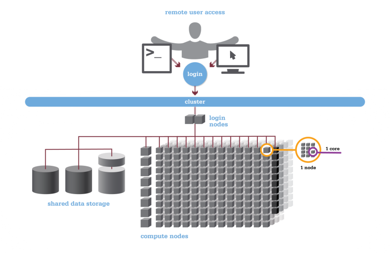
HPC Workflow
Using HPC is a little different from running programs on your desktop. When you login you’ll be connected to one of the system’s “login nodes”. These nodes serve as a staging area for you to marshal your data and submit jobs to the batch scheduler. Your job will then wait in a queue along with other researchers' jobs. Once the resources it requires become available, the batch scheduler will then run your job on a subset of our hundreds of “compute nodes”. You can see the overall structure in the diagram below.
HPC Citizenship
An important point about the diagram above is that OSC clusters are a collection of shared, finite resources. When you connect to the login nodes, you are sharing their resources (CPU cycles, memory, disk space, network bandwidth, etc.) with a few dozen other researchers. The same is true of the file servers when you access your home or project directories, and can even be true of the compute nodes.
For most day-to-day activities you should not have to worry about this, and we take precautions to limit the impact that others might have on your experience. That said, there are a few use cases that are worth watching out for:
-
The login nodes should only be used for light computation; any CPU- or memory-intensive operations should be done using the batch system. A good rule of thumb is that if you wouldn't want to run a task on your personal desktop because it would slow down other applications, you shouldn't run it on the login nodes. (See also: Interactive Jobs.)
-
I/O-intensive jobs should copy their files to fast, temporary storage, such as the local storage allocated to jobs or the Scratch parallel filesystem.
-
When running memory-intensive or potentially unstable jobs, we highly recommend requesting whole nodes. By doing so you prevent other users jobs from being impacted by your job.
-
If you request partial nodes, be sure to consider the amount of memory available per core. (See: HPC Hardware.) If you need more memory, request more cores. It is perfectly acceptable to leave cores idle in this situation; memory is just as valuable a resource as processors.
In general, we just encourage our users to remember that what you do may affect other researchers on the system. If you think something you want to do or try might interfere with the work of others, we highly recommend that you contact us at oschelp@osc.edu.
Getting Connected
There are two ways to connect to our systems. The traditional way will require you to install some software locally on your machine, including an SSH client, SFTP client, and optionally an X Windows server. The alternative is to use our zero-client web portal, OnDemand.
OnDemand Web Portal
OnDemand is our "one stop shop" for access to our High Performance Computing resources. With OnDemand, you can upload and download files, create, edit, submit, and monitor jobs, run GUI applications, and connect via SSH, all via a web broswer, with no client software to install and configure.
You can access OnDemand by pointing a web browser to ondemand.osc.edu. Documentation is available here. Any newer version of a common web brower should be sufficient to connect.
Using Traditional Clients
Required Software
In order to use our systems, you'll need two main pieces of software: an SFTP client and an SSH client.
SFTP ("SSH File Transfer Protocol") clients allow you transfer files between your workstation and our shared filesystem in a secure manner. We recommend the following applications:
- FileZilla: A high-performance open-source client for Windows, Linux, and OS X. A guide to using FileZilla is available here (external).
- CyberDuck: A high quality free client for Windows and OS X.
- sftp: The command-line utility sftp comes pre-installed on OS X and most Linux systems.
SSH ("Secure Shell") clients allow you to open a command-line-based "terminal session" with our clusters. We recommend the following options:
- PuTTY: A simple, open-source client for Windows.
- Secure Shell for Google Chrome: A free, HTML5-based SSH client for Google Chrome.
- ssh: The command-line utility ssh comes pre-installed on OS X and most Linux systems.
A third, optional piece of software you might want to install is an X Windows server, which will be necessary if you want to run graphical, windowed applications like MATLAB. We recommend the following X Windows servers:
- Xming: Xming offers a free version of their X Windows server for Microsoft Windows systems.
- X-Win32: StarNet's X-Win32 is a commercial X Windows server for Microsoft Windows systems. They offer a free, thirty-day trial.
- X11.app/XQuartz: X11.app, an Apple-supported version of the open-source XQuartz project, is freely available for OS X.
In addition, for Windows users, you can use OSC Connect, which is a native windows application developed by OSC to provide a launcher for secure file transfer, VNC, terminal, and web based services, as well as preconfigured management of secure tunnel connections. See this page for more information on OSC Connect.
Connecting via SSH
The primary way you'll interact with the OSC clusters is through the SSH terminal. See our supercomputing environments for the hostnames of our current clusters. You should not need to do anything special beyond entering the hostname.
Once you've established an SSH connection, you will be presented with some informational text about the cluster you've connected to followed by a UNIX command prompt. For a brief discussion of UNIX command prompts and what you can do with them, see the next section of this guide.
Transferring Files
To transfer files, use your preferred SFTP client to connect to:
sftp.osc.edu
You may see warning message including SSH key fingerprint. Verify that the fingerprint in the message matches one of the SSH key fingerprint listed here, then type yes.
Since process times are limited on the login nodes, trying to transfer large files directly to pitzer.osc.edu or other login nodes may terminate partway through. The sftp.osc.edu is specially configured to avoid this issue, and so we recommend it for all your file transfers.
Note: The sftp.osc.edu host is not connected to the scheduler, so you cannot submit jobs from this host. Use of this host for any purpose other than file transfer is not permitted.
Firewall Configuration
See our Firewall and Proxy Settings page for information on how to configure your firewall to allow connection to and from OSC.
Setting up X Windows (Optional)
With an X Windows server you will be able to run graphical applications on our clusters that display on your workstation. To do this, you will need to launch your X Windows server before connecting to our systems. Then, when setting up your SSH connection, you will need to be sure to enable "X11 Forwarding".
For users of the command-line ssh client, you can do this by adding the "-X" option. For example, the below will connect to the Pitzer cluster with X11 forwarding:
$ ssh -X username@pitzer.osc.edu
If you are connecting with PuTTY, the checkbox to enable X11 forwarding can be found in the connections pane under "Connections → SSH → X11".
For other SSH clients, consult their documentation to determine how to enable X11 forwarding.
NOTE: The X-Windows protocol is not a high-performance one. Depending on your system and Internet connection, X Windows applications may run very slowly, even to the point of being unusable. If you find this to be the case and graphical applications are a necessity for your work, please contact OSC Help to discuss alternatives.
Service:
Budgets and Accounts
The Ohio Supercomputer Center provides services to clients from a variety of types of organizations. The methods for gaining access to the systems are different between Ohio academic institutions and everyone else.
Ohio academic clients
Primarily, our users are Ohio-based and academic, and the vast majority of our resources will continue to be consumed by Ohio-based academic users. See the "Ohio Academic Fee Model FAQ" section on our service costs webpage.
Other clients
Other users (business, non-Ohio academic, nonprofit, hospital, etc.) interested in using Center resources may purchase services at a set rate available on our price list. Expert consulting support is also available.
Other computing centers
For users interested in gaining access to larger resources, please contact OSC Help. We can assist you in applying for resources at an NSF or XSEDE site.
Managing an OSC project
Once a project has been created, the PI can create accounts for users by adding them through the client portal. Existing users can also be added. More information can be found on the Project Menu documentation page.
I need additional resources for my existing project and/or I received an email my allocation is exhausted
If an academic PI wants a new project or to update the budget balance on an existing project(s), please see our creating projects and budget documentation.
I wish to use OSC to support teaching a class
We provide special classroom projects for this purpose and at no cost. You may use the client portal after creating an account. The request will need to include a syllabus or a similar document.
I don't think I fit in the above categories
Please contact us in order to discuss options for using OSC resources.
Project Applications
Application if you are employed by an Ohio Academic Institution
Use of computing resources and services at OSC is subject to the Ohio Supercomputer Center (OSC) Code of Ethics for Academic Users. Ohio Academic Clients are eligible for highly subsidized access to OSC resources, with fees only accruing after a credit provided is exhausted. Clients from an Ohio academic institution that expect to use more than the credit should consult with their institution on the proper guidance for requesting approval to be charged for usage. See the academic fee structure FAQ page for more information.
Eligible principal investigators (PIs) at Ohio academic institutions are able to request projects at OSC, but should also consult with their institution before incurring charges. In order to be an eligible PI at OSC, you must be eligible to hold PI status at your college, university, or research organization administered by an Ohio academic institution (i.e., be a full-time, permanent academic researcher or tenure-track faculty member at an Ohio college or university). Students, post-doctoral fellows, visiting scientists, and others who wish to use the facilities may be authorized users on projects headed by an eligible PI. Once a PI has received their project information, he/she can manage users for the project. Principal Investigators of OSC projects are responsible for updating their authorized user list, their outside funding sources, and their publications and presentations that cite OSC. All of these tasks can be accomplished by contacting using the client portal. Please review the documentation for more information. PIs are also responsible for monitoring their project's budget (balance) and for requesting a new budget (balance) before going negative, as projects with negative balances are restricted.
OSC's online project requests through our Client Portal is part of an electronic system that leads you through the process step by step. Before you begin to fill in the application form, especially if you are new to the process, look at the academic fee structure page. You can save a partially completed project request for later use.
If you need assistance, please contact OSC Help.
Application if you are NOT employed by an Ohio Academic Institution
Researchers from businesses, non-Ohio academic, nonprofits, hospitals or other organizations (which do not need to be based in Ohio) who wish to use the OSC's resources should complete the Other Client request form available here. All clients not affiliated with and approved by an Ohio academic institution must sign a service agreement, provide a $500 deposit, and pay for resource usage per a standard price list.
Letter of Commitment for Outside Funding Proposals
OSC will provide a letter of commitment users can include with their account proposals for outside funding, such as from the Department of Energy, National Institutes of Health, National Science Foundation (limited to standard text, per NSF policy), etc. This letter details OSC's commitment to supporting research efforts of its users and the facilities and platforms we provide our users. [Note: This letter does not waive the normal OSC budget process; it merely states that OSC is willing to support such research.] The information users must provide for the letter is:
- address to which the letter should be directed (e.g. NSF, Department, mailing address)
- name of funding agency's representative
- name of the proposal, as well as names and home institutions of the Co-PIs
- budget amount per year you would apply for if you were to receive funding
- number of years of proposed research
- solicitation number
Send e-mail with your request for the commitment letter to OSC Help or submit online. We will prepare a draft for your approval and then we will send you the final PDF for your proposal submission. Please allow at least two working days for this service.
Letter of Support for Outside Funding Proposals
Letters of support may be subject to strict and specific guidelines, and may not be accepted by your funding agency.
If you need a letter of support, please see above "Letter of Commitment for Outside Funding Proposals".
Applying at NSF Centers
Researchers requiring additional computing resources should consider applying for allocations at National Science Foundation Centers. For more information, please write to oschelp@osc.edu, and your inquiry will be directed to the appropriate staff member.:
We require you cite OSC in any publications or reports that result from projects supported by our services.
UNIX Basics
OSC HPC resources use an operating system called "Linux", which is a UNIX-based operating system, first released on 5 October 1991. Linux is by a wide margin the most popular operating system choice for supercomputing, with over 90% of the Top 500 list running some variant of it. In fact, many common devices run Linux variant operating systems, including game consoles, tablets, routers, and even Android-based smartphones.
While Linux supports desktop graphical user interface configurations (as does OSC) in most cases, file manipulation will be done via the command line. Since all jobs run in batch will be non-interactive, they by definition will not allow the use of GUIs. Thus, we strongly suggest new users become comfortable with basic command-line operations, so that they can learn to write scripts to submit to the scheduler that will behave as intended. We have provided some tutorials explaining basics from moving about the file system, to extracting archives, to modifying your environment, that are available for self-paced learning.
Linux Command Line Fundamentals
This tutorial teaches you about the linux command line and shows you some useful commands. It also shows you how to get help in linux by using the man and apropos commands.
Linux Tutorial
This tutorial guides you through the process of creating and submitting a batch script on one of our compute clusters. This is a linux tutorial which uses batch scripting as an example, not a tutorial on writing batch scripts. The primary goal is not to teach you about batch scripting, but for you to become familiar with certain linux commands that can be used either in a batch script or at the command line. There are other pages on the OSC web site that go into the details of submitting a job with a batch script.
Linux Shortcuts
This tutorial shows you some handy time-saving shortcuts in linux. Once you have a good understanding of how the command line works, you will want to learn how to work more efficiently.
Tar Tutorial
This tutorial shows you how to download tar (tape archive) files from the internet and how to deal with large directory trees of files.
Service:
Linux Command Line Fundamentals
Description
This tutorial teaches you about the linux command line and shows you some useful commands. It also shows you how to get help in linux by using the man and apropos commands.
For more training and practice using the command line, you can find many great tutorials. Here are a few:
https://www.learnenough.com/command-line-tutorial
https://cvw.cac.cornell.edu/Linux/
http://www.ee.surrey.ac.uk/Teaching/Unix/
https://www.udacity.com/course/linux-command-line-basics--ud595
More Advanced:
http://moo.nac.uci.edu/~hjm/How_Programs_Work_On_Linux.html
Prerequisites
None.
Introduction
Unix is an operating system that comes with several application programs. Other examples of operating systems are Microsoft Windows, Apple OS and Google's Android. An operating system is the program running on a computer (or a smartphone) that allows the user to interact with the machine -- to manage files and folders, perform queries and launch applications. In graphical operating systems, like Windows, you interact with the machine mainly with the mouse. You click on icons or make selections from the menus. The Unix that runs on OSC clusters gives you a command line interface. That is, the way you tell the operating system what you want to do is by typing a command at the prompt and hitting return. To create a new folder you type mkdir. To copy a file from one folder to another, you type cp. And to launch an application program, say the editor emacs, you type the name of the application. While this may seem old-fashioned, you will find that once you master some simple concepts and commands you are able to do what you need to do efficiently and that you have enough flexibility to customize the processes that you use on OSC clusters to suit your needs.
Common Tasks on OSC Clusters
What are some common tasks you will perform on OSC clusters? Probably the most common scenario is that you want to run some of the software we have installed on our clusters. You may have your own input files that will be processed by an application program. The application may generate output files which you need to organize. You will probably have to create a job script so that you can execute the application in batch mode. To perform these tasks, you need to develop a few different skills. Another possibility is that you are not just a user of the software installed on our clusters but a developer of your own software -- or maybe you are making some modifications to an application program so you need to be able to build the modified version and run it. In this scenario you need many of the same skills plus some others. This tutorial shows you the basics of working with the Unix command line. Other tutorials go into more depth to help you learn more advanced skills.
The Kernel and the Shell
You can think of Unix as consisting of two parts -- the kernel and the shell. The kernel is the guts of the Unix operating system -- the core software running on a machine that performs the infrastructure tasks like making sure multiple users can work at the same time. You don't need to know anything about the kernel for the purposes of this tutorial. The shell is the program that interprets the commands you enter at the command prompt. There are several different flavors of Unix shells -- Bourne, Korn, Cshell, TCshell and Bash. There are some differences in how you do things in the different shells, but they are not major and they shouldn't show up in this tutorial. However, in the interest of simplicity, this tutorial will assume you are using the Bash shell. This is the default shell for OSC users. Unless you do something to change that, you will be running the Bash shell when you log onto Owens or Pitzer.
The Command Prompt
The first thing you need to do is log onto one of the OSC clusters, Owens or Pitzer. If you do not know how to do this, you can find help at the OSC home page. If you are connecting from a Windows system, you need to download and setup the OSC Starter Kit which you can find here. If you are connecting from a Mac or Linux system, you will use ssh. To get more information about using ssh, go to the OSC home page, hold your cursor over the "Supercomputing" menu in the main blue menu bar and select "FAQ." This should help you get started. Once you are logged in look for the last thing displayed in the terminal window. It should be something like
-bash-3.2$
with a block cursor after it. This is the command prompt -- it's where you will see the commands you type in echoed to the screen. In this tutorial, we will abbreviate the command prompt with just the dollar sign - $. The first thing you will want to know is how to log off. You can log off of the cluster by typing "exit" then typing the <Enter> key at the command prompt:
$ exit <Enter>
For the rest of this tutorial, when commands are shown, the <Enter> will be omitted, but you must always enter <Enter> to tell the shell to execute the command you just typed.
First Simple Commands
So let's try typing a few commands at the prompt (remember to type the <Enter> key after the command):
$ date

$ cal

$ finger

$ who

$ whoami

$ finger -l
That last command is finger followed by a space then a minus sign then the lower case L. Is it obvious what these commands do? Shortly you will learn how to get information about what each command does and how you can make it behave in different ways. You should notice the difference between "finger" and "finger -l" -- these two commands seem to do similar things (they give information about the users who are logged in to the system) but they print the information in different formats. try the two commands again and examine the output. Note that you can use the scroll bar on your terminal window to look at text that has scrolled off the screen.
man
The "man" command is how you find out information about what a command does. Type the following command:
$ man
It's kind of a smart-alecky answer you get back, but at least you learn that "man" is short for "manual" and that the purpose is to print the manual page for a command. Before we start looking at manual pages, you need to know something about the way Unix displays them. It does not just print the manual page and return you to the command prompt -- it puts you into a mode where you are interactively viewing the manual page. At the bottom of the page you should see a colon (:) instead of the usual command prompt (-bash-3.2$). You can move around in the man page by typing things at the colon. To exit the man page, you need to type a "q" followed by <Enter>. So try that first. Type
$ man finger
then at the colon of the man page type
: q
You do not have to type <Enter> after the "q" (this is different from the shell prompt.) You should be back at the shell prompt now. Now let's go through the man page a bit. Once again, type
$ man finger
Now instead of just quitting, let's look at the contents of the man page. The entire man page is probably not displayed in your terminal. To scroll up or down, use the arrow keys or the <Page Up> and <Page Down> keys of the keyboard. The <Enter> and <Space> keys also scroll. Remember that "q" will quit out of the man page and get you back to the shell prompt.
The first thing you see is a section with the heading "NAME" which displays the name of the command and a short summary of what it does. Then there is a section called "SYNOPSIS" which shows the syntax of the command. In this case you should see
SYNOPSIS

     finger [-lmsp] [user ...] [user@host ...]
Remember how "finger" and "finger -l" gave different output? The [-lmsp] tells you that you can use one of those four letters as a command option -- i.e., a way of modifying the way the command works. In the "DESCRIPTION" section of the man page you will see a longer description of the command and an explanation of the options. Anything shown in the command synopsis which is contained within square brackets ([ ]) is optional. That's why it is ok to type "finger" with no options and no user. What about "user" -- what is that? To see what that means, quit out of the man page and type the following at the command prompt:
$ whoami
Let's say your username is osu0000. Then the result of the "whoami" command is osu0000. Now enter the following command (but replace osu0000 with your username):
$ finger osu0000
You should get information about yourself and no other users. You can also enter any of the usernames that are output when you enter the "finger" command by itself. The user names are in the leftmost column of output. Now try
$ finger -l osu0000

$ finger -lp osu0000

$ finger -s osu0000 osu0001
For the last command, use your username and the username of some other username that shows up in the output of the "finger" command with no arguments.
Note that a unix command consists of three parts:
- command
- option(s)
- argument(s)
You don't necessarily have to enter an argument (as you saw with the "finger" command) but sometimes a command makes no sense without an argument so you must enter one -- you saw this with the "man" command. Try typing
$ man man
and looking briefly at the output. One thing to notice is the synopsis -- there are a lot of possible options for the "man" command, but the last thing shown in the command synopsis is "name ..." -- notice that "name" is not contained in square brackets. This is because it is not optional -- you must enter at least one name. What happens if you enter two names?
$ man man finger
The first thing that happens is you get the man page for the "man" command. What happens when you quit out of the man page? You should now get the man page for the "finger" command. If you quit out of this one you will be back at the shell prompt.
Combining Commands
You can "pipe" the output of one command to another. First, let's learn about the "more" command:
$ man more
Read the "DESCRIPTION" section -- it says that more is used to page through text that doesn't fit on one screen. It also recommends that the "less" command is more powerful. Ok, so let's learn about the "less" command:
$ man less
You see from the description that "less" also allows you to examine text one screenful at a time. Does this sound familiar? The "man" command actually uses the "less" command to display its output. But you can use the "less" command yourself. If you have a long text file named "foo.txt" you could type
$ less foo.txt
and you would be able to examine the contents of the file one screen at a time. But you can also use "less" to help you look at the output of a command that prints more than one screenful of output. Try this:
$ finger | less
That's "finger" followed by a space followed by the vertical bar (shifted backslash on most keyboards) followed by a space followed by "less" followed by <Enter>. You should now be looking at the output of the "finger" command in an interactive fashion, just as you were looking at man pages. Remember, to scroll use the arrow keys, the <Page Up> and <Page Down> keys, the <Enter> key or the space bar; and to quit, type "q".
Now try the following (but remember to replace "osu0000" with your actual username):
$ finger | grep osu0000
The "grep" command is Unix's command for searching. Here you are telling Unix to search the output of the "finger" command for the text "osu0000" (or whatever your username is.)
If you try to pipe the output of one command to a second command and the second is a command which works with no arguments, you won't get what you expect. Try
$ whoami | finger
You see that it does not give the same output as
$ finger osu0000
(assuming "whoami" returns osu0000.)
In this case what you can do is the following:
$ finger `whoami`
That's "finger" space backquote "whoami" backquote. The backquote key is to the left of the number 1 key on a standard keyboard.
apropos
Enter the following command:
$ man apropos
As you can see, the apropos searches descriptions of commands and finds commands whose descriptions match the keyword you entered as the argument. That means it outputs a list of commands that have something to do with the keyword you entered. Try this
$ apropos
Ok, you need to enter an argument for the "apropos" command.
So try
$ apropos calendar
Now you see that among the results are two commands -- "cal" and "difftime" that have something to do with the keyword "calendar."
Linux Tutorial
Description
This tutorial guides you through the process of creating and submitting a batch script on one of our compute clusters. This is a linux tutorial which uses batch scripting as an example, not a tutorial on writing batch scripts. The primary goal is not to teach you about batch scripting, but for you to become familiar with certain linux commands. There are other pages on the OSC web site that go into the details of submitting a job with a batch script.
Prerequisites
- Familiarity with a text editor (emacs, nano, vim)
- Basic understanding of the unix command line
- Linux Command Line Fundamentals tutorial
Goals
- Create subdirectories to organize information
- Create a batch script with a text editor
- Submit a job
- Check on the progress of the job
- Change the permissions of the output files
- Get familiar with some common unix commands
Step 1 - Organize your directories
When you first log in to our clusters, you are in your home directory. For the purposes of this illustration, we will pretend you are user osu0001 and your project code is PRJ0001, but when you try out commands you must use your own username and project code.
$ pwd
/users/PRJ0001/osu0001
Note: you will see your user name and a different number after the /users.
It's a good idea to organize your work into separate directories. If you have used Windows or the Mac operating system, you may think of these as folders. Each folder may contain files and subfolders. The subfolders may contain other files and subfolders of their own. In linux we use the term "directory" instead of "folder." Use directories to organize your work.
Type the following four lines and take note of the output after each one:
$ touch foo1
$ touch foo2
$ ls
$ ls -l
$ ls -lt
$ ls -ltr
The "
touch" command just creates an empty file with the name you give it.You probably already know that the ls command shows the contents of the current working directory; that is, the directory you see when you type pwd. But what is the point of the "
-l", "-lt" or "-ltr"? You noticed the difference in the output between just the "ls" command and the "ls -l" command.Most unix commands have options you can specify that change the way the command works. The options can be specified by the "
-" (minus sign) followed by a single letter. "ls -ltr" is actually specifying three options to the ls command.l: I want to see the output in long format -- one file per line with some interesting information about each filet: sort the display of files by when they were last modified, most-recently modified firstr: reverse the order of display (combined with -t this displays the most-recently modified file last -- it should be BatchTutorial in this case.)I like using "
ls -ltr" because I find it convenient to see the most recently modified file at the end of the list.Now try this:
$ mkdir BatchTutorial
$ ls -ltr
The "
mkdir" command makes a new directory with the name you give it. This is a subfolder of the current working directory. The current working directory is where your current focus is in the hierarchy of directories. The 'pwd' command shows you are in your home directory:$ pwd /users/PRJ0001/osu0001
Now try this:
$ cd BatchTutorial
$ pwd
What is the output of '
pwd' now? "cd" is short for "change directory" -- think of it as moving you into a different place in the hierarchy of directories. Now do$ cd .. $ pwd
Where are you now?
Step 2 -- Get familiar with some more unix commands
Try the following:
$ echo where am I?
$ echo I am in `pwd`
$ echo my home directory is $HOME
$ echo HOME
$ echo this directory contains `ls -l`
These examples show what the echo command does and how to do some interesting things with it. The `pwd` means the result of issuing the command pwd. HOME is an example of an environment variable. These are strings that stand for other strings. HOME is defined when you log in to a unix system. $HOME means the string the variable HOME stands for. Notice that the result of "echo HOME" does not do the substitution. Also notice that the last example shows things don't always get formatted the way you would like.
Some more commands to try:
$ cal
$ cal > foo3
$ cat foo3
$ whoami
$ date
Using the ">" after a command puts the output of the command into a file with the name you specify. The "cat" command prints the contents of a file to the screen.
Two very important UNIX commands are the cp and mv commands. Assume you have a file called foo3 in your current directory created by the "cal > foo3" command. Suppose you want to make a copy of foo3 called foo4. You would do this with the following command:
$ cp foo3 foo4
$ ls -ltr
Now suppose you want to rename the file 'foo4' to 'foo5'. You do this with:
$ mv foo4 foo5
$ ls -ltr
'mv' is short for 'move' and it is used for renaming files. It can also be used to move a file to a different directory.
$ mkdir CalDir
$ mv foo5 CalDir
$ ls
$ ls CalDir
Notice that if you give a directory with the "ls" command is shows you what is in that directory rather than the current working directory.
Now try the following:
$ ls CalDir
$ cd CalDir
$ ls
$ cd ..
$ cp foo3 CalDir
$ ls CalDir
Notice that you can use the "cp" command to copy a file to a different directory -- the copy will have the same name as the original file. What if you forget to do the mkdir first?
$ cp foo3 FooDir
Now what happens when you do the following:
$ ls FooDir
$ cd FooDir
$ cat CalDir
$ cat FooDir
$ ls -ltr
CalDir is a directory, but FooDir is a regular file. You can tell this by the "d" that shows up in the string of letters when you do the "ls -ltr". That's what happens when you try to cp or mv a file to a directory that doesn't exist -- a file gets created with the target name. You can imagine a scenario in which you run a program and want to copy the resulting files to a directory called Output but you forget to create the directory first -- this is a fairly common mistake.
Step 3 -- Environment Variables
Before we move on to creating a batch script, you need to know more about environment variables. An environment variable is a word that stands for some other text. We have already seen an example of this with the variable HOME. Try this:
$ MY_ENV_VAR="something I would rather not type over and over"
$ echo MY_ENV_VAR
$ echo $MY_ENV_VAR
$ echo "MY_ENV_VAR stands for $MY_ENV_VAR"
You define an environment variable by assigning some text to it with the equals sign. That's what the first line above does. When you use '$' followed by the name of your environment variable in a command line, UNIX makes the substitution. If you forget the '$' the substitution will not be made.
There are some environment variables that come pre-defined when you log in. Try using 'echo' to see the values of the following variables: HOME, HOSTNAME, SHELL, TERM, PATH.
Now you are ready to use some of this unix knowledge to create and run a script.
Step 4 -- Create and run a script
Before we create a batch script and submit it to a compute node, we will do something a bit simpler. We will create a regular script file that will be run on the login node. A script is just a file that consists of unix commands that will run when you execute the script file. It is a way of gathering together a bunch of commands that you want to execute all at once. You can do some very powerful things with scripting to automate tasks that are tedious to do by hand, but we are just going to create a script that contains a few commands we could easily type in. This is to help you understand what is happening when you submit a batch script to run on a compute node.
Use a text editor to create a file named "tutorial.sh" which contains the following text (note that with emacs or nano you can use the mouse to select text and then paste it into the editor with the middle mouse button):
$ nano tutorial.sh
echo ----
echo Job started at `date`
echo ----
echo This job is working on node `hostname`

SH_WORKDIR=`pwd`
echo working directory is $SH_WORKDIR
echo ----
echo The contents of $SH_WORKDIR
ls -ltr
echo
echo ----
echo
echo creating a file in SH_WORKDIR
whoami > whoami-sh-workdir

SH_TMPDIR=${SH_WORKDIR}/sh-temp
mkdir $SH_TMPDIR
cd $SH_TMPDIR
echo ----
echo TMPDIR IS `pwd`
echo ----
echo wait for 12 seconds
sleep 12
echo ----
echo creating a file in SH_TMPDIR
whoami > whoami-sh-tmpdir

# copy the file back to the output subdirectory
cp ${SH_TMPDIR}/whoami-sh-tmpdir ${SH_WORKDIR}/output

cd $SH_WORKDIR

echo ----
echo Job ended at `date`
To run it:
$ chmod u+x tutorial.sh
$ ./tutorial.sh
Look at the output created on the screen and the changes in your directory to see what the script did.
Step 5 -- Create and run a batch job
Use your favorite text editor to create a file called tutorial.pbs in the BatchTutorial directory which has the following contents (remember, you can use the mouse to cut and paste text):
#PBS -l walltime=00:02:00
#PBS -l nodes=1:ppn=1
#PBS -N foobar
#PBS -j oe
#PBS -r n

echo ----
echo Job started at `date`
echo ----
echo This job is working on compute node `cat $PBS_NODEFILE`

cd $PBS_O_WORKDIR
echo show what PBS_O_WORKDIR is
echo PBS_O_WORKDIR IS `pwd`
echo ----
echo The contents of PBS_O_WORKDIR:
ls -ltr
echo
echo ----
echo
echo creating a file in PBS_O_WORKDIR
whoami > whoami-pbs-o-workdir

cd $TMPDIR
echo ----
echo TMPDIR IS `pwd`
echo ----
echo wait for 42 seconds
sleep 42
echo ----
echo creating a file in TMPDIR
whoami > whoami-tmpdir

# copy the file back to the output subdirectory
pbsdcp -g $TMPDIR/whoami-tmpdir $PBS_O_WORKDIR/output

echo ----
echo Job ended at `date`
To submit the batch script, type
$ qsub tutorial.pbs
Use
qstat -u [username] to check on the progress of your job. If you see something like this
$ qstat -u osu0001

                                                                             Req'd  Req'd   Elap
Job ID             Username    Queue    Jobname          SessID NDS   TSK    Memory Time  S Time
------------------ ----------- -------- ---------------- ------ ----- ------ ------ ----- - -----
458842.oak-batch   osu0001     serial   foobar              --      1      1    --  00:02 Q   --
this means the job is in the queue -- it hasn't started yet. That is what the "Q" under the S column means.
If you see something like this:
                                                                             Req'd  Req'd   Elap
Job ID             Username    Queue    Jobname          SessID NDS   TSK    Memory Time  S Time
------------------ ----------- -------- ---------------- ------ ----- ------ ------ ----- - -----
458842.oak-batch   osu0001     serial   foobar            26276     1      1    --  00:02 R   --
this means the job is running and has job id 458842.
When the output of the
qstat command is empty, the job is done.After it is done, there should be a file called "foobar.o458842" in the directory.
Note that your file will end with a different number -- namely the job id number assigned to your job.
Check this with
$ ls -ltr
$ cat foobar.oNNNNNN
Where (NNNNNN is your job id).
The name of this file is determined by two things:
- The name you give the job in the script file with the header line #PBS -N foobar
- The job id number assigned to the job.
The name of the script file (tutorial.pbs) has nothing to do with the name of the output file.
Examine the contents of the output file foobar.oNNNNNN carefully. You should be able to see the results of some of the commands you put in tutorial.pbs. It also shows you the values of the variables PBS_NODEFILE, PBS_O_WORKDIR and TMPDIR. These variables exist only while your job is running. Try
$ echo $PBS_O_WORKDIR
and you will see it is no longer defined. $PBS_NODEFILE is a file which contains a list of all the nodes your job is running on. Because this script has the line
#PBS -l nodes=1:ppn=1
the contents of $PBS_NODEFILE is the name of a single compute node.
Notice that $TMPDIR is /tmp/pbstmp.NNNNNN (again, NNNNNN is the id number for this job.) Try
$ ls /tmp/pbstmp.NNNNNN
Why doesn't this directory exist? Because it is a directory on the compute node, not on the login node. Each machine in the cluster has its own /tmp directory and they do not contain the same files and subdirectories. The /users directories are shared by all the nodes (login or compute) but each node has its own /tmp directory (as well as other unshared directories.)
Tar Tutorial
Prerequisites
Step 1 -- Create a directory to work with and download a "tarball"
Start off with the following:
$ mkdir TarTutorial
$ cd TarTutorial
$ wget http://www.mmm.ucar.edu/wrf/src/WRFDAV3.1.tar.gz
$ ls -ltr
The third command will take a while because it is downloading a file from the internet. The file is call a "tarball" or a "gzipped tarball". TAR is an old unix short name for "tape archive" but a tar file is a file that contains a bunch of other files. If you have to move a bunch of files from one place to another, a good way to do it is to pack them into a tar file, move the tar file where you want it then unpack the files at the destination. A tar file usually has the extension ".tar". What about the ".gz"? This means the tar file has been further compressed with the program gzip -- this makes it a lot smaller.
Step 2 -- Unpack the "tarball" and check out the contents
After step 1 your working directory should be ~/TarTutorial and there should be a file called WRFDAV3.1.tar.gz in it.
Now do this:
$ gunzip WRFDAV3.1.tar.gz
$ ls -ltr
You should now have a file called WRFDAV3.1.tar which should be quite a bit larger in size than WRFDAV3.1.tar.gz -- this is because it has been uncompressed by the "gunzip" command which is the opposite of the "gzip" command.
Now do this:
$ tar -xvf WRFDAV3.1.tar
$ ls -ltr
You should see a lot of filenames go by on the screen and when the first command is done and you issue the ls command you should see two things -- WRFDAV3.1.tar is still there but there is also a directory called WRFDA. You can look at the contents of this directory and navigate around in the directory tree to see what is in there. The options on the "tar" command have the following meanings (you can do a "man tar" to get all the options):
x: extract the contents of the tar file
v: be verbose, i.e. show what is happening on the screen
f: the name of the file which follows the "f" option is the tar file to expand.
Another thing you can do is see how much space is being taken up by the files. Make sure TarTutorial is your working directory then issue the following command:
$ du .
Remember that "." (dot) means the current working directory. The "du" command means "disk usage" -- it shows you how much space is being used by every file and directory in the directory tree. It ends up with the highest level files and directories. You might prefer to do
$ du -h .
$ ls -ltrh
Adding the "-h" option to these commands puts the file sizes in human-readable format -- you should get a size of 66M for the tar file -- that's 66 megabytes -- and "du" should print a size of 77M next to ./WRFDA.
Step 3 -- create your own "tarball"
Now, make your own tar file from the WRFDA directory tree:
$ tar -cf mywrf.tar WRFDA
$ ls -ltrh
You have created a tar from all the files in the WRFDA directory. The options given to the "tar" command have the following meanings:
c: create a tar file
f: give it the name which follows the "f" option
The files WRFDAV3.1.tar and mywrf.tar are identical. Now compress the tar file you made:
$ gzip mywrf.tar
$ ls -ltrh
You should see a file called mywrf.tar.gz which is smaller than WRFDAV3.1.tar.
Step 4 -- Clean up!
You don't want to leave all these files lying around. So delete them
$ rm WRFDAV3.1.tar
$ rm mywrf.tar
$ rm WRFDA
Oops! You can't remove the directory. You need to use the "rmdir" command:
$ rmdir WRFDA
Oh no! That doesn't work on a directory that's not empty. So are you stuck with all those files? Maybe you can do this:
$ cd WRFDA
$ rm *
$ cd ..
$ rmdir WRFDA
That won't work either because there are some subdirectories in WRFDA and "rm *" won't remove them. Do you have to work your way to the all the leaves at the bottom of the directory tree and remove files then come back up and remove directories? No, there is a simpler way:
$ rm -Rf WRFDA
This will get rid of the entire directory tree. The options have the following meanings:
R: recursively remove all files and directories
f: force; i.e., just remove everything without asking for confirmation
I encourage you to do
$ man rm
and check out all the options. Or some of them -- there are quite a few.
Unix Shortcuts
Description
This tutorial shows you some handy time-saving shortcuts in linux. Once you have a good understanding of how the command line works, you will want to learn how to work more efficiently.
Prerequisites
Linux command line fundamentals.
Goals
- Save you time when working on a linux system
- Increase your appreciation of the power of linux
Step 1 -- The Arrow Keys
Note: even if you know how to use the up arrow in linux, you need to enter the commands in this section because they are used in the following sections. So to begin this tutorial, go to your home directory and create a new directory called ShortCuts:
$ cd
$ mkdir Shortcuts
$ cd Shortcuts
(If a directory or file named "Shortcuts" already exists, name it something else.)
Imagine typing in a long linux command and making a typo. This is one of the frustrating things about a command line interface -- you have to retype the command, correcting the typo this time. Or what if you have to type several similar commands -- wouldn't it be nice to have a way to recall a previous command, make a few changes, and enter the new command? This is what the up arrow is for.
Try the following:
$ cd ..
$ cd ShortCuts (type a capital C)
Linux should tell you there is no directory with that name.
Now type the up arrow key -- the previous command you entered shows up on the command line, and you can use the left arrow to move the cursor just after the capital C, hit Backspace, and type a lower case c. Note you can also position the cursor before the capital C and hit Delete to get rid of it.
Once you have changed the capital C to a lower case c you can hit Return to enter the command -- you do not have to move the cursor to the end of the line.
Now hit the up arrow key a few times, then hit the down arrow key and notice what happens. Play around with this until you get a good feel for what is happening.
Linux maintains a history of commands you have entered. Using the up and down arrow keys, you can recall previously-entered commands to the command line, edit them and re-issue them.
Note that in addition to the left and right arrow keys you can use the Home and End keys to move to the beginning or end of the command line. Also, if you hold down the Ctrl key when you type an arrow key, the cursor will move by an entire word instead of a single character -- this is useful is many situations and works in many editors.
Let's use this to create a directory hierarchy and a few files. Start in the Shortcuts directory and enter the following commands, using the arrow keys to simplify your job:
$ mkdir directory1
$ mkdir directory1/directory2
$ mkdir directory1/directory2/directory3
$ cd directory1/directory2/diectoryr3  (remember the Home key and the Ctrl key with left and right arrows)
$ hostname > file1
$ whoami > file2
$ mkdir directory4
$ cal > directory4/file3
Step 2 -- Using the TAB key
Linux has short, cryptic command names to save you typing -- but it is still a command line interface, and that means you interact with the operating system by typing in commands. File names can be long, directory hierarchies can be deep, and this can mean you have to type a lot to specify the file you want or change to current working directory. Not only that, but you have to remember the names of files and directories you type in. The TAB key gives you a way to enter with commands with less typing and less memorization.
Go back to the Shortcuts directory:
$ cd
$ cd Shortcuts
Now enter the following:
$ hostname > file1
$ cal > file2
$ whoami > different-file
$ date > other-file
$ cal > folio5
Now type the following, without hitting the Return key:
$ cat oth <Tab>
What happened? Linux completed the name "other-file" for you! The Tab key is your way of telling Linux to finish the current word you are typing, if possible. Because there is only one file in the directory whose name begins with "oth", when you hit the Tab key Linux is able to complete the name.
Hit Return (if you haven't already) to enter the cat command. Now try
$ cat d <Tab>
As you would expect, Linux completes the name "different-file"
What if you enter
$ cat fi <Tab>
Notice Linux completes as much of the name as possible. You can now enter a "1" or a "2" to finish it off.
But what if you forget what the options are? What if you can't remember if you created "file1" and "file2" or if you created "fileA" and fileB"?
With the comman line showing this:
$ cat file
hit the Tab key twice. Aha! Linux shows you the possible choices for completing the word.
Try
$ cat f <Tab>
The Tab will not add anything -- the command line will still read
$ cat f
Now type the letter o followed by a Tab -- once you add the o there is only one possible completion -- "folio".
Now enter the following:
$ cat directory1/directory2/directory3/directory4/file3
That's kind of a painful to type.
Now type the following without entering Return:
$ ls dir <Tab>
Nice! As you would expect, Linux completes the name of the directory for you. This is because there is only one file in the Shortcuts directory whose name begins with "dir"
Hit Return and Linux will tell you that directory1 contains directory2.
Now type this:
$ ls dir <Tab>
and before you hit return type another d followed by another Tab. Your command line should now look like this:
$ ls directory1/directory2/
If you hit Return, Linux will tell you that directory2 contains directory3.
Now try this:
$ ls dir <Tab>
then type another d followed by <Tab> then another d followed by tab. Don't hit Return yet. Your command line should look like this:
$ ls directory1/directory2/directory3/
Don't hit Return yet. Now type the letter f followed by a Tab. What do you think should happen?
Step 3 -- The Exclamation Point
Hitting the up arrow key is a nice way to recall previously-used commands, but it can get tedious if you are trying to recall a command you entered a while ago -- hitting the same key 30 times is a good way to make yourself feel like an automaton. Fortunately, linux offers a couple of other ways to recall previous commands that can be useful.
Go back to the Shortcuts directory
$ cd ~/Shortcuts
and enter the following:
$ hostname
$ cal
$ date
$ whoami
Now enter this:
$ !c
and hit return.
What happened? Now try
$ !h
and hit return.
The exclamation point ("bang" to Americans, "shriek" to some Englishmen I've worked with) is a way of telling linux you want to recall the last command which matches the text you type after it. So "!c" means recall the last command that starts with the letter c, the "cal" command in this case. You can enter more than one character after the exclamation point in order to distinguish between commands. For example if you enter
$ cd ~/Shortcuts
$ cat file1
$ cal
$ !c
the last command will redo the "cal" command. But if you enter
$ cat file1
$ cal
$ !cat
the last command re-executes the "cat" command.
Step 4 -- Ctrl-r
One problem with using the exclamation point to recall a previous command is that you can feel blind -- you don't get any confirmation about exactly which command you are recalling until it has executed. Sometimes you just aren't sure what you need to type after the exclamation point to get the command you want.
Typing Ctrl-r (that's holding down the Ctrl key and typing a lower case r) is another way to repeat previous commands without having to type the whole command, and it's much more flexible than the bang. The "r" is for "reverse search" and what happens is this. After you type Ctrl-r, start typing the beginning of a previously entered command -- linux will search, in reverse order, for commands that match what you type. To see it in action, type in the following commands (but don't hit <Enter> after the last one):
$ cd ~/Shortcuts
$ cat file1
$ cat folio5
$ cal
$ Ctrl-r cat
You should see the following on your command line:
(reverse-i-search)`cat': cat folio5
Try playing with this now. Type in " fi" (that's a space, an "f" and an "i") -- did the command shown at the prompt change? Now hit backspace four times.
Now enter a right or left arrow key and you will find yourself editing the matching command. This is one you have to play around with a bit before you understand exactly what it is doing. So go ahead and play with it.
Step 5 -- history
Now type
$ history
and hit return.
Cool, huh? You get to see all the commands you have entered (probably a maximum of 1000.) You can also do something like
$ history | grep cal
to get all the commands with the word "cal" in them. You can use the mouse to cut and paste a previous command, or you can recall it by number with the exclamation point:
$ !874
re-executes the command number 874 in your history.
For more information about what you can do to recall previous commands, check out http://www.thegeekstuff.com/2011/08/bash-history-expansion/
Step 6 -- Ctrl-t
I am just including this because to me it is a fun piece of linux trivia. I don't find it particularly useful. Type
$ cat file1
and hit <Return>. Now hit the up arrow key to recall this command and hist the left arrow key twice so the cursor is on the "e" of "file1". Now hit Ctrl-t (again, hold down the control key and type a lower case t.) What just happened? Try hitting Ctrl-t a couple more times. That's right -- it transposes two characters in the command line -- the one the cursor is on and the one to its left. Also, it moves the cursor to the right. Frankly, it takes me more time to think about what is going to happen if I type Ctrl-t than it takes me to delete some characters and retype them in the correct order. But somewhere out there is a linux black belt who gets extra productivity out of this shortcut.
Step 7 -- The alias command
Another nice feature of linux is the alias command. If there is a command you enter a lot you can define a short name for it. For example, we have been typing "cat folio5" a lot in this tutorial. You must be getting sick of typing "cat folio5". So enter the following:
$ alias cf5='cat folio5'
Now type
$ cf5
and hit return. Nice -- you now have a personal shortcut for "cat folio5". I use this for the ssh commands:
$ alias gogl='ssh -Y jeisenl@pitzer.osc.edu'
I put this in the .bash_aliases file on my laptop so that it is always available to me.
Classroom Project Resource Guide
This document includes information on utilizing OSC resources in your classroom effectively.
Request a Classroom Project
Classroom projects will not be billed under the Ohio academic fee structure; all fees will be fully discounted at the time of billing.
Please submit a new project request for a classroom project. You will request a $500 budget. If an additional budget is needed or you want to re-use your project code, you can apply through MyOSC or contact us at OSCHelp. We require a class syllabus; this will be uploaded on the last screen before you submit the request.
During setup, OSC staff test accounts may be added to the project for troubleshooting purposes.
Access
We suggest that students consider connecting to our OnDemand portal to access the HPC resources. All production supercomputing resources can be accessed via that website without having to worry about client configuration. We have a guide for new students to help them figure out the basics of using OSC.
If your class has set up a custom R or Jupyter environment at OSC, please ask the students to connect to
class.osc.eduResources
We currently have two production clusters, Pitzer and Owens, with Nvidia GPUs available that may be used for classroom purposes. All systems have "debug" queues that, during typical business hours, allow small jobs of less than one hour to start much quicker than they might otherwise.
If you need to reserve access to particular resources, please contact OSC Help, preferably with at least two weeks lead time, so that we can put in the required reservations to ensure resources are available during lab or class times.
Software
We have a list of supported software, including sample batch scripts, in our documentation. If you have specific needs that we can help with, let OSC Help know.
If you are using Rstudio, please see this webpage.
If you are using Jupyter, please see the page Using Jupyter for Classroom.
Account Maintenance
Our classroom project information guide will instruct you on how to get students added to your project using our client portal. For more information, see the documentation. You must also add your username as an authorized user.
Homework Submissions
We can provide you with project space to have students submit assignments through our systems. Please ask about this service and see our how-to. We typically grant 1-5 TB for classroom projects.
Support
Help can be found by contacting OSC Help weekdays, 9 a.m. to 5 p.m. (614-292-1800).
Fill out a request online.
We update our web pages to show relevant events at the center (including training) and system notices on our main page (osc.edu). We also provide important information in the “message of the day” (visible when you log in). You also can receive notices by following @HPCNotices on X.
Helpful Links
FAQ: http://www.osc.edu/supercomputing/faq
Main supercomputing pages: http://www.osc.edu/supercomputing/
Documentation Attachment:
Classroom Guide for Students
Join a Classroom Project
Your classroom instructor will provide you with a project and access code that will allow you to join the classroom project. Visit our user management page for more information.
Ohio State users only: osu.edu and buckeyemail.osu.edu are treated as two separate emails in our system. Please provide your professor the appropriate email address.
All emails will be sent from "no-reply@osc.edu" - all folders should be checked, including spam/junk. If they did not receive this email, please contact OSC Help.
Review our classroom project info guide for detailed informatoin.
Account Management
You can manage your OSC account via MyOSC, our client porta. This includes:
Access
If your class uses a custom R or Jupyter environment at OSC, please connect to class.osc.edu
If you do not see your class there, we suggest connecting to ondemand.osc.edu.
You can log into class.osc.edu or ondemand.osc.edu either using your OSC HPC Credentials or Third-Party Credentials. See this OnDemand page for more information.
File Transfer
There are a few different ways of transferring files between OSC storage and your local computer. We suggest using OnDemand File App if you are new to Linux and looking to transfer smaller-sized files - measured in MB to several hundred MB. For larger files, please use an SFTP client to connect to sftp.osc.edu or Globus.
More Information for New Users
We have a guide for new users to help them figure out the basics of using OSC; included are basics on getting connected, HPC system structure, file transfers, and batch systems.
FAQ: http://www.osc.edu/supercomputing/faq
Main Supercomputing pages: http://www.osc.edu/supercomputing/
Support
Help can be found by contacting OSC Help weekdays, 9AM to 5PM (614-292-1800).
Fill out a request online.
Documentation Attachment:
Using Jupyter for Classroom
OSC provide an isolated and custom Jupyter environment for each classroom project that requires Jupyter Notebook or JupyterLab.
The instructor must apply for a classroom project that is unique for the course. More details on the classroom project can be found in our classroom project guide. Once we get the information, we will provide you a project ID and a course ID (which is commonly the course ID provided by instructor + school code, e.g. MATH_2530_OU). The instructor can set up a Jupyter environment for the course using the information (see below). The Jupyter environment will be tied to the project ID.
Set up a Jupyter environment
The instructor can set up a Jupyter environment for the course once the project space is initialized:
- Login to Owens or Pitzer as PI account of the classroom project.
- Run setup script with the
project IDandcourse ID:
~support/classroom/tools/setup_jupyter_classroom /fs/ess/project_ID course_ID
If the Jupyter environment is created successfully, please inform us so we can update you when your class is ready at class.osc.edu.
Upgrade a Jupyter environment
You may need to upgrade Jupyter kernels to the latest stable version for a security vulnerability or trying out new features. Please run upgrade script with the project ID and course ID:
~support/classroom/tools/upgrade_jupyter_classroom /fs/ess/project_ID course_ID
Manage the Jupyter environment
Install packages
When your class is ready, launch your class session at class.osc.edu. Then, open a notebook and use the following command to install packages:
pip install --no-cache-dir --ignore-installed [package-name]
Please note that using the --no-cache-dir and --ignore-installed flags can skip using the caches in the home directory, which may cause conflicts when installing classroom packages if you have previously used pip to install packages in multiple Python environments.
Install extensions
Jupyter Notebook
To enable or install nbextension, please use --sys-prefix to install into the classroom Jupyter environment, e.g.
!jupyter contrib nbextension install --sys-prefix
Please do not use --user, which install to your home directory and could mess up the Jupyter environment.
JupyterLab
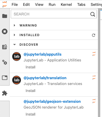
To install labextension, simply click Extension Manager icon at the side bar
Enable local package access (optional)
By default this Jupyter environment is an isolated Python environment. Anyone launches python from this environment can only access packages installed inside unless PYTHONPATH is used. The instructor can change it by setting include-system-site-packages = true in /fs/ess/project_ID/course_ID/jupyter/pyvenv.cfg. This will allows students to access packages in home directory ~/.local/lib/pythonX.X/site-packages ,and install packages via pip install –user
Workspace
When a class session starts, we create a classroom workspace under the instructor's and students' home space: $HOME/osc_classes/course_ID, and launch Jupyter at the workspace. The root / will appear in the landing page (Files) but everything can be found in $HOME/osc_classes/course_ID on OSC system.
Shared Access
Share class material
The instructor can upload class material to /fs/ess/project_ID/course_ID/materials . When a student launch a Jupyter session, the diretory will be copied to the student's worksapce $HOME/osc_classes/course_ID . The student will see the directory materials on the landing page. PI can add files to the material source directory. New files will be copied to the destination every time when a new Jupyter session starts. But If PI modifies existing files, the changes won't be copied as the files were copied before. Therefore we recommend renaming the file after the update so that it will be copied
If a large amount of data is added to /materials dir, then students may experience job failures. This is because there is not enough time for the data to be copied to their home dir.
Use data dir for large files
For large files, create a data dir to the classroom and place the large files there.
mkdir /fs/ess/project_ID/course_ID/data
Now the large data will not be copied to each user's home dir when they start a classroom job session. Make sure to reference this data properly in notebooks that will be copied to students home dirs from the /materials dir.
Access student workspace
The instructor and TAs can access a student's workspace with limited permissions. First, the instructor sends us a request with the information including the instructor's and TAs' OSC accounts. After a student launches a class session, you can access known files and directories in the student's workspace. For example, you cannot explore the student's workspace
ls /users/PZS1234/student1/osc_classes/course_ID
ls: cannot open directory /users/PZS1234/student1/osc_classes/course_ID: Permission denied
but you can access a known file or directory in the workspace
ls /users/PZS1234/student1/osc_classes/course_ID/homework
Using Rstudio for classroom
OSC provides an isolated and custom R environment for each classroom project that requires Rstudio. The interface can be accessed at class.osc.edu. Before using this interface, please apply for a classroom project account that is unique for the course. More details on the classroom project can be found here. The custom R environment for the course will be tied to this project ID. Please inform us if you have additional requirements for the class. Once we get the information, we will provide you a course_ID (which is commonly the course ID provided by instructor + school code, e.g. MATH2530_OU)and add your course to the server with the class module created using the course_ID. After login to the class.osc.edu server, you will see several Apps listed. Pick Rstudio server and that will take you to the Rstudio Job submission page. Please pick your course from the drop-down menu under the Class materials and the number of hours needed.
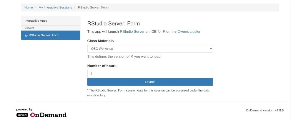
Clicking on the Launch will submit the Rstudio job to the scheduler and you will see Connect to Rstudio server option when the resource is ready for the job. Each Rstudio launch will run on 1 core on Owens machine with 4GB of memory.

Rstudio will open up in a new tab with a custom and isolated environment that is set through a container-based solution. This will create a folder under $HOME/osc_classes/course_ID for each user. Please note that inside the Rstudio, you won't be able to access any files other than class materials. However, you can access the class directory outside of Rstudio to upload or download files.
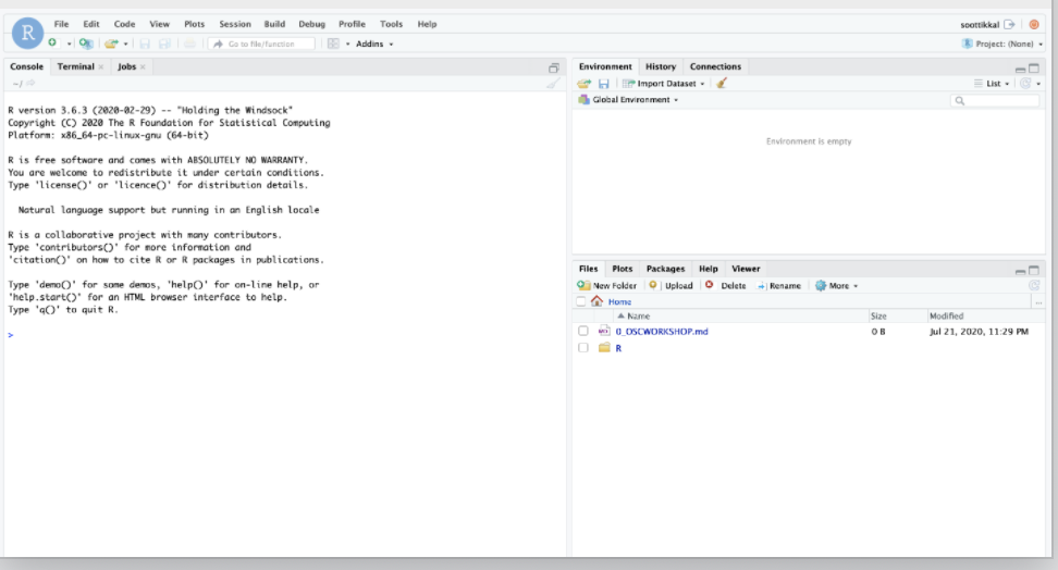
You can quit a Rstudio session by clicking on File from the top tabs then on the Quit. This will only quit the session, but the resource you requested is still held until walltime limit is reached. To release the resource, please click on DELETE in the Rstudio launch page.
Shared Access
PI can store and share materials like data, scripts, etc, and R packages with the class. We will set up a project space for the project ID of the course. This project space will be created under /fs/ess/project_ID. Once the project space is ready, please login to Owens or Pitzer as PI account of the classroom project. Run the following script with the project ID and course ID. This will create a folder with the course_ID under the project space and then two subfolders 1) Rpkgs 2) materials under it.
~support/classroom/tools/setup_rstudio_classroom /fs/ess/project_ID course_ID
Shared R packages
Once the class module is ready, PI can access the course at class.osc.edu under the Rstudio job submission page. PI can launch the course environment and install R packages for the class.
It is important to install R packages for the class only in the class R environment after launching the Rstudio interface for the course. If you install R packages without launching class Rstudio, R will have access to your personnel R libraries at $HOME and could affect the installation process.
After launching Rstudio, please run the .libPaths() as follows
> .libPaths()
[1] "/users/PZS0680/soottikkal/osc_classes/OSCWORKSHOP/R" "/fs/ess/PZS0687/OSCWORKSHOP/Rpkgs"
[3] "/usr/local/R/gnu/9.1/3.6.3/site/pkgs"                "/usr/local/R/gnu/9.1/3.6.3/lib64/R/library"
Here you will see four R library paths. The last two are system R library paths and are accessible for all OSC users. OSC installs a number of popular R packages at the site location. You can check available packages with library() command. The first path is a personal R library of each user in the course environment and is not shared with students. The second lib path is accessible to all students of the course(Eg: /fs/ess/PZS0687/OSCWORKSHOP/Rpkgs). PI should install R packages in this library to share with the class. As a precaution, it is a good idea to eliminate PI's personal R library from .libPaths() before R package installation as follows. Please note that this step is needed to be done only when preparing course materials by PI.
> .libPaths(.libPaths()[-1])
> .libPaths()
[1] "/fs/ess/PZS0687/OSCWORKSHOP/Rpkgs"          "/usr/local/R/gnu/9.1/3.6.3/site/pkgs"
[3] "/usr/local/R/gnu/9.1/3.6.3/lib64/R/library"
Now there is only one writable R library path such that all packages will be installed into this library path and shared for all users.
PI can install all packages required for the class using install.packages() function. Once the installation is complete, students will have access to all those packages.
Please note that students can also install their own packages. Those packages will be installed into their personable library in the class environment i.e., the first path listed under .libPaths()
Shared materials
PI can share materials like data, scripts, and rmd files stored in /fs/ess/project_ID/course_ID/materials with students. When a student launch a Rstduio session, the directory will be copied to the student's workspace $HOME/osc_classes/courseID (destination). Please inform us if you want to use a source directory other than /fs/ess/project_ID/course_ID/materials. The student will see the directory materials on the landing page. PI can add files to the material source directory. New files will be copied to the destination every time when a new Rstudio session starts. But If PI modifies existing files, the changes won't be copied as the files were copied before. Therefore we recommend renaming the file after the update so that it will be copied.
There are several different ways to copy materials manually from a directory to students' workspace. T
- On
class.osc.eduserver, click onFilesfrom the top tabs, then on$HOMEdirectory. From the top right, click onGo toand enter the storage path (Eg:/fs/ess/PZS0687/) in the box and press OK. This will open up storage path and users can copy files. Open the class folder from the$HOMEtree shown on left and paste files there. All files copied to$HOME/osc_classes/course_IDwill appear in the Rstudio FIle browser.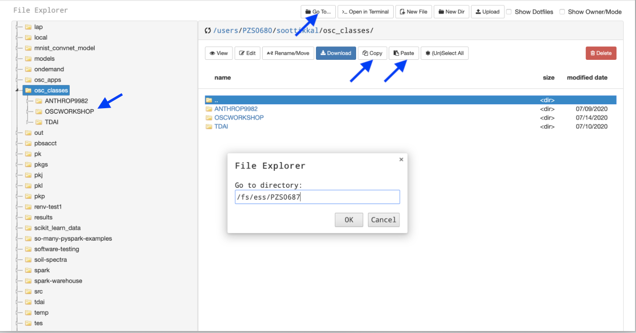
- On
class.osc.eduserver, Click onClustersfrom the top tabs, then onOwens Shell Access. This will open up a terminal on Owens where students can enter Unix command for copying. Eg:cp -r /fs/ess/PZS0687/OSCWORKSHOP/materials $HOME/osc_classes/course_ID
Please note that$HOME/osc_classes/course_IDwill be created only after launching Rstudio instance at least once. - Students can also upload material directly to Rstudio using the
uploadtab located in theFile browserof Rstudio from their local computer. This assumes they have already downloaded materials to their computers.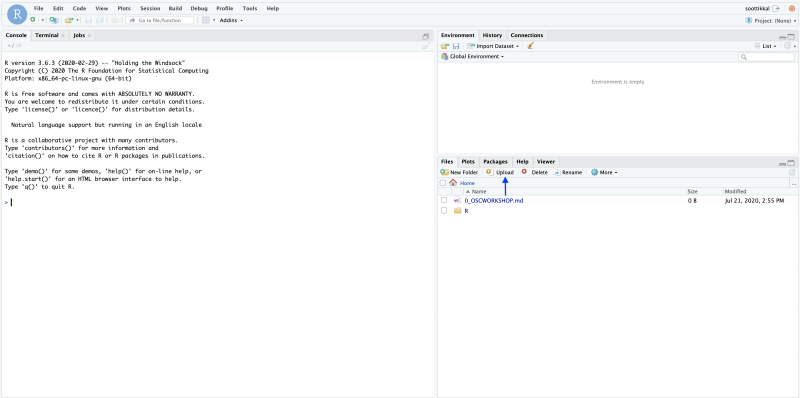
Checklist for PIs
- Apply for a classroom project ID that is unique to the course
- Add yourself, PI, to the project as an authorized user.
- Inform us about additional requirements such as R version or other software
- Once the class module is ready, create class materials under the storage path, and install R packages in the class environment.
- Make a reservation on OSC cluster for the class schedule.
- Invite students to the project at my.osc.edu to give them access to the project ID.
Please reach out to oschelp@osc.edu if you have any questions.
Using nbgrader for Classroom
Using ngbrader in Jupyter
Install nbgrader
You can install nbgrader in a notebook:
- Launch a Juypter session from class.osc.edu
- Open a new notebook
- To Install nbgrader, run:
!pip install nbgrader
!jupyter nbextension install --sys-prefix --py nbgrader --overwrite
!jupyter nbextension enable --sys-prefix --py nbgrader
!jupyter serverextension enable --sys-prefix --py nbgrader
To check the installed extensions, run
!jupyter nbextension list
There are six enabled extensions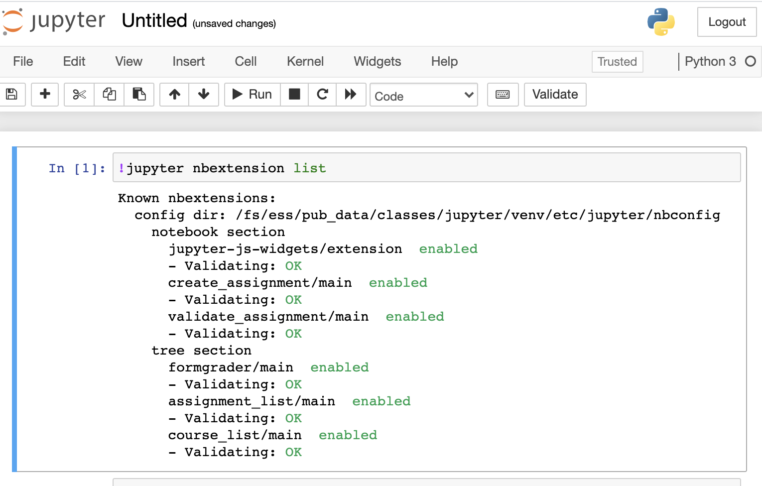
Configure nbgrader
In order to upload and collect assignments, nbgrader requires a exchange directory with write permissions for everyone. For example, to create a directory in project space, run:
%%bash
mkdir -p /fs/ess/projectID/courseID/exchange
chmod a+wx /fs/ess/projectID/courseID/exchange
Then get your cousre ID for configuratin. In a notebook, run:
%%bash
echo $OSC_CLASS_ID
Finally create the nbgrader configuration at the root of the workspace. In a notebook, run
%%file nbgrader_config.py
c = get_config()
c.CourseDirectory.course_id = "courseID"     # it must be the value of $OSC_CLASS_ID
c.Exchange.root = "/fs/ess/projectID/courseID/exchange"
c.Exchange.timezone = 'EST'
Once the file is created, you can launch a new Jupyter session then start creating assignments. For using nbgrader, please refer the nbgrader documents.
Access assignments
To let students access the assignments, students need to have the following configuration file in the root of their workspace:
%%file nbgrader_config.py
c = get_config()
c.Exchange.root = "/fs/ess/projectID/courseID/exchange"
HOWTO
Our HOWTO collection contains short tutorials that help you step through some of the common (but potentially confusing) tasks users may need to accomplish, that do not quite rise to the level of requiring more structured training materials. Items here may explain a procedure to follow, or present a "best practices" formula that we think may be helpful.
Service:
HOW TO: Look at requested time accuracy using XDMoD
The XDMoD tool at xdmod.osc.edu can be used to get an overview of how accurate the requested time of jobs are with the elapsed time of jobs.
One way of specifying a time request is:
#SBATCH --time=xx:xx:xx
The elapsed time is how long the job ran for before completing. This can be obtained using the sacct command.
$ sacct -u <username> --format=jobid,account,elapsed
It is important to understand that the requested time is used when scheduling a submitted job. If a job requests a time that is much more than the expected elapsed time, then it may take longer to start because the resources need to be allocated for the time that the job requests even if the job only uses a small portion of that requested time.
This allows one to view the requested time accuracy for an individual job, but XDMoD can be used to do this for jobs submitted in over a time range.
First, login to xdmod.osc.edu, see this page for more instructions.
https://www.osc.edu/supercomputing/knowledge-base/xdmod_tool
Then, navigate to the Metric Explorer tab.
Look for the Metric Catalog on the left side of the page and expand the SUPREMM options. Select Wall Hours: Requested: Per Job and group by None.
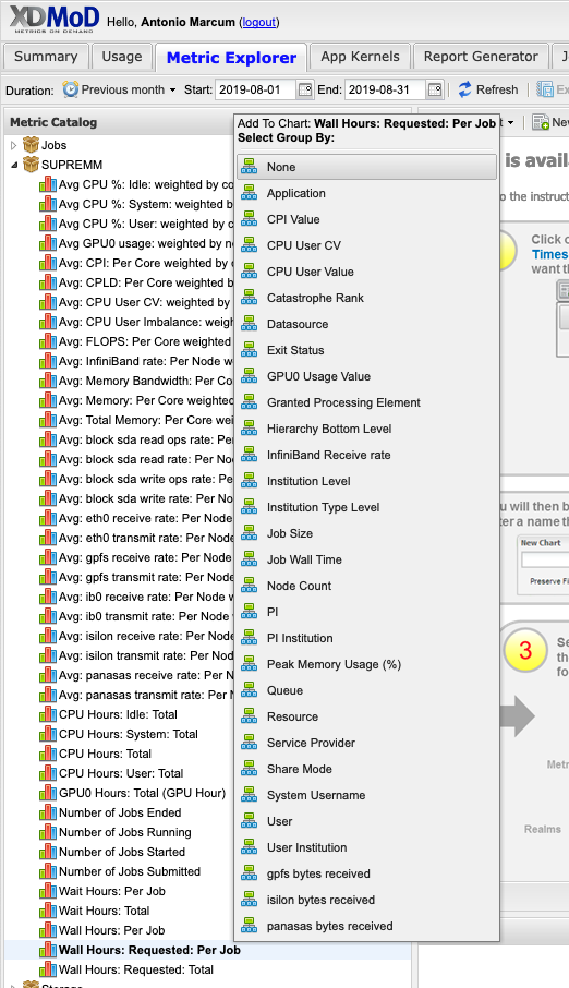
This will now show the average time requested.
The actual time data can be added by navigating to Add Data -> SUPREMM -> Wall Hours: Per Job.
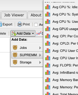

This will open a new window titled Data Series Definition, to change some parameters before showing the new data. In order to easily distinguish between elapsed and requested time, change the Display Type to Bar, then click add to view the new data.
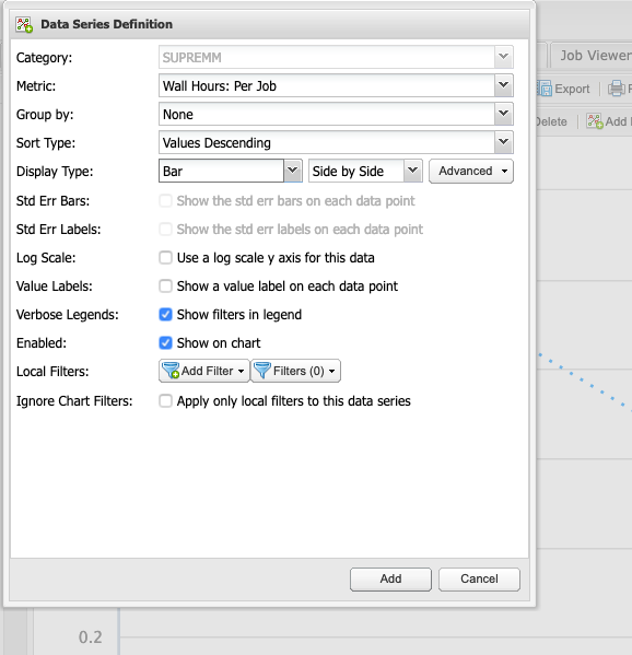
Now there is a line which shows the average requested time of jobs, and bars which depict the average elapsed time of jobs. Essentialy, the closer the bar is to the line, without intersecting the line, the more accurate the time predicition. If the bar intersects the line, then it may indicate the there was not enough time requested for a job to complete, but remember that these values are averages.
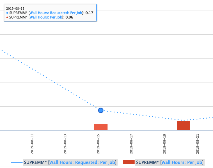
One can also view more detailed information about these jobs by clicking a data point and using the Show raw data option.
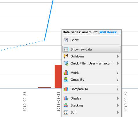
In order to have the Show raw data option, one may need to use the Drilldown option first to sort the jobs in that list by use or another metric.
HOWTO: Collect performance data for your program
This page outlines ways to generate and view performance data for your program using tools available at OSC.
Intel Tools
This section describes how to use performance tools from Intel. Make sure that you have an Intel module loaded to use these tools.
Intel VTune
Intel VTune is a tool to generate profile data for your application. Generating profile data with Intel VTune typically involves three steps:
1. Prepare the executable for profiling.
You need executables with debugging information to view source code line detail: re-compile your code with a -g option added among the other appropriate compiler options. For example:
mpicc wave.c -o wave -g -O3
2. Run your code to produce the profile data.
Profiles are normally generated in a batch job. To generate a VTune profile for an MPI program:
mpiexec <mpi args> amplxe-cl <vtune args> <program> <program args>
where <mpi args> represents arguments to be passed to mpiexec, <program> is the executable to be run, <vtune args> represents arguments to be passed to the VTune executable amplxe-cl, and <program args> represents arguments passed to your program.
For example, if you normally run your program with mpiexec -n 12 wave_c, you would use
mpiexec -n 12 amplxe-cl -collect hotspots -result-dir r001hs wave_c
To profile a non-MPI program:
amplxe-cl <vtune args> <program> <program args>
The profile data is saved in a .map file in your current directory.
As a result of this step, a subdirectory that contains the profile data files is created in your current directory. The subdirectory name is based on the -result-dir argument and the node id, for example, r001hs.o0674.ten.osc.edu.
3. Analyze your profile data.
You can open the profile data using the VTune GUI in interactive mode. For example:
amplxe-gui r001hs.o0674.ten.osc.edu
One should use an OnDemand VDI (Virtual Desktop Interface) or have X11 forwarding enabled (see Setting up X Windows). Note that X11 forwarding can be distractingly slow for interactive applications.
Intel ITAC
Intel Trace Analyzer and Collector (ITAC) is a tool to generate trace data for your application. Generating trace data with Intel ITAC typically involves three steps:
1. Prepare the executable for tracing.
You need to compile your executbale with -tcollect option added among the other appropriate compiler options to insert instrumentation probes calling the ITAC API. For example:
mpicc wave.c -o wave -tcollect -O3
2. Run your code to produce the trace data.
mpiexec -trace <mpi args> <program> <program args>
For example, if you normally run your program with mpiexec -n 12 wave_c, you would use
mpiexec -trace -n 12 wave_c
As a result of this step, .anc, .f, .msg, .dcl, .stf, and .proc files will be generated in your current directory.
3. Analyze the trace data files using Trace Analyzer
You will need to use traceanalyzer to view the trace data. To open Trace Analyzer:
traceanalyzer /path/to/<stf file>
where the base name of the .stf file will be the name of your executable.
One should use an OnDemand VDI (Virtual Desktop Interface) or have X11 forwarding enabled (see Setting up X Windows) to view the trace data. Note that X11 forwarding can be distractingly slow for interactive applications.
Intel APS
Intel's Application Performance Snapshot (APS) is a tool that provides a summary of your application's performance . Profiling HPC software with Intel APS typically involves four steps:
1. Prepare the executable for profiling.
Regular executables can be profiled with Intel APS. but source code line detail will not be available. You need executables with debugging information to view source code line detail: re-compile your code with a -g option added among the other approriate compiler options. For example:
mpicc wave.c -o wave -tcollect -O3
2. Run your code to produce the profile data directory.
Profiles are normally generated in a batch job. To generate profile data for an MPI program:
mpiexec -trace <mpi args> <program> <program args>
where <mpi args> represents arguments to be passed to mpiexec, <program> is the executable to be run and <program args> represents arguments passed to your program.
For example, if you normally run your program with mpiexec -n 12 wave_c, you would use
mpiexec -n 12 wave_c
To profile a non-MPI program:
aps <program> <program args>
The profile data is saved in a subdirectory in your current directory. The directory name is based on the date and time, for example, aps_result_YYYYMMDD/.
3. Generate the profile file from the directory.
To generate the html profile file from the result subdirectory:
aps --report=./aps_result_YYYYMMDD
to create the file aps_report_YYYYMMDD_HHMMSS.html.
4. Analyze the profile data file.
You can open the profile data file using a web browswer on your local desktop computer. This option typically offers the best performance.
ARM Tools
This section describes how to use performance tools from ARM.
ARM MAP
Instructions for how to use MAP is available here.
ARM DDT
Instructions for how to use DDT is available here.
ARM Performance Reports
Instructions for how to use Performance Reports is available here.
Other Tools
This section describes how to use other performance tools.
HPC Toolkit
Rice University's HPC Toolkit is a collection of performance tools. Instructions for how to use it at OSC is available here.
TAU Commander
TAU Commander is a user interface for University of Oregon's TAU Performance System. Instructions for how to use it at OSC is available here.
Service:
HOWTO: Create and Manage Python Environments
While our Python installations come with many popular packages installed, you may come upon a case in which you need an additional package that is not installed. If the specific package you are looking for is available from anaconda.org (formerlly binstar.org), you can easily install it and required dependencies by using the conda package manager.
Procedure
The following steps are an example of how to set up a Python environment and install packages to a local directory using conda. We use the name local for the environment, but you may use any other name.
Load proper Python module
We have python and Miniconda3 modules. python and miniconda3 module is based on Conda package manager. python modules are typically recommended when you use Python in a standard environment that we provide. However, if you want to create your own python environment, we recommend using miniconda3 module, since you can start with minimal configurations.
module load miniconda3
Create Python installation to local directory
Three alternative create commands are listed. These cover the most common cases.
CREATE NEW ENVIRONMENT
The following will create a minimal Python installation without any extraneous packages:
conda create -n local
CLONE BASE ENVIRONMENT
If you want to clone the full base Python environment from the system, you may use the following create command:
conda create -n local --clone base
CREATE NEW ENVIRONMENT WITH SPECIFIC PACKAGES
You can augment the command above by listing specific packages you would like installed into the environment. For example, the following will create a minimal Python installation with only the specified packages (in this case, numpy and babel):
conda create -n local numpy babel
By default, conda will install the newest versions of the packages it can find. Specific versions can be specified by adding =<version> after the package name. For example, the following will create a Python installation with Python version 2.7 and NumPy version 1.16:
conda create -n local python=2.7 numpy=1.16
CREATE NEW ENVIRONMENT WITH A SPECIFIC location
By default, conda will create the environment in your home location $HOME. To specify a location where the local environment is created, for example, in the project space /fs/ess/ProjectID, you can use the following command:
conda create --prefix /fs/ess/ProjectID/local
To activate the environment, use the command:
source activate /fs/ess/ProjectID/local
To verify that a clone has been created, use the command
conda info -e
For additional conda command documentation see https://docs.conda.io/projects/conda/en/latest/commands.html#conda-general-commands
Activate environment
Before the created environment can be used, it must be activated.
For the bash shell:
source activate local
At the end of the conda create step, you may saw a message from the installer that you can use conda activate command for activating environment. But, please don't use conda activate command, because it will try to update your shell configuration file and it may cause other issues. So, please use source activate command as we suggest above.
If you've previously utilized
conda init to enable the conda activate command, your shell configuration file such as .bashrc would have been altered with conda-specific lines. Upon activation of your environment using source activate, you may notice that the source activate/deactivate commands cease to function. However, we will be updating miniconda3 modules by May 15th 2024 to ensure that conda activate no longer alters the .bashrc file. Consequently, you can safely remove the conda-related lines between # >>> conda initialize >>> and # <<< conda initialize <<< from your .bashrc file and continue using the conda activate command.On newer versions of Anaconda on the Owens cluster you may also need to perform the removal of the following packages before trying to install your specific packages:
conda remove conda-build
conda remove conda-env
Install packages
To install additional packages, use the conda install command. For example, to install the yt package:
conda install yt
By default, conda will install the newest version if the package that it can find. Specific versions can be specified by adding =<version> after the package name. For example, to install version 1.16 of the NumPy package:
conda install numpy=1.16
If you need to install packages with pip, then you can install pip in your virtual environment by
conda install pip
Then, you can install packages with pip as
pip install PACKAGE
Please make sure that you have installed pip in your enviroment not using one from the miniconda module. The pip from the miniconda module will give access to the pacakges from the module to your environemt which may or may not be desired. Also set export PYTHONNOUSERSITE=True to prevent packages from user's .local path.
Test Python package
Now we will test our installed Python package by loading it in Python and checking its location to ensure we are using the correct version. For example, to test that NumPy is installed correctly, run
python -c "from __future__ import print_function; import numpy; print(numpy.__file__)"
and verify that the output generally matches
$HOME/.conda/envs/local/lib/python3.6/site-packages/numpy/__init__.py
To test installations of other packages, replace all instances of numpy with the name of the package you installed.
Remember, you will need to load the proper version of Python before you go to use your newly installed package. Packages are only installed to one version of Python.
Install your own Python packages
If the method using conda above is not working, or if you prefer, you can consider installing Python packages from the source. Please read HOWTO: install your own Python packages.
But I use virtualenv and/or pip!
See the comparison to these package management tools here:
https://docs.conda.io/projects/conda/en/latest/commands.html#conda-vs-pip-vs-virtualenv-commands
Use pip only without conda package manager
pip installations are supported:
module load python
module list                            # check which python you just loaded
pip install --user --upgrade PACKAGE   # where PACKAGE is a valid package name
Note the default installation prefix is set to the system path where OSC users cannot install the package. With the option --user, the prefix is set to $HOME/.local where lib, bin, and other top-level folders for the installed packages are placed. Finally, the option --upgrade will upgrade the existing packages to the newest available version.
The one issue with this approach is portability with multiple Python modules. If you plan to stick with a single Python module, then this should not be an issue. However, if you commonly switch between different Python versions, then be aware of the potential trouble in using the same installation location for all Python versions.
Use pip in a Python virtual environment (Python 3 only)
Typically, you can install packages with the methods shown in Install packages section above, but in some cases where the conda package installations have no source from conda channels or have dependency issues, you may consider using pip in an isolated Python virtual environment.
To create an isolated virtual environment:
module reset
python3 -m venv --without-pip $HOME/venv/mytest --prompt "local"
source $HOME/venv/mytest/bin/activate
(local) curl https://bootstrap.pypa.io/get-pip.py |python     # get the newest version of pip
(local) deactivate
where we use the path $HOME/venv/mytest and the name local for the environment, but you may use any other path and name.
To activate and deactivate the virtual environment:
source $HOME/venv/mytest/bin/activate
(local) deactivate
To install packages:
source $HOME/venv/mytest/bin/activate
(local) pip install PACKAGE
You don't need the --user option within the virtual environment.
Further Reading
Conda Test Drive: https://conda.io/docs/test-drive.html
HOWTO: Install Tensorflow locally
This documentation describes how to install tensorflow package locally in your $HOME space. For more details on Tensorflow see the software page.
Load python module
module load miniconda3/4.10.3-py37
We already provide some versions of tensorflow centrally installed on our clusters. To see the available versions, run conda list tensorflow. See software page for software details and usage instructions on the clusters.
If you need to install tensorflow versions not already provided or would like to use tensorflow in a conda environment proceed with the tutorial below.
Create Python Environment
First we will create a conda environment which we will later install tensorflow into. See HOWTO: Create and Manage Python Environments for details on how to create and setup your environemnt.
Make sure you activate your environment before proceeding:
source activate MY_ENV
Install package
Install the latest version of tensorflow.
conda install tensorflow
You can see all available version for download on conda with conda search tensorflow
There is also a gpu compatable version called tensorflow-gpu
If there are errors on this step you will need to resolve them before continuing.
Test python package
Now we will test tensorflow package by loading it in python and checking its location to ensure we are using the correct version.
python -c "import tensorflow;print (tensorflow.__file__)"
Output:
$HOME/.conda/envs/MY_ENV/lib/python3.9/site-packages/tensorflow/__init__.py
Remember, you will need to load the proper version of python before you go to use your newly installed package. Packages are only installed to one version of python.
Please refer HOWTO: Use GPU with Tensorflow and PyTorch if you would like to use tenorflow with Gpus.
Supercomputer:
HOWTO: Install Python packages from source
While we provide a number of Python packages, you may need a package we do not provide. If it is a commonly used package or one that is particularly difficult to compile, you can contact OSC Help for assistance. We also have provided an example below showing how to build and install your own Python packages and make them available inside of Python. These instructions use "bash" shell syntax, which is our default shell. If you are using something else (csh, tcsh, etc), some of the syntax may be different.
Please consider using conda Python package manager before you try to build Python using the method explained here. We have instructions on conda here.
Gather your materials
First, you need to collect what you need in order to perform the installation. We will do all of our work in $HOME/local/src. You should make this directory now.
mkdir -p $HOME/local/src
Next, we will need to download the source code for the package we want to install. In our example, we will use NumExpr. (NumExpr is already available through conda, so it is recommended you use conda to install it: tutorial here. The following steps are simply an example of the procedure you would follow to perform an installation of software unavailable in conda or pip). You can either download the file to your desktop and then upload it to OSC, or directly download it using the wget utility (if you know the URL for the file).
cd ~/local/src
wget https://github.com/pydata/numexpr/releases/download/v2.8.4/numexpr-2.8.4.tar.gz
Next, extract the downloaded file. In this case, since it's a "tar.gz" format, we can use tar to decompress and extract the contents.
tar xvfz numexpr-2.8.4.tar.gz
You can delete the downloaded archive now or keep it should you want to start the installation from scratch.
Build it!
Environment
To build the package, we will want to first create a temporary environment variable to aid in installation. We'll call INSTALL_DIR.
export INSTALL_DIR=${HOME}/local/numexpr/2.8.4
We are roughly following the convention we use at the system level. This allows us to easily install new versions of software without risking breaking anything that uses older versions. We have specified a folder for the program (numexpr), and for the version (2.8.4). To be consistent with Python installations, we will create a second temporary environment variable that will contain the actual installation location.
export TREE=${INSTALL_DIR}/lib/python3.6/site-packages
Next, make the directory tree.
mkdir -p $TREE
Compile
To compile the package, we should switch to the GNU compilers. The system installation of Python was compiled with the GNU compilers, and this will help avoid any unnecessary complications. We will also load the Python package, if it hasn't already been loaded.
module swap intel gnu
module load python/3.6-conda5.2
Next, build it. This step may vary a bit, depending on the package you are compiling. You can execute python setup.py --help to see what options are available. Since we are overriding the install path to one that we can write to and that fits our management plan, we need to use the --prefix option.
NumExpr build also requires us to set the PYTHONPATH variable before building:
export PYTHONPATH=$PYTHONPATH:~/local/numexpr/2.8.4/lib/python3.6/site-packages
Find the setup.py file:
cd numexpr-2.8.4
Now to build:
python setup.py install --prefix=$INSTALL_DIR
Make it usable
At this point, the package is compiled and installed in ~/local/numexpr/2.8.4/lib/python3.6/site-packages. Occasionally, some files will be installed in ~/local/numexpr/2.8.4/bin as well. To ensure Python can locate these files, we need to modify our environment.
Manual
The most immediate way -- but the one that must be repeated every time you wish to use the package -- is to manually modify your environment. If files are installed in the "bin" directory, you'll need to add it to your path. As before, these examples are for bash, and may have to be modified for other shells. Also, you will have to modify the directories to match your install location.
export PATH=$PATH:~/local/numexpr/2.8.4/bin
And for the Python libraries:
export PYTHONPATH=$PYTHONPATH:~/local/numexpr/2.8.4/lib/python3.6/site-packages
Hardcode it
We don't recommend this option, as it is less flexible and can cause conflicts with system software. But if you want, you can modify your .bashrc (or similar file, depending on your shell) to set these environment variables automatically. Be extra careful; making a mistake in .bashrc (or similar) can destroy your login environment in a way that will require a system administrator to fix. To do this, you can copy the lines above modifying $PATH and $PYTHONPATH into .bashrc. Remember to test them interactively first. If you destroy your shell interactively, the fix is as simple as logging out and then logging back in. If you break your login environment, you'll have to get our help to fix it.
Make a module (recommended!)
This is the most complicated option, but it is also the most flexible, as you can have multiple versions of this particular software installed and specify at run-time which one to use. This is incredibly useful if a major feature changes that would break old code, for example. You can see our tutorial on writing modules here, but the important variables to modify are, again, $PATH and $PYTHONPATH. You should specify the complete path to your home directory here and not rely on any shortcuts like ~ or $HOME. Below is a modulefile written in Lua:
If you are following the tutorial on writing modules, you will want to place this file in $HOME/local/share/lmodfiles/numexpr/2.8.4.lua:
-- This is a Lua modulefile, this file 2.8.4.lua can be located anywhere
-- But if you are following a local modulefile location convention, we place them in
-- $HOME/local/share/lmodfiles/
-- For numexpr we place it in $HOME/local/share/lmodfiles/numexpr/2.8.4.lua
-- This finds your home directory
local homedir = os.getenv("HOME")
prepend_path("PYTHONPATH",
pathJoin(homedir, "/local/numexpr/2.8.4/lib/python3.6/site-packages"))
prepend_path(homedir, "local/numexpr/2.8.4/bin")
Once your module is created (again, see the guide), you can use your Python package simply by loading the software module you created.
module use $HOME/local/share/lmodfiles/
module load numexpr/2.8.4
Service:
HOWTO: Use GPU with Tensorflow and PyTorch
GPU Usage on Tensorflow
Environment Setup
To begin, you need to first create and new conda environment or use an already existing one. See HOWTO: Create Python Environment for more details. In this example we are using python/3.6-conda5.2
Once you have a conda environment created and activated we will now install tensorflow-gpu into the environment (In this example we will be using version 2.4.1 of tensorflow-gpu:
conda install tensorflow-gpu=2.4.1
Verify GPU accessability (Optional):
Now that we have the environment set up we can check if tensorflow can access the gpus.
To test the gpu access we will submit the following job onto a compute node with a gpu:
#!/bin/bash
#SBATCH --account <Project-Id>
#SBATCH --job-name Python_ExampleJob
#SBATCH --nodes=1
#SBATCH --time=00:10:00
#SBATCH --gpus-per-node=1


module load python/3.6-conda5.2 cuda/11.8.0

source activate tensorflow_env


# run either of the following commands

python << EOF
import tensorflow as tf
print(tf.test.is_built_with_cuda())
EOF

python << EOF
from tensorflow.python.client import device_lib
print(device_lib.list_local_devices())
EOF
You will know tensorflow is able to successfully access the gpu if tf.test.is_built_with_cuda() returns True and device_lib.list_local_devices() returns an object with /device:GPU:0 as a listed device.
At this point tensorflow-gpu should be setup to utilize a GPU for its computations.
GPU vs CPU
A GPU can provide signifcant performace imporvements to many machine learnings models. Here is an example python script demonstrating the performace improvements. This is ran on the same environment created in the above section.
from timeit import default_timer as timer
import tensorflow as tf
from tensorflow import keras
import numpy as np


(X_train, y_train), (X_test, y_test) = keras.datasets.cifar10.load_data()


# scaling image values between 0-1
X_train_scaled = X_train/255
X_test_scaled = X_test/255

# one hot encoding labels
y_train_encoded = keras.utils.to_categorical(y_train, num_classes = 10)
y_test_encoded = keras.utils.to_categorical(y_test, num_classes = 10)

def get_model():
    model = keras.Sequential([
        keras.layers.Flatten(input_shape=(32,32,3)),
        keras.layers.Dense(3000, activation='relu'),
        keras.layers.Dense(1000, activation='relu'),
        keras.layers.Dense(10, activation='sigmoid')
    ])

    model.compile(optimizer='SGD',
              loss='categorical_crossentropy',
              metrics=['accuracy'])
    return model

# GPU
with tf.device('/GPU:0'):
    start = timer()
    model_cpu = get_model()
    model_cpu.fit(X_train_scaled, y_train_encoded, epochs = 1)
    end = timer()


print("GPU time: ", end - start)

# CPU
with tf.device('/CPU:0'):
    start = timer()
    model_gpu = get_model()
    model_gpu.fit(X_train_scaled, y_train_encoded, epochs = 1)
    end = timer()

print("CPU time: ", end - start)
Example code sampled from here
The above code was then submitted in a job with the following script:
#!/bin/bash
#SBATCH --account <Project-Id>
#SBATCH --job-name Python_ExampleJob
#SBATCH --nodes=1
#SBATCH --time=00:10:00
#SBATCH --gpus-per-node=1

module load python/3.6-conda5.2 cuda/11.8.0

source activate tensorflow_env

python tensorflow_example.py
Make sure you request a gpu! For more information see GPU Computing
As we can see from the output, the GPU provided a signifcant performace improvement.
GPU time:  3.7491355929996644

CPU time:  78.8043485119997
Usage on Jupyter
If you would like to use a gpu for your tensorflow project in a jupyter notebook follow the below commands to set up your environment.
To begin, you need to first create and new conda environment or use an already existing one. See HOWTO: Create Python Environment for more details. In this example we are using python/3.6-conda5.2
Once you have a conda environment created and activated we will now install tensorflow-gpu into the environment (In this example we will be using version 2.4.1 of tensorflow-gpu:
conda install tensorflow-gpu=2.4.1
Now we will setup a jupyter kernel. See HOWTO: Use a Conda/Virtual Environment With Jupyter for details on how to create a jupyter kernel with your conda environment.
Once you have the kernel created see Usage section of Python page for more details on accessing the Jupyter app from OnDemand.
When configuring your notebook make sure to select a GPU enabled node and a cuda version.
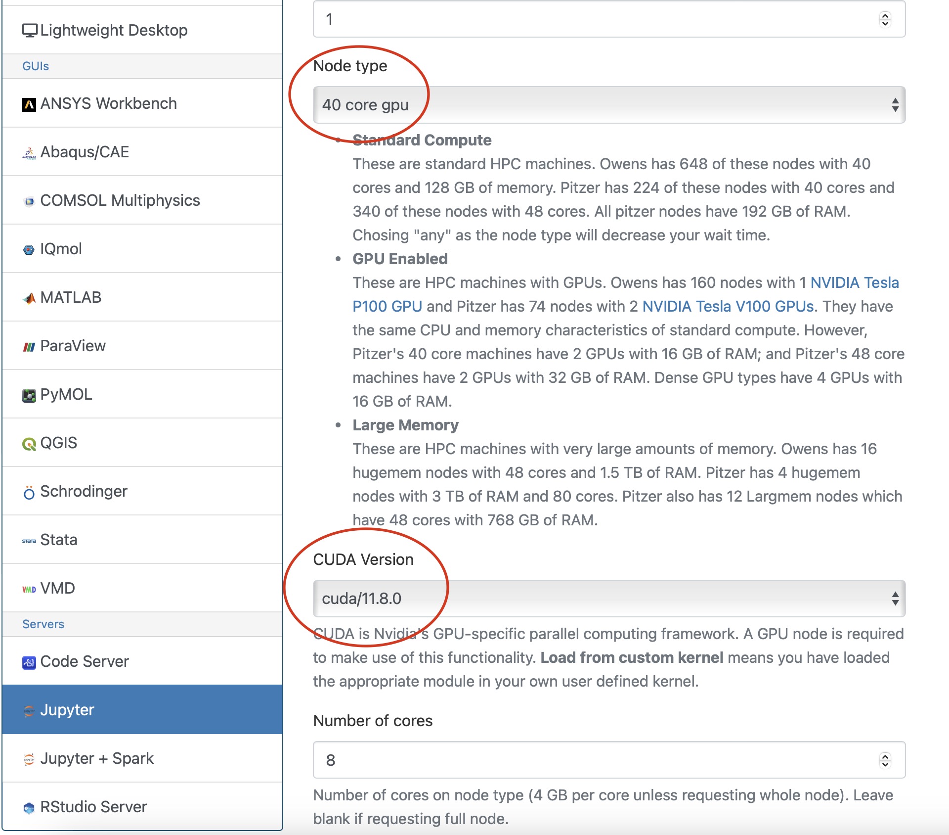
Now you are all setup to use a gpu with tensorflow on a juptyer notebook.
GPU Usage on PyTorch
Environment Setup
To begin, you need to first create and new conda environment or use an already existing one. See HOWTO: Create Python Environment for more details. In this example we are using python/3.6-conda5.2
Once you have a conda environment created and activated we will now install pytorch into the environment (In the example we will be using version 1.3.1 of pytorch:
conda install pytorch=1.3.1
Verify GPU accessability (Optional):
Now that we have the environment set up we can check if pytorch can access the gpus.
To test the gpu access we will submit the following job onto a compute node with a gpu:
#!/bin/bash
#SBATCH --account <Project-Id>
#SBATCH --job-name Python_ExampleJob
#SBATCH --nodes=1
#SBATCH --time=00:10:00
#SBATCH --gpus-per-node=1


ml python/3.6-conda5.2 cuda/11.8.0

source activate pytorch_env


python << EOF
import torch
print(torch.cuda.is_available())
device = torch.device("cuda:0" if torch.cuda.is_available() else "cpu")
print(device)
EOF
You will know pytorch is able to successfully access the gpu if torch.cuda.is_available() returns True and torch.device("cuda:0" if torch.cuda.is_available() else "cpu") returns cuda:0 .
At this point PyTorch should be setup to utilize a GPU for its computations.
GPU vs CPU
Here is an example pytorch script demonstrating the performace improvements from GPUs
import torch
from timeit import default_timer as timer


# check for cuda availability
print("Cuda: ", torch.cuda.is_available())
device = torch.device("cuda:0" if torch.cuda.is_available() else "cpu")
print("Device: ", device)


#GPU
b = torch.ones(4000,4000).cuda() # Create matrix on GPU memory
start_time = timer()
for _ in range(1000):
    b += b
elapsed_time = timer() - start_time

print('GPU time = ',elapsed_time)


#CPU
a = torch.ones(4000,4000) # Create matrix on CPU memory
start_time = timer()
for _ in range(1000):
    a += a
elapsed_time = timer() - start_time

print('CPU time = ',elapsed_time)
The above code was then submitted in a job with the following script:
#!/bin/bash
#SBATCH --account <Project-Id>
#SBATCH --job-name Python_ExampleJob
#SBATCH --nodes=1
#SBATCH --time=00:10:00
#SBATCH --gpus-per-node=1

ml python/3.6-conda5.2 cuda/11.8.0

source activate pytorch_env

python pytorch_example.py
Make sure you request a gpu! For more information see GPU Computing
As we can see from the output, the GPU provided a signifcant performace improvement.
GPU time =  0.0053490259997488465

CPU time =  4.232843188998231
Usage on Jupyter
If you would like to use a gpu for your PyTorch project in a jupyter notebook follow the below commands to set up your environment.
To begin, you need to first create and new conda environment or use an already existing one. See HOWTO: Create Python Environment for more details. In this example we are using python/3.6-conda5.2
Once you have a conda environment created and activated we will now install pytorch into the environment (In the example we will be using version 1.3.1 of pytorch:
conda install pytorch=1.3.1
You also may need to install numba for PyTorch to access a gpu from the jupter notebook.
conda install numba=0.54.1
Now we will setup a jupyter kernel. See HOWTO: Use a Conda/Virtual Environment With Jupyter for details on how to create a jupyter kernel with your conda environment.
Once you have the kernel created see Usage section of Python page for more details on accessing the Jupyter app from OnDemand.
When configuring your notebook make sure to select a GPU enabled node and a cuda version.
Now you are all setup to use a gpu with PyTorch on a juptyer notebook.
Horovod
If you are using Tensorflow or PyTorch you may want to also consider using Horovod. Horovod will take single-GPU training scripts and scale it to train across many GPUs in parallel.
HOWTO: Debugging Tips
This article focuses on debugging strategies for C/C++ codes, but many are applicable to other languages as well.
Rubber Duck Debugging
This approach is a great starting point. Say you have written some code, and it does not do what you expect it to do. You have stared at it for a few minutes, but you cannot seem to spot the problem.
Try explaining what the problem is to a rubber duck. Then, walk the rubber duck through your code, line by line, telling it what it does. Don’t have a rubber duck? Any inanimate object will do (or even an animate one if you can grab a friend).
It sounds silly, but rubber duck debugging helps you to get out of your head, and hopefully look at your code from a new perspective. Saying what your code does (or is supposed to do) out loud has a good chance of revealing where your understanding might not be as good as you think it is.
Printf() Debugging
You’ve written a whole bunch of new code. It takes some inputs, chugs along for a while, and then creates some outputs. Somewhere along this process, something goes wrong. You know this because the output is not at all what you expected. Unfortunately, you have no idea where things are going wrong in the code.
This might be a good time to try out printf() debugging. It’s as simple as its name implies: simply add (more) printf() statements to your code. You’ve likely seen this being used. It’s the name given to the infamous ‘printf(“here”);’ calls used to verify that a particular codepath is indeed taken.
Consider printing out arguments and return values to key functions. Or, the results or summary statistics from large calculations. These values can be used as “sanity checks” to ensure that up until that point in the code, everything is going as expected.
Assertion calls, such as "assert(...)", can also be used for a similar purpose. However, often the positive feedback you get from print statements is helpful in when you’re debugging. Seeing a valid result printed in standard out or a log file tells you positively that at least something is working correctly.
Debuggers
Debuggers are tools that can be used to interactively (or with scripts) debug your code. A fairly common debugger for C and C++ codes is gdb. Many guides exist online for using gdb with your code.
OSC systems also provide the ARM DDT debugger. This debugger is designed for use with HPC codes and is arguably easier to use than gdb. It can be used to debug MPI programs as well.
Debuggers allow you to interact with the program while it is running. You can do things like read and write variable values, or check to see if/when certain functions are called.
Testing
Okay, this one isn’t exactly a debugging strategy. It’s a method to catch bugs early, and even prevent the addition of bugs. Writing a test suite for your code that’s easy to run (and ideally fast) lets you test new changes to ensure they don’t break existing functionality.
There are lots of different philosophies on testing software. Too many to cover here. Here’s two concepts that are worth looking into: unit testing and system testing.
The idea behind unit testing is writing tests for small “units” of code. These are often functions or classes. If you know that the small pieces that make up your code work, then you’ll have more confidence in the overall assembled program. There’s an added architecture benefit here too. Writing code that is testable in the first place often results in code that’s broken up into separate logical pieces (google “separation of concerns”). This makes your code more modular and less “spaghetti-like”. Your code will be easier to modify and understand.
The second concept – system testing – involves writing tests that run your entire program. These often take longer than unit tests, but have the added benefit that they’ll let you know whether or not your entire program still works after introducing a new change.
When writing tests (both system and unit tests), it’s often helpful to include a couple different inputs. Occasionally a program may work just fine for one input, but fail horribly with another input.
Minimal, Reproducible Example
Maybe your code takes a couple hours (or longer…) to run. There’s a bug in it, but every time you try to fix it, you have to wait a few hours to see if the fix worked. This is driving you crazy.
A possible approach to make your life easier is to try to make a Minimal, Reproducible Example (see this stackoverflow page for information).
Try to extract just the code that fails, from your program, and also its inputs. Wrap this up into a separate program. This allows you to run just the code that failed, hopefully greatly reducing the time it takes to test out fixes to the problem.
Once you have this example, can you make it smaller? Maybe take out some code that’s not needed to reproduce the bug, or shrink the input even further? Doing this might help you solve the problem.
Tools and other resources
- Compiler warnings – compilers are your friend. Chances are your compiler has a flag that can be used to enable more warnings than are on by default. GNU tools have “-Wall” and “-Wextra”. These can be used to instruct the compiler to tell you about places in the code where bugs may exist.
- The Practice of Programming by Brian Kernighan and Rob Pike contains a very good chapter on debugging C and C++ programs.
- Valgrind is a tool that can be used for many types of debugging including looking for memory corruptions and leaks. However, it slows down your code a very sizeable amount. This might not be feasible for HPC codes
- ASAN (address sanitizer) is another tool that can be used for memory debugging. It is less featureful than Valgrind, but runs much quicker, and so will likely work with your HPC code.
Service:
HOWTO: Establish durable SSH connections
In December 2021 OSC updated its firewall to enhance security. As a result, SSH sessions are being closed more quickly than they used to be. It is very easy to modify your SSH options in the client you use to connect to OSC to keep your connection open.
In ~/.ssh/config (use the command touch ~/.ssh/config to create it if there is no exisitng one), you can set 3 options:
TCPKeepAlive=no
ServerAliveInterval=60
ServerAliveCountMax=5
Please refer to your SSH client documentation for how to set these options in your client.
Service:
HOWTO: Identify users on a project account and check status
An eligible principal investigator (PI) heads a project account and can authorize/remove user accounts under the project account (please check our Allocations and Accounts documentation for more details). This document shows you how to identify users on a project account and check the status of each user.
Identify Users on a Project Account
If you know the project acccount
If the project account (projectID) is known, the OSCgetent command will list all users on the project:
$ OSCgetent group projectID
The returned information is in the format of:
projectID:*:gid: list of user IDs
gid is the group identifier number unique for the project account projectID.
For example, the command OSCgetent group PZS0712 lists all users on the project account PZS0712 as below:
$ OSCgetent group PZS0712
PZS0712:*:5513:amarcum,guilfoos,hhamblin,kcahill,xwang
Multiple groups can also be queried at once.
For Example, the command OSCgetent group PZS0712 PZS0726 lists all users on both PZS0712 and PZS0726:
PZS0712:*:5513:amarcum,guilfoos,hhamblin,kcahill,xwang
PZS0726:*:6129:amarcum,kkappel
Details on a project can also be obtained along with the user list using the OSCfinger command.
$ OSCfinger -g projectID
This returns:
Group: projectID                                  GID: XXXX
Status: 'active/restricted/etc'                   Type: XX
Principal Investigator: 'PI email'                Admins: NA
Members: 'list of users'
Category: NA
Institution: 'affliated institution'
Description: 'short description'
---
If you don't know the project acccount, but know the username
If the project account is not known, but the username is known, use the OSCfinger command to list all of the groups the user belongs to:
OSCfinger username
The returned information is in the format of:
Login: username                                   Name: First Last
Directory: home directory path                    Shell: /bin/bash
E-mail: user's email address
Primary Group: user's primary project
Groups: list of projects and other groups user is in
Password Changed: date password was last changed  Password Expires: date password expires
Login Disabled: TRUE/FALSE                             Password Expired: TRUE/FALSE
Current Logins:
Displays if user is currently logged in and from where/when
For example, with the username as amarcum, the command OSCfinger amarcum returns the information as below:
$ OSCfinger amarcum
Login: amarcum                                    Name: Antonio Marcum
Directory: /users/PZS0712/amarcum                 Shell: /bin/bash
E-mail: amarcum@osc.edu
Primary Group: PZS0712
Groups: sts,ruby,l2supprt,oscall,clntstf,oscstaff,clntall,PZS0712,PZS0726
Password Changed: May 12 2019 15:47 (calculated)  Password Expires: Aug 11 2019 12:05 AM
Login Disabled: FALSE                             Password Expired: FALSE
Current Logins:
On since Mar 07 2019 12:12 on pts/14 from pitzer-login01.hpc.osc.edu
----
If you don't know either the project account or user account
If the project account or username is not known, use the OSCfinger -e command with the '-e' flag to get the user account based on the user's name.
Use the following command to list all of the user accounts associated with a First and Last name:
$ OSCfinger -e 'First Last'
For example, with user's first name as Summer and last name as Wang, the command
OSCfinger -e 'Summer Wang' returns the information as below:
$ OSCfinger -e 'Summer Wang'
Login: xwang                                      Name: Summer Wang
Directory: /users/oscgen/xwang                    Shell: /bin/bash
E-mail: xwang@osc.edu
Primary Group: PZS0712
Groups: amber,abaqus,GaussC,comsol,foampro,sts,awsmdev,awesim,ruby,matlab,aasheats,mars,ansysflu,wrigley,lgfuel,l2supprt,fsl,oscall,clntstf,oscstaff,singadm,clntall,dhgremot,fsurfer,PZS0530,PCON0003,PZS0680,PMIU0149,PZS0712,PAS1448
Password Changed: Jan 08 2019 11:41               Password Expires: Jul 08 2019 12:05 AM
Login Disabled: FALSE                             Password Expired: FALSE
---
Once you know the user account username, follow the discussions in the previous section identify users on a project to get all user accounts on the project. Please contact OSC Help if you have any questions.
Check the Status of a User
Use the OSCfinger command to check the status of a user account as below:
OSCfinger username
For example, if the username is xwang, the command OSCfinger xwang will return:
$ OSCfinger xwang
Login: xwang                                      Name: Summer Wang
Directory: /users/oscgen/xwang                    Shell: /bin/bash
E-mail: xwang@osc.edu
Primary Group: PZS0712
Groups: amber,abaqus,GaussC,comsol,foampro,sts,awsmdev,awesim,ruby,matlab,aasheats,mars,ansysflu,wrigley,lgfuel,l2supprt,fsl,oscall,clntstf,oscstaff,singadm,clntall,dhgremot,fsurfer,PZS0530,PCON0003,PZS0680,PMIU0149,PZS0712,PAS1448
Password Changed: Jan 08 2019 11:41               Password Expires: Jul 08 2019 12:05 AM
Login Disabled: FALSE                             Password Expired: FALSE
---
- The home directory of xwang is
Directory: /users/oscgen/xwang - The shell of xwang is bash (
Shell: /bin/bash). If the information isShell:/access/denied, it means this user account has been either archived or restricted. Please contact OSC Help if you'd like to reactivate this user account. - xwang@osc.edu is the associated email with the user account xwang; that is, all OSC emails related to the account xwang will be sent to xwang@osc.edu (
Mail forwarded to xwang@osc.edu). Please contact OSC Help if the email address associated with this user account has been changed to ensure important notifications/messages/reminders from OSC may be received in a timely manner.
Check the Usage and Quota of a User's Home Directory/Project Space
All users see their file system usage statistics when logging in, like so:
As of 2018-01-25T04:02:23.749853 userid userID on /users/projectID used XGB of quota 500GB and Y files of quota 1000000 files
The information is from the file /users/reporting/storage/quota/*_quota.txt , which is updated twice a day. Some users may see multiple lines associated with a username, as well as information on project space usage and quota of their Primary project, if there is one. The usage and quota of the home directory of a username is provided by the line including the file server your home directory is on (for more information, please visit Home Directories), while others (generated due to file copy) can be safely ignored.
You can check any user's home directory or a project's project space usage and quota by running:
grep -h 'userID' OR 'projectID' /users/reporting/storage/quota/*_quota.txt
Here is an example of project PZS0712:
$ grep -h PZS0712 /users/reporting/storage/quota/*_quota.txt
As of 2019-03-07T13:55:01.000000 project/group PZS0712 on /fs/project used 262 GiB of quota 2048 GiB and 166987 files of quota 200000 files
As of 2019-03-07T13:55:01.000000 userid xwang on /fs/project/PZS0712 used 0 GiB of quota 0 GiB and 21 files of quota 0 files
As of 2019-03-07T13:55:01.000000 userid dheisterberg on /fs/project/PZS0712 used 262 GiB of quota 0 GiB and 166961 files of quota 0 files
As of 2019-03-07T13:55:01.000000 userid amarcum on /fs/project/PZS0712 used 0 GiB of quota 0 GiB and 2 files of quota 0 files
As of 2019-03-07T13:55:01.000000 userid root on /fs/project/PZS0712 used 0 GiB of quota 0 GiB and 2 files of quota 0 files
As of 2019-03-07T13:55:01.000000 userid guilfoos on /fs/project/PZS0712 used 0 GiB of quota 0 GiB and 1 files of quota 0 files
As of 2019-03-07T13:51:23.000000 userid amarcum on /users/PZS0712 used 399.86 MiB of quota 500 GiB and 8710 files of quota 1000000 files
Here is an example for username amarcum:
$ grep -h amarcum /users/reporting/storage/quota/*_quota.txt
As of 2019-03-07T13:55:01.000000 userid amarcum on /fs/project/PZS0712 used 0 GiB of quota 0 GiB and 2 files of quota 0 files
As of 2019-03-07T13:56:39.000000 userid amarcum on /users/PZS0645 used 4.00 KiB of quota 500 GiB and 1 files of quota 1000000 files
As of 2019-03-07T13:56:39.000000 userid amarcum on /users/PZS0712 used 399.86 MiB of quota 500 GiB and 8710 files of quota 1000000 files
Check the RU Usage for Projects and Users
The OSCusage commnad can provide detailed information about computational usage for a given project and user.
See the OSCusage command page for details.
Service:
HOWTO: Install a MATLAB toolbox
If you need to use a MATLAB toolbox that is not provided through our installations. You can follow these instructions, and if you have any difficulties you can contact OSC Help for assistance.
A reminder: It is your responsibility to verify that your use of software packages on OSC’s systems including any 3rd party toolboxes (whether installed by OSC staff or by yourself) complies with the packages’ license terms.
Gather your materials
First, we recommend making a new directory within your home directory in order to keep everything organized. You can use the unix command to make a new directory: "mkdir"
Now you can download the toolbox either to your desktop, and then upload it to OSC, or directly download it using the "wget" utility (if you know the URL for the file).
Now you can extract the downloaded file.
Adding the path
There are two methods on how to add the MATLAB toolbox path.
Method 1: Load up the Matlab GUI and click on "Set Path" and "Add folder"
Method 2: Use the "addpath" fuction in your script. More information on the function can be found here: https://www.mathworks.com/help/matlab/ref/addpath.html
Running the toolbox
Please refer to the instructions given alongside the toolbox. They should contain instructions on how to run the toolbox.
Service:
Technologies:
Fields of Science:
HOWTO: Install your own Perl modules
While we provide a number of Perl modules, you may need a module we do not provide. If it is a commonly used module, or one that is particularly difficult to compile, you can contact OSC Help for assistance, but we have provided an example below showing how to build and install your own Perl modules. Note, these instructions use "bash" shell syntax; this is our default shell, but if you are using something else (csh, tcsh, etc), some of the syntax may be different.
CPAN Minus
CPAN, the Comprehensive Perl Achive Network, is the primary source for publishing and fetching the latest modules and libraries for the Perl programming language. The default method for installing Perl modules using the "CPAN Shell", provides users with a great deal of power and flexibility but at the cost of a complex configuration and inelegant default setup.
Setting Up CPAN Minus
To use CPAN Minus with the system Perl (version 5.16.3), we need to ensure that the "cpanminus" module is loaded, if it hasn't been loaded already.
module load cpanminus
Please note that this step is not required if you have already loaded a version of Perl using the module load command.
Next, in order to use cpanminus, you will need to run the following command only ONCE:
perl -I $CPANMINUS_INC -Mlocal::lib
Using CPAN Minus
In most cases, using CPAN Minus to install modules is as simple as issuing a command in the following form:
cpanm [Module::Name]
For example, below are three examples of installing perl modules:
cpanm Math::CDF
cpanm SET::IntervalTree
cpanm DB_File
Testing Perl Modules
To test a perl module import, here are some examples below:
perl -e "require Math::CDF"
perl -e "require Set::IntervallTree"
perl -e "require DB_File"
The modules are installed correctly if no output is printed.
What Local Modules are Installed in my Account?
To show the local modules you have installed in your user account:
perldoc perllocal
Reseting Module Collection
If you should ever want to start over with your perl module collection, delete the following folders:
rm -r ~/perl5
rm -r ~/.cpanm
Service:
HOWTO: Locally Installing Software
Sometimes the best way to get access to a piece of software on the HPC systems is to install it yourself as a "local install". This document will walk you through the OSC-recommended procedure for maintaining local installs in your home directory or project space. The majority of this document describes the process of "manually" building and installing your software. We also show a partially automated approach through the use of a bash script in the Install Script section near the end.
NOTE: Throughout this document we'll assume you're installing into your home directory, but you can follow the steps below in any directory for which you have read/write permissions.
This document assumes you are familiar with the process of building software using "configure" or via editing makefiles, and only provides best practices for installing in your home directory.
Getting Started
Before installing your software, you should first prepare a place for it to live. We recommend the following directory structure, which you should create in the top-level of your home directory:
    local
    |-- src
    |-- share
        `-- lmodfiles
This structure is analogous to how OSC organizes the software we provide. Each directory serves a specific purpose:
local- Gathers all the files related to your local installs into one directory, rather than cluttering your home directory. Applications will be installed into this directory with the format "appname/version". This allows you to easily store multiple versions of a particular software install if necessary.local/src- Stores the installers -- generally source directories -- for your software. Also, stores the compressed archives ("tarballs") of your installers; useful if you want to reinstall later using different build options.local/share/lmodfiles- The standard place to store module files, which will allow you to dynamically add or remove locally installed applications from your environment.
You can create this structure with one command:
mkdir -p $HOME/local/src $HOME/local/share/lmodfiles
(NOTE: $HOME is defined by the shell as the full path of your home directory. You can view it from the command line with the command echo $HOME.)
Installing Software
Now that you have your directory structure created, you can install your software. For demonstration purposes, we will install a local copy of Git.
First, we need to get the source code onto the HPC filesystem. The easiest thing to do is find a download link, copy it, and use the wget tool to download it on the HPC. We'll download this into $HOME/local/src:
cd $HOME/local/srcwget https://github.com/git/git/archive/v2.9.0.tar.gz
Now extract the tar file:
tar zxvfv2.9.0.tar.gz
Next, we'll go into the source directory and build the program. Consult your application's documentation to determine how to install into $HOME/local/"software_name"/"version". Replace "software_name" with the software's name and "version" with the version you are installing, as demonstrated below. In this case, we'll use the configure tool's --prefix option to specify the install location.
You'll also want to specify a few variables to help make your application more compatible with our systems. We recommend specifying that you wish to use the Intel compilers and that you want to link the Intel libraries statically. This will prevent you from having to have the Intel module loaded in order to use your program. To accomplish this, add CC=icc CFLAGS=-static-intel to the end of your invocation of configure. If your application does not use configure, you can generally still set these variables somewhere in its Makefile or build script.
Then, we can build Git using the following commands:
    cd git-2.9.0
    autoconf # this creates the configure file
    ./configure --prefix=$HOME/local/git/2.9.0 CC=icc CFLAGS=-static-intel
    make && make install
Your application should now be fully installed. However, before you can use it you will need to add the installation's directories to your path. To do this, you will need to create a module.
Creating a Module
Modules allow you to dynamically alter your environment to define environment variables and bring executables, libraries, and other features into your shell's search paths.
Automatically create a module
We can use the mkmod script to create a simple Lua module for the Git installation:
module load mkmod
create_module.sh git 2.9.0 $HOME/local/git/2.9.0
It will create the module $HOME/local/share/lmodfiles/git/2.9.0.lua. Please note that by default our mkmod script only creates module files that define some basic environment variables PATH, LD_LIBRARY_PATH, MANPATH, and GIT_HOME. These default variables may not cover all paths desired. We can overwrite these defaults in this way:
module load mkmod
TOPDIR_LDPATH_LIST="lib:lib64" \
TOPDIR_PATH_LIST="bin:exe" \
create_module.sh git 2.9.0 $HOME/local/git/2.9.0
This adds $GIT_HOME/bin, $GIT_HOME/exe to PATH and $GIT_HOME/lib , $GIT_HOME/lib64 to LD_LIBRARY_PATH.
We can also add other variables by using ENV1, ENV2, and more. For example, suppose we want to change the default editor to vim for Git:
module load mkmod
ENV1="GIT_EDITOR=vim" \
create_module.sh git 2.9.0 $HOME/local/git/2.9.0
Manually create a module
We will be using the filename 2.9.0.lua ("version".lua). A simple Lua module for our Git installation would be:
-- Local Variables local name = "git" local version = "2.9.0" -- Locate Home Directory local homedir = os.getenv("HOME") local root = pathJoin(homedir, "local", name, version)-- Set Basic Paths prepend_path("PATH", pathJoin(root, "bin"))prepend_path("LD_LIBRARY_PATH", root .. "/lib") prepend_path("LIBRARY_PATH", root .. "/lib") prepend_path("INCLUDE", root .. "/include") prepend_path("CPATH", root .. "/include") prepend_path("PKG_CONFIG_PATH", root .. "/lib/pkgconfig")prepend_path("MANPATH", root .. "/share/man")
NOTE: For future module files, copy our sample modulefile from ~support/doc/modules/sample_module.lua. This module file follows the recommended design patterns laid out above and includes samples of many common module operations
Our clusters use a Lua based module system. However, there is another module system based in TCL that will not be discussed in this HOWTO.
NOTE: TCL is cross-compatible and is converted to Lua when loaded. More documentation is available at https://www.tacc.utexas.edu/research-development/tacc-projects/lmod/ or by executing module help.
NOTE: TCL is cross-compatible and is converted to Lua when loaded. More documentation is available at https://www.tacc.utexas.edu/research-development/tacc-projects/lmod/ or by executing module help.
Initializing Modules
Any module file you create should be saved into your local lmodfiles directory ($HOME/local/share/lmodfiles). To prepare for future software installations, create a subdirectory within lmodfiles named after your software and add one module file to that directory for each version of the software installed.
In the case of our Git example, you should create the directory $HOME/local/share/lmodfiles/git and create a module file within that directory named 2.9.0.lua.
To make this module usable, you need to tell lmod where to look for it. You can do this by issuing the command module use $HOME/local/share/lmodfiles in our example. You can see this change by performing module avail. This will allow you to load your software using either module load git or module load git/2.9.0.
NOTE:
module use$HOME/local/share/lmodfiles and module load "software_name" need to be entered into the command line every time you enter a new session on the system.If you install another version later on (lets say version 2.9.1) and want to create a module file for it, you need to make sure you call it 2.9.1.lua. When loading Git, lmod will automatically load the newer version. If you need to go back to an older version, you can do so by specifying the version you want: module load git/2.9.0.
To make sure you have the correct module file loaded, type which git which should emit "~/local/git/2.9.0/bin/git" (NOTE: ~ is equivalent to $HOME).
To make sure the software was installed correctly and that the module is working, type git --version which should emit "git version 2.9.0".
Automating With Install Script
Simplified versions of the scripts used to manage the central OSC software installations are provided at ~support/share/install-script. The idea is that you provide the minimal commands needed to obtain, compile, and install the software (usually some variation on wget, tar, ./configure, make, and make install) in a script, which then sources an OSC-maintained template that provides all of the "boilerplate" commands to create and manage a directory structure similar to that outlined in the Getting Started section above. You can copy an example install script from ~support/share/install-script/install-osc_sample.sh and follow the notes in that script, as well as in ~support/share/install-script/README.md, to modify it to install software of your choosing.
NOTE: By default, the install script puts the module files in
$HOME/osc_apps/lmodfiles, so you will need to run module use $HOME/osc_apps/lmodfiles and module load [software-name] every time you enter a new session on the system and want to use the software that you have installed.Further Reading
For more information about modules, be sure to read the webpage indicated at the end of module help. If you have any questions about modules or local installations, feel free to contact the OSC Help Desk and oschelp@osc.edu.
Service:
HOWTO: Manage Access Control List (ACLs)
An ACL (access control list) is a list of permissions associated with a file or directory. These permissions allow you to restrict access to a certain file or directory by user or group.
OSC supports NFSv4 ACL on our home directory and POSIX ACL on our project and scratch file systems. Please see the how to use NFSv4 ACL for home directory ACL management and how to use POSIX ACL for managing ACLs in project and scratch file systems.
Service:
HOWTO: Use NFSv4 ACL
This document shows you how to use the NFSv4 ACL permissions system. An ACL (access control list) is a list of permissions associated with a file or directory. These permissions allow you to restrict access to a certian file or directory by user or group. NFSv4 ACLs provide more specific options than typical POSIX read/write/execute permissions used in most systems.
These commands are useful for managing ACLs in the dir locations of /users/<project-code>.
Understanding NFSv4 ACL
This is an example of an NFSv4 ACL
A::user@nfsdomain.org:rxtncy
A::alice@nfsdomain.org:rxtncy
A::alice@nfsdomain.org:rxtncy
A::alice@nfsdomain.org:rxtncy
The following sections will break down this example from left to right and provide more usage options
ACE Type
The 'A' in the example is known as the ACE (access control entry) type. The 'A' denotes "Allow" meaning this ACL is allowing the user or group to perform actions requiring permissions. Anything that is not explicitly allowed is denied by default.
Note: 'D' can denote a Deny ACE. While this is a valid option, this ACE type is not reccomended since any permission that is not explicity granted is automatically denied meaning Deny ACE's can be redundant and complicated.
ACE Flags
The above example could have a distinction known as a flag shown below
A:d:user@osc.edu:rxtncy
The 'd' used above is called an inheritence flag. This makes it so the ACL set on this directory will be automatically established on any new subdirectories. Inheritence flags only work on directories and not files. Multiple inheritence flags can be used in combonation or omitted entirely. Examples of inheritence flags are listed below:
| Flag | Name | Function |
|---|---|---|
| d | directory-inherit | New subdirectories will have the same ACE |
| f | file-inherit | New files will have the same ACE minus the inheritence flags |
| n | no-propogate inherit | New subdirectories will inherit the ACE minus the inheritence flags |
| i | inherit-only | New files and subdirectories will have this ACE but the ACE for the directory with the flag is null |
ACE Principal
The 'user@nfsdomain.org' is a principal. The principle denotes the people the ACL is allowing access to. Principals can be the following:
- A named user
- Example: user@nfsdomain.org
- Special principals
- OWNER@
- GROUP@
- EVERYONE@
- A group
- Note: When the principal is a group, you need to add a group flag, 'g', as shown in the below example
-
A:g:group@osc.edu:rxtncy
ACE Permissions
The 'rxtncy' are the permissions the ACE is allowing. Permissions can be used in combonation with each other. A list of permissions and what they do can be found below:
| Permission | Function |
|---|---|
| r | read-data (files) / list-directory (directories) |
| w | write-data (files) / create-file (directories) |
| a | append-data (files) / create-subdirectory (directories) |
| x | execute (files) / change-directory (directories) |
| d | delete the file/directory |
| D | delete-child : remove a file or subdirectory from the given directory (directories only) |
| t | read the attributes of the file/directory |
| T | write the attribute of the file/directory |
| n | read the named attributes of the file/directory |
| N | write the named attributes of the file/directory |
| c | read the file/directory ACL |
| C | write the file/directory ACL |
| o | change ownership of the file/directory |
Note: Aliases such as 'R', 'W', and 'X' can be used as permissions. These work simlarly to POSIX Read/Write/Execute. More detail can be found below.
| Alias | Name | Expansion |
|---|---|---|
| R | Read | rntcy |
| W | Write | watTNcCy (with D added to directory ACE's) |
| X | Execute | xtcy |
Using NFSv4 ACL
This section will show you how to set, modify, and view ACLs
Set and Modify ACLs
To set an ACE use this command:
nfs4_setfacl [OPTIONS] COMMAND file
To modify an ACE, use this command:
nfs4_editfacl [OPTIONS] file
Where file is the name of your file or directory. More information on Options and Commands can be found below.
Commands
Commands are only used when first setting an ACE. Commands and their uses are listed below.
| COMMAND | FUNCTION |
|---|---|
| -a acl_spec [index] | add ACL entries in acl_spec at index (DEFAULT: 1) |
| -x acl_spec | index | remove ACL entries or entry-at-index from ACL |
| -A file [index] | read ACL entries to add from file |
| -X file | read ACL entries to remove from file |
| -s acl_spec | set ACL to acl_spec (replaces existing ACL) |
| -S file | read ACL entries to set from file |
| -m from_ace to_ace | modify in-place: replace 'from_ace' with 'to_ace' |
Options
Options can be used in combination or ommitted entirely. A list of options is shown below:
| OPTION | NAME | FUNCTION |
|---|---|---|
| -R | recursive | Applies ACE to a directory's files and subdirectories |
| -L | logical | Used with -R, follows symbolic links |
| -P | physical | Used with -R, skips symbolic links |
View ACLs
To view ACLs, use the following command:
nfs4_getfacl file
Where file is your file or directory
Use cases
Create a share folder for a specific group
First, make the top-level of home dir group executable.
nfs4_setfacl -a A:g:<group>@osc.edu:X $HOME
We make $HOME only executable so that the group can only traverse to the share folder which is created in the next steps, and view other folders in your home dir. Providing executable access lets one (user/group) go to that dir, but not read it's contents.
Next create a new folder to store shared data
mkdir share_group
Move all data to be shared that already exists to this folder
mv <src> ~/share_group
Apply the acl for all current files and dirs under ~/share_group, and set acl so that new files created there will automatically have proper group permissions
nfs4_setfacl -R -a A:dfg:<group>@osc.edu:RX ~/share_group
using an acl file
One can also specify the acl to be used in a single file, then apply that acl to avoid duplicate entries and keep the acl entries consistent.
$ cat << EOF > ~/group_acl.txt

A:fdg:clntstf@osc.edu:rxtncy
A::OWNER@:rwaDxtTnNcCy
A:g:GROUP@:tcy
A::EVERYONE@:rxtncy
EOF
$ nfs4_setfacl -R -S ~/group_acl.txt ~/share_group
Remember that any existing data moved into the share folder will retain its original permissions/acl.
That data will need to be set with a new acl manually to allow group read permissions.
That data will need to be set with a new acl manually to allow group read permissions.
Share data in your home directory with other users
Assume that you want to share a directory (e.g data) and its files and subdirectories, but it is not readable by other users,
> ls -ld /users/PAA1234/john/data
drwxr-x--- 3 john PAA1234 4096 Nov 21 11:59 /users/PAA1234/john/data
Like before, allow the user execute permissions to $HOME.
> nfs4_setfacl -a A::userid@osc.edu:X $HOME
set an ACL to the directory 'data' to allow specific user access:
> cd /users/PAA1234/john
> nfs4_setfacl -R -a A:df:userid@osc.edu:RX data
or to to allow a specific group access:
> cd /users/PAA1234/john
> nfs4_setfacl -R -a A:dfg:groupname@osc.edu:RX data
You can repeat the above commands to add more users or groups.
Share entire home dir with a group
Sometimes one wishes to share their entire home dir with a particular group. Care should be taken to only share folders with data and not any hidden dirs.
Some folders in a home dir should retain permissions to only allow the user which owns them to read them. An example is the
~/.ssh dir, which should always have read permissions only for the user that owns it.Use the below command to only assign group read permissions only non-hidden dirs.
After sharing an entire home dir with a group, you can still create a single share folder with the previous instructions to share different data with a different group only. So, all non-hidden dirs in your home dir would be readable by group_a, but a new folder named 'group_b_share' can be created and its acl altered to only share its contents with group_b.
Please contact oschelp@osc.edu if there are any questions.
Service:
HOWTO: Use POSIX ACL
This document shows you how to use the POSIX ACL permissions system. An ACL (access control list) is a list of permissions associated with a file or directory. These permissions allow you to restrict access to a certian file or directory by user or group.
These commands are useful for project and scratch dirs located in /fs/ess.
Understanding POSIX ACL
An example of a basic POSIX ACL would look like this:
# file: foo.txt
# owner: tellison
# group: PZSXXXX
user::rw-
group::r--
other::r--
The first three lines list basic information about the file/directory in question: the file name, the primary owner/creator of the file, and the primary group that has permissions on the file. The following three lines show the file access permissions for the primary user, the primary group, and any other users. POSIX ACLs use the basic rwx permissions, explaned in the following table:
| Permission | Explanation |
|---|---|
| r | Read-Only Permissions |
| w | Write-Only Permissions |
| x |
Execute-Only Permissions |
Using POSIX ACL
This section will show you how to set and view ACLs, using the setfacl and getfacl commands
Viewing ACLs with getfacl
The getfacl command displays a file or directory's ACL. This command is used as the following
$ getfacl [OPTION] file
Where file is the file or directory you are trying to view. Common options include:
| Flag | Description |
|---|---|
| -a/--access | Display file access control list only |
| -d/--default | Display default access control list only (only primary access), which determines the default permissions of any files/directories created in this directory |
| -R/--recursive | Display ACLs for subdirectories |
| -p/--absolute-names | Don't strip leading '/' in pathnames |
Examples:
A simple getfacl call would look like the following:
$ getfacl foo.txt
# file: foo.txt
# owner: user
# group: PZSXXXX
user::rw-
group::r--
other::r--
A recursive getfacl call through subdirectories will list each subdirectories ACL separately
$ getfacl -R foo/
# file: foo/
# owner: user
# group: PZSXXXX
user::rwx
group::r-x
other::r-x

# file: foo//foo.txt
# owner: user
# group: PZSXXXX
user::rwx
group::---
other::---

# file: foo//bar
# owner: user
# group: PZSXXXX
user::rwx
group::---
other::---

# file: foo//bar/foobar.py
# owner: user
# group: PZSXXXX
user::rwx
group::---
other::---
Setting ACLs with setfacl
The setfacl command allows you to set a file or directory's ACL. This command is used as the following
$ setfacl [OPTION] COMMAND file
Where file is the file or directory you are trying to modify.
Commands and Options
setfacl takes several commands to modify a file or directory's ACL
| Command | Function |
|---|---|
| -m/--modify=acl |
modify the current ACL(s) of files. Use as the following setfacl -m u/g:user/group:r/w/x file |
| -M/--modify-file=file |
read ACL entries to modify from a file. Use as the following setfaclt -M file_with_acl_permissions file_to_modify |
| -x/--remove=acl |
remove entries from ACL(s) from files. Use as the following setfaclt -x u/g:user/group:r/w/x file |
| -X/--remove-file=file |
read ACL entries to remove from a file. Use as the following setfaclt -X file_with_acl_permissions file_to_modify |
| -b/--remove-all | Remove all extended ACL permissions |
Common option flags for setfacl are as follows:
| Option | Function |
|---|---|
| -R/--recursive | Recurse through subdirectories |
| -d/--default | Apply modifications to default ACLs |
| --test | test ACL modifications (ACLs are not modified |
Examples
You can set a specific user's access priviledges using the following
setfacl -m u:username:-wx foo.txt
Similarly, a group's access priviledges can be set using the following
setfacl -m g:PZSXXXX:rw- foo.txt
You can remove a specific user's access using the following
setfacl -x user:username foo.txt
Grant a user recursive read access to a dir and all files/dirs under it (notice that the capital 'X' is used to provide execute permissions only to dirs and not files):
setfacl -R -m u:username:r-X shared-dir
Set a dir so that any newly created files or dirs under will inherit the parent dirs facl:
setfacl -d -m u:username:r-X shared-dir
HOWTO: Reduce Disk Space Usage
This HOWTO will demonstrate how to lower ones' disk space usage. The following procedures can be applied to all of OSC's file systems.
We recommend users regularly check their data usage and clean out old data that is no longer needed.
Users who need assistance lowering their data usage can contact OSC Help.
Preventing Excessive Data Usage Before It Starts
Users should ensure that their jobs are written in such a way that temporary data is not saved to permanent file systems, such as the project space file system or their home directory.
If your job copies data from the scratch file system or its node's local disk ($TMPDIR) back to a permanent file system, such as the project space file system or a home directory ( /users/PXX####/xxx####/), you should ensure you are only copying the files you will need later.
Identifying Old and Large Data
The following commands will help you identify old data using the find command.
find commands may produce an excessive amount of output. To terminate the command while it is running, click CTRL + C.Find all files in a directory that have not been accessed in the past 100 days:
This command will recursively search the users home directory and give a detailed listing of all files not accessed in the past 100 days.
The last access time atime is updated when a file is opened by any operation, including grep, cat, head, sort, etc.
find ~ -atime +100 -exec ls -l {} \;
- To search a different directory replace
~with the path you wish to search. A period.can be used to search the current directory. - To view files not accessed over a different time span, replace
100with your desired number of days. - To view the total size in bytes of all the files found by
find, you can add| awk '{s+=$5} END {print "Total SIZE (bytes): " s}'to the end of the command:
find ~ -atime +100 -exec ls -l {} \;| awk '{s+=$5} END {print "Total SIZE (bytes): " s}'
Find all files in a directory that have not been modified in the past 100 days:
This command will recursively search the users home directory and give a detailed listing of all files not modified in the past 100 days.
The last modified time mtime is updated when a file's contents are updated or saved. Viewing a file will not update the last modified time.
find ~ -mtime +100 -exec ls -l {} \;
- To search a different directory replace
~with the path you wish to search. A period.can be used to search the current directory. - To view files not modified over a different time span, replace
100with your desired number of days. - To view the total size in bytes of all the files found by
find, you can add| awk '{s+=$5} END {print "Total SIZE (bytes): " s}'to the end of the command:
find ~ -mtime +100 -exec ls -l {} \;| awk '{s+=$5} END {print "Total SIZE (bytes): " s}'
List files larger than a specified size:
Adding the -size <size> option and argument to the find command allows you to only view files larger than a certain size. This option and argument can be added to any other find command.
For example, to view all files in a users home directory that are larger than 1GB:
find ~ -size +1G -exec ls -l {} \;
List number of files in directories
Use the following command to view list dirs under <target-dir> and number of files contained in the dirs.
du --inodes -d 1 <target-dir>
Deleting Identified Data
CAUTION: Be careful when deleting files. Be sure your command will do what you want before running it. Extra caution should be used when deleting files from a file system that is not backed up, such as the scratch file system.
If you no longer need the old data, you can delete it using the rm command.
If you need to delete a whole directory tree (a directory and all of its subcontents, including other directories), you can use the rm -R command.
For example, the following command will delete the data directory in a users home directory:
rm -R ~/data
If you would like to be prompted for confirmation before deleting every file, use the -i option.
rm -Ri ~/data
Enter y or n when prompted. Simply pressing the enter button will default to n.
Deleting files found by find
The rm command can be combined with any find command to delete the files found. The syntax for doing so is:
find <location> <other find options> -exec rm -i {} \;
Where <other find options> can include one or more of the options -atime <time>, -mtime <time>, and -size <size>.
The following command would find all files in the ~/data directory 1G or larger that have not been accessed in the past 100 days, and then prompt for confirmation to delete each file:
find ~/data -atime +100 -size 1G -exec rm -i {} \;
If you are absolutely sure the files identified by find are okay to delete you can remove the -i option to rm and you will not be prompted. Extreme caution should be used when doing so!
Archiving Data
If you still need the data but do not plan on needing the data in the immediate future, contact OSC Help to discuss moving the data to an archive file system. Requests for data to be moved to the archive file system should be larger than 1TB.
Compressing
If you need the data but do not access the data frequently, you should compress the data using tar or gzip.
Moving Data to a Local File System
If you have the space available locally you can transfer your data there using sftp or Globus.
Globus is recommended for large transfers.
The OnDemand File application should not be used for transfers larger than 1GB.
Service:
HOWTO: Run Python in Parallel
We can improve performace of python calculation by running python in parallel. In this turtorial we will be making use of the multithreading library to run python code in parallel.
Multiprocessing is part of the standard python library distribution on versions python/2.6 and above so no additonal instalation is required (Owens and Pitzer both offer 2.7 and above so this should not be an issue). However, we do recommend you use python environments when using multiple libraries to avoid version conflicts with different projects you may have. See here for more information.
Pool
One way to parallelizing is by created a parallel pool. This can be done by using the Pool method:
p = Pool(10)
This will create a pool of 10 worker processes.
Once you have a pool of worker processes created you can then use the map method to assign tasks to each worker.
p.map(my_function, something_iterable)
Here is an example python code:
from multiprocessing import Pool
from timeit import default_timer as timer
import time


def sleep_func(x):
        time.sleep(x)


if __name__ == '__main__':

        arr = [1,1,1,1,1]

        # create a pool of 5 worker processes
        p = Pool(5)

        start = timer()

        # assign sleep_func to a worker for each entry in arr.
        # each array entry is passed as an argument to sleep_func
        p.map(sleep_func, arr)

        print("parallel time: ", timer() - start)


        start = timer()
        # run the functions again but in serial
        for a in arr:
            sleep_func(a)
        print("serial time: ", timer() - start)
The above code was then submitted using the below job script:
#!/bin/bash

#SBATCH --account <your-project-id>
#SBATCH --job-name Python_ExampleJob
#SBATCH --nodes=1
#SBATCH --time=00:10:00

module load python

python example_pool.py
After submitting the above job, the following was the output:
parallel time:  1.003282466903329
serial time:  5.005984931252897
See the documenation for more details and examples on using Pool.
Process
The mutiprocessing library also provides the Process method to run functions asynchronously.
To create a Process object you can simply make a call to:
proc = Process(target=my_function, args=[my_function, arguments, go, here])
The target is set equal to the name of your function which you want to run asynchronously and args is a list of arguement for your function.
Start running a process asynchronously by:
proc.start()
Doing so will begin running the function in another process and the main parent process will continue in its execution.
You can make the parent process wait for a child process to finish with:
proc.join()
If you use proc.run() it will run your process and wait for it to finish before continuing on in executing the parent process.
Note: The below code will start proc2 only after proc1 has finshed. If you want to start multiple processes and wait for them use start() and join() instead of run.
proc1.run()
proc2.run()
Examples
Here some example code:
from multiprocessing import Process
from timeit import default_timer as timer
import time

def sleep_func(x):
        print(f'Sleeping for {x} sec')
        time.sleep(x)

if __name__ == '__main__':

        # initialize process objects
        proc1 = Process(target=sleep_func, args=[1])
        proc2 = Process(target=sleep_func, args=[1])

        # begin timer
        start = timer()

        # start processes
        proc1.start()
        proc2.start()

        # wait for both process to finish
        proc1.join()
        proc2.join()

        print('Time: ', timer() - start)
Running this code give the following output:
Sleeping for 1 sec
Sleeping for 1 sec
Time:  1.0275288447737694
You can create a many process easily in loop aswell:
from multiprocessing import Process
from timeit import default_timer as timer
import time

def sleep_func(x):
        print(f'Sleeping for {x} sec')
        time.sleep(x)

if __name__ == '__main__':

        # empty list to later store processes
        processes = []

        # start timer
        start = timer()


        for i in range(10):
            # initialize and start processes
            p = Process(target=sleep_func, args=[5])
            p.start()

            # add the processes to list for later reference
            processes.append(p)

        # wait for processes to finish.
        # we cannot join() them within the same loop above because it would
        # wait for the process to finish before looping and creating the next one.
        # So it would be the same as running them sequentially.
        for p in processes:
            p.join()

        print('Time: ', timer() - start)
Output:
Sleeping for 5 sec
Sleeping for 5 sec
Sleeping for 5 sec
Sleeping for 5 sec
Sleeping for 5 sec
Sleeping for 5 sec
Sleeping for 5 sec
Sleeping for 5 sec
Sleeping for 5 sec
Sleeping for 5 sec
Time:  5.069192241877317
See documentation for more information and example on using Process.
Shared States
When running process in parallel it is generally best to avoid sharing states between processes. However, if data must be shared see documentation for more information and examples on how to safely share data.
Other Resources
- Spark:You can also drastically improve preformance of your python code by using Apache Spark. See Spark for more details.
- Horovod: If you are using Tensorflow, PyTorch or other python machine learning packages you may want to also consider using Horovod. Horovod will take single-GPU training scripts and scale it to train across many GPUs in parallel.
Service:
Fields of Science:
HOWTO: Submit Homework to Repository at OSC
This page outlines a way a professor can set up a file submission system at OSC for his/her classroom project.
Usage for Professor
After connecting to OSC system, professor runs submit_prepare as
$ /users/PZS0645/support/bin/submit_prepare
Follow the instruction and provided the needed information (name of the assignment, TA username if appropriate, a size limit if not the default 1000MB per student, and whether or not you want the email notification of a submit). It will create a designated directory where students submit their assignments, as well as generate submit for students used to submit homework to OSC, both of which are located in the directory specified by the professor.
If you want to create multiple directories for different assignments, simply run the following command again with specifying the different assignment number:
$ /users/PZS0645/support/bin/submit_prepare
Note:
The PI can also enforce the deadline by simply changing the permission of the submission directory or renaming the submission directory at the deadline.
(Only works on Owens): One way is to use at command following the steps below:
- Use
atcommand to specify the deadline:
at [TIME]
where TIME is formatted HH:MM AM/PM MM/DD/YY. For example:
at 2:30 PM 08/21/2017
- After running this command, run:
$ chmod 700 [DIRECTORY]
where DIRECTORY is the assignment folder to be closed off.
- Enter [ctrl+D] to submit this command.
The permission of DIRECTORY will be changed to 700 at 2:30PM, August 21, 2018. After that, the student will get an error message when he/she tries to submit an assignment to this directory.
Usage for Students
A student should create one directory which includes all the files he/she wants to submit before running this script to submit his/her assignment. Also, the previous submission of the same assignment from the student will be replaced by the new submission.
To submit the assignment, the student runs submit after connecting to OSC system as
$ /path/to/directory/from/professor/submit
Follow the instructions. It will allow students to submit an assignment to the designated directory specified by the professor and send a confirmation email, or return an error message.
Service:
HOWTO: Submit multiple jobs using parameters
Often users want to submit a large number of jobs all at once, with each using different parameters for each job. These parameters could be anything, including the path of a data file or different input values for a program. This how-to will show you how you can do this using a simple python script, a CSV file, and a template script. You will need to adapt this advice for your own situation.
Consider the following batch script:
#!/bin/bash
#SBATCH --ntasks-per-node=2
#SBATCH --time=1:00:00
#SBATCH --job-name=week42_data8

# Copy input data to the nodes fast local disk
cp ~/week42/data/source1/data8.in $TMPDIR

cd $TMPDIR

# Run the analysis
full_analysis data8.in data8.out

# Copy results to proper folder
cp  data8.out ~/week42/results
Let's say you need to submit 100 of these jobs on a weekly basis. Each job uses a different data file as input. You recieve data from two different sources, and so your data is located within two different folders. All of the jobs from one week need to store their results in a single weekly results folder. The output file name is based upon the input file name.
Creating a Template Script
As you can see, this job follows a general template. There are three main parameters that change in each job:
- The week
- Used as part of the job name
- Used to find the proper data file to copy to the nodes local disk
- Used to copy the results to the correct folder
- The data source
- Used to find the proper data file to copy to the nodes local disk
- The data file's name
- Used as part of the job name
- Used to find the proper data file to copy to the nodes local disk
- Used to specify both the input and output file to the program
full_analysis - Used to copy the results to the correct folder
If we replace these parameters with variables, prefixed by the dollar sign $and surrounded by curly braces { }, we get the following template script:
Slurm does not support using variables in the #SBATCH section, so we need to set the job name in the submit command.
#!/bin/bash
#SBATCH --ntasks-per-node=2
#SBATCH --time=1:00:00

# Copy input data to the nodes fast local disk
cp ~/${WEEK}/data/${SOURCE}/${DATA}.in $TMPDIR
cd $TMPDIR

# Run the analysis
full_analysis ${DATA}.in ${DATA}.out

# Copy results to proper folder
cp  ${DATA}.out ~/${WEEK}/results
Automating Job Submission
We can now use the sbatch --exportoption to pass parameters to our template script. The format for passing parameters is:
sbatch --job-name=name --export=var_name=value[,var_name=value...]
Submitting 100 jobs using the sbatch --export option manually does not make our task much easier than modifying and submitting each job one by one. To complete our task we need to automate the submission of our jobs. We will do this by using a python script that submits our jobs using parameters it reads from a CSV file.
Note that python was chosen for this task for its general ease of use and understandability -- if you feel more comfortable using another scripting language feel free to interpret/translate this python code for your own use.
The script for submitting multiple jobs using parameters can be found at ~support/share/misc/submit_jobs.py
Use the following command to run a test with the examples already created:
Make sure to replace
<your-proj-code> with a project you are a member of to charge jobs to.~support/share/misc/submit_jobs.py -t ~support/share/misc/submit_jobs_examples/job_template2.sh WEEK,SOURCE,DATA ~support/share/misc/submit_jobs_examples/parameters_example2.csv <your-proj-code>
This script will open the CSV file and step through the file line by line, submitting a job for each line using the line's values. If the submit command returns a non-zero exit code, usually indicating it was not submitted, we will print this out to the display. The jobs will be submitted using the general format (using the example WEEK,SOURCE,DATA environment variables):
sbatch -A <project-account> -o ~/x/job_logs/x_y_z.job_log --job-name=x_y_z --export=WEEK=x,SOURCE=y,DATA=z job.sh
Where x, y and z are determined by the values in the CSV parameter file. Below we relate x to week, y to source and z to data.
Creating a CSV File
We now need to create a CSV file with parameters for each job. This can be done with a regular text editor or using a spreadsheet editor such as Excel. By default you should use commas as your delimiter.
Here is our CSV file with parameters:
week42,source1,data1
week42,source1,data2
week42,source1,data3
...
week42,source2,data98
week42,source2,data99
week42,source2,data100
The submit script would read in the first row of this CSV file and form and execute the command:
sbatch -A <project-account> -o week42/job_logs/week42_source1_data1.job_log --job-name=week42_source1_data1 --export=WEEK=week42,SOURCE=source1,DATA=data1 job.sh
Submitting Jobs
Once all the above is done, all you need to do to submit your jobs is to make sure the CSV file is populated with the proper parameters and run the automatic submission script with the right flags.
Try using submit_jobs.py --help for an explanation:
$ ~support/share/misc/submit_jobs.py --help
usage: submit_jobs.py [-h] [-t]
                      jobscript parameter_names job_parameters_file account

Automatically submit jobs using a csv file; examples in
~support/share/misc/submit_jobs_examples/

positional arguments:
  jobscript            job script to use
  parameter_names      comma separated list of names for each parameter
  job_parameters_file  csv parameter file to use
  account              project account to charge jobs to

optional arguments:
  -h, --help           show this help message and exit
  -t, --test           test script without submitting jobs
Before submitting a large number of jobs for the first time using this method it is recommended you test with a small number of jobs and using the
-t flag as well to check the submit commands.Modifying for unique uses
It is a good idea to copy the ~support/share/misc/submit_jobs.py file and modify for unique use cases.
Contact oschelp@osc.edu and OSC staff can assist if there are questions using the default script or adjusting the script for unique use cases.
HOWTO: Tune Performance
Table of Contents
Introduction
This tutorial presents techniques to tune the performance of an application. Keep in mind that correctness of results, code readability/maintainability, and portability to future systems are more important than performance. For a big picture view, you can check the status of a node while a job is running by visiting the OSC grafana page and using the "cluster metrics" report, and you can use the online interactive tool XDMoD to look at resource usage information for a job.
Some application software specific factors that can affect performance are
- Effective use of processor features for a high degree of internal concurrency in a single core
- Memory access patterns (memory access is slow compared to computation)
- Use of an appropriate file system for file I/O
- Scalability of algorithms
- Compiler optimizations
- Explicit parallelism
We will be using this code based on the HPCCD miniapp from Mantevo. It performs the Conjugate Gradient (CG) on a 3D chimney domain. CG is an iterative algorithm to numerically approximate the solution to a system of linear equations.
Run code with:
srun -n <numprocs> ./test_HPCCG nx ny nz
where nx, ny, nz are the number of nodes in the x, y, and z dimension on each processor.
Setup
First start an interactive Pitzer Desktop session with OnDemand.
You need to load intel 19.0.5 and mvapich2 2.3.3:
module load intel/19.0.5 mvapich2/2.3.3
Then clone the repository:
git clone https://code.osu.edu/khuvis.1/performance_handson.git
Debugging
Debuggers let you execute your program one line at a time, inspect variable values, stop your programming at a particular line, and open a core file after the program crashes.
For debugging, use the -g flag and remove optimzation or set to -O0. For example:
icc -g -o mycode.c
gcc -g -O0 -o mycode mycode.c
To see compiler warnings and diagnostic options:
icc -help diag
man gcc
ARM DDT
ARM DDT is a commercial debugger produced by ARM. It can be loaded on all OSC clusters:
module load arm-ddt
To run a non-MPI program from the command line:
ddt --offline --no-mpi ./mycode [args]
To run an MPI program from the command line:
ddt --offline -np num.procs ./mycode [args]
Hands On
Compile and run the code:
make
srun -n 2 ./test_HPCCG 150 150 150
You should have received the following error message at the end of the program output:
===================================================================================
=   BAD TERMINATION OF ONE OF YOUR APPLICATION PROCESSES
=   PID 308893 RUNNING AT p0200
=   EXIT CODE: 11
=   CLEANING UP REMAINING PROCESSES
=   YOU CAN IGNORE THE BELOW CLEANUP MESSAGES
===================================================================================
YOUR APPPLICATIN TERMINATED WITH EXIT STRING: Segmentation fault (signal 11)
This typically referes to a problem with your application.
Please see tthe FAQ page for debugging suggestions
Set compiler flags -O0 -g to CPP_OPT_FLAGS in Makefile. Then recompile and run with ARM DDT:
make clean; make
module load arm-ddt
ddt -np 2 ./test_HPCCG 150 150 150
Solution
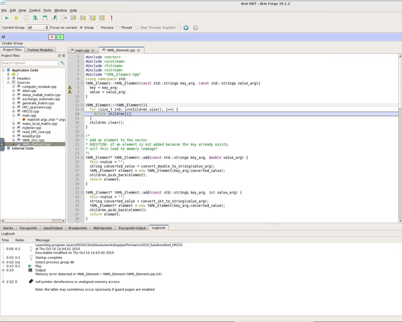
When DDT stops on the segmentation fault, the stack is in the YAML_Element::~YAML_Element function of YAML_Element.cpp. Looking at this function, we see that the loop stops at children.size() instead of children.size()-1. So, line 13 should be changed from
for(size_t i=0; i<=children.size(); i++) {
to
for(size_t i=0; i<children.size(); i++) {
Hardware
On Pitzer, there are 40 cores per node (20 cores per socket and 2 sockets per node). There is support for AVX512, vector length 8 double or 16 single precision values and fused multiply-add. (There is hardware support for 4 thread per core, but it is currently not enabled on OSC systems.)
There are three cache levels on Pitzer, and the statistics are shown in the table below:
| Cache level | Size (KB) | Latency (cycles) | Max BW (bytes/cycle) | Sustained BW (bytes/cycle) |
|---|---|---|---|---|
| L1 DCU | 32 | 4-6 | 192 | 133 |
| L2 MLC | 1024 | 14 | 64 | 52 |
| L3 LLC | 28160 | 50-70 | 16 | 15 |
Never do heavy I/O in your home directory. Home directories are for long-term storage, not scratch files.
One option for I/O intensive jobs is to use the local disk on a compute node. Stage files to and from your home directory into $TMPDIR using the pbsdcp command (e.g. pbsdcp file1 file2 $TMPDIR), and execute the program in $TMPDIR.
Another option is to use the scratch file system ($PFSDIR). This is faster than other file systems, good for parallel jobs, and may be faster than local disk.
For more information about OSC's file system, click here.
For example batch scripts showing the use of $TMPDIR and $PFSDIR, click here.
For more information about Pitzer, click here.
Performance Measurement
FLOPS stands for "floating point operations per second." Pitzer has a theoretical maximum of 720 teraflops. With the LINPACK benchmark of solving a dense system of linear equations, 543 teraflops. With the STREAM benchmark, which measures sustainable memory bandwidth and the corresponding computation rate for vector kernels, copy: 299095.01 MB/s, scale: 298741.01 MB/s, add: 331719.18 MB/s, and traid: 331712.19 MB/s. Application performance is typically much less than peak/sustained performance since applications usually do not take full advantage of all hardware features.
Timing
You can time a program using the /usr/bin/time command. It gives results for user time (CPU time spent running your program), system time (CPU time spent by your program in system calls), and elapsed time (wallclock). It also shows % CPU, which is (user + system) / elapsed, as well as memory, pagefault, swap, and I/O statistics.
/usr/bin/time j3
5415.03user 13.75system 1:30:29elapsed 99%CPU \
(0avgtext+0avgdata 0maxresident)k \
0inputs+0outputs (255major+509333minor)pagefaults 0 swaps
You can also time portions of your code:
| C/C++ | Fortran 77/90 | MPI (C/C++/Fortran) | |
|---|---|---|---|
| Wallclock |
time(2), difftime(3), getrusage(2) |
SYSTEM_CLOCK(2) | MPI_Wtime(3) |
| CPU | times(2) | DTIME(3), ETIME(3) | X |
Profiling
A profiler can show you whether code is compute-bound, memory-bound, or communication bound. Also, it shows how well the code uses available resources and how much time is spent in different parts of your code. OSC has the following profiling tools: ARM Performance Reports, ARM MAP, Intel VTune, Intel Trace Analyzer and Collector (ITAC), Intel Advisor, TAU Commander, and HPCToolkit.
For profiling, use the -g flag and specify the same optimization level that you normally would normally use with -On. For example:
icc -g -O3 -o mycode mycode.c
Look for
- Hot spots (where most of the time is spent)
- Excessive number of calls to short functions (use inlining!)
- Memory usage (swapping and thrashing are not allowed at OSC)
- % CPU (low CPU utilization may mean excessive I/O delays).
ARM Performance Reports
ARM PR works on precompiled binaries, so the -g flag is not needed. It gives a summary of your code's performance that you can view with a browser.
For a non-MPI program:
module load arm-pr
perf-report --no-mpi ./mycode [args]
For an MPI program:
module load arm-pr
perf-report --np num_procs ./mycode [args]
ARM MAP
Interpreting this profile requires some expertise. It gives details about your code's performance. You can view and explore the resulting profile using an ARM client.
For a non-MPI program:
module load arm-map
map --no-mpi ./mycode [args]
For an MPI program:
module load arm-pr
map --np num_procs ./mycode [args]
For more information about ARM Tools, view OSC resources or visit ARM's website.
Intel Trace Analyzer and Collector (ITAC)
ITAC is a graphical tool for profiling MPI code (Intel MPI).
To use:
module load intelmpi # then compile (-g) code
mpiexec -trace ./mycode
View and explore the results using a GUI with traceanalyzer:
traceanalyzer <mycode>.stf
Help From the Compiler
HPC software is traditionally written in Fortran or C/C++. OSC supports several compiler families. Intel (icc, icpc, ifort) usually gives fastest code on Intel architecture). Portland Group (PGI - pgcc, pgc++, pgf90) is good for GPU programming, OpenACC. GNU (gcc, g++, gfortran) is open source and universally available.
Compiler options are easy to use and let you control aspects of the optimization. Keep in mind that different compilers have different values for options. For all compilers, any highly optimized builds, such as those employing the options herein, should be thoroughly validated for correctness.
Some examples of optimization include:
- Function inlining (eliminating function calls)
- Interprocedural optimization/analysis (ipo/ipa)
- Loop transformations (unrolling, interchange, splitting, tiling)
- Vectorization (operate on arrays of operands)
- Automatic parallization of loops (very conservative multithreading)
Compiler flags to try first are:
- General optimization flags (-O2, -O3, -fast)
- Fast math
- Interprocedural optimization/analysis
Faster operations are sometimes less accurate. For Intel compilers, fast math is default with -O2 and -O3. If you have a problem, use -fp-model precise. For GNU compilers, precise math is default with -O2 and -O3. If you want faster performance, use -ffast-math.
Inlining is replacing a subroutine or function call with the actual body of the subprogram. It eliminates overhead of calling the subprogram and allows for more loop optimizations. Inlining for one source file is typically automatic with -O2 and -O3.
Optimization Compiler Options
Options for Intel compilers are shown below. Don't use -fast for MPI programs with Intel compilers. Use the same compiler command to link for -ipo with separate compilation. Many other optimization options can be found in the man pages. The recommended options are -O3 -xHost. An example is ifort -O3 program.f90.
| -fast | Common optimizations |
| -On |
Set optimization level (0, 1, 2, 3) |
| -ipo | Interprocedural optimization, multiple files |
| -O3 | Loop transforms |
| -xHost | Use highest instruction set available |
| -parallel | Loop auto-parallelization |
Options for PGI compilers are shown below. Use the same compiler command to link for -Mipa with separate compilation. Many other optimization options can be found in the man pages. The recommended option is -fast. An example is pgf90 -fast program.f90.
| -fast | Common optimizations |
| -On |
Set optimization level (0, 1, 2, 3, 4) |
| -Mipa | Interprocedural optimization |
| -Mconcur | Loop auto-parallelization |
Options for GNU compilers are shown below. Use the same compiler command to link for -Mipa with separate compilation. Many other optimization options can be found in the man pages. The recommended options are -O3 -ffast-math. An example is gfortran -O3 program.f90.
| -On | Set optimization level (0, 1, 2, 3) |
| N/A for separate compilation | Interprocedural optimization |
| -O3 | Loop transforms |
| -ffast-math | Possibly unsafe floating point optimizations |
| -march=native | Use highest instruction set available |
Hands On
Compile and run with different compiler options:
time srun -n 2 ./test_HPCCG 150 150 150
Using the optimal compiler flags, get an overview of the bottlenecks in the code with the ARM performance report:
module load arm-pr
perf-report -np 2 ./test_HPCCG 150 150 150
Solution
On Pitzer, sample times were:
| Compiler Option | Runtime (seconds) |
|---|---|
| -g | 129 |
| -O0 -g | 129 |
| -O1 -g | 74 |
| -O2 -g | 74 |
| -O3 -g |
74 |
The performance report shows that the code is compute-bound.
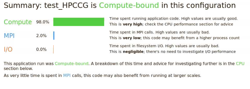
Compiler Optimization Reports
Compiler optimization reports let you understand how well the compiler is doing at optimizing your code and what parts of your code need work. They are generated at compile time and describe what optimizations were applied at various points in the source code. The report may tell you why optimizations could not be performed.
For Intel compilers, -qopt-report and outputs to a file.
For Portland Group compilers, -Minfo and outputs to stderr.
For GNU compilers, -fopt-info and ouputs to stderr by default.
A sample output is:
LOOP BEGIN at laplace-good.f(10,7)
   remark #15542: loop was not vectorized: inner loop was already vectorized

   LOOP BEGIN at laplace-good.f(11,10)
   <Peeled loop for vectorization>
   LOOP END

   LOOP BEGIN at laplace-good.f(11,10)
      remark #15300: LOOP WAS VECTORIZED
   LOOP END

   LOOP BEGIN at laplace-good.f(11,10)
   <Remainder loop for vectorization>
      remark #15301: REMAINDER LOOP WAS VECTORIZED
   LOOP END

   LOOP BEGIN at laplace-good.f(11,10)
   <Remainder loop for vectorization>
   LOOP END
LOOP END
Hands On
Add the compiler flag -qopt-report=5 and recompile to view an optimization report.
Vectorization/Streaming
Code is structured to operate on arrays of operands. Vector instructions are built into the processor. On Pitzer, the vector length is 16 single or 8 double precision. The following is a vectorizable loop:
do i = 1,N
  a(i) = b(i) + x(1) * c(i)
end do
Some things that can inhibit vectorization are:
- Loops being in the wrong order (usually fixed by compiler)
- Loops over derived types
- Function calls (can sometimes be fixed by inlining)
- Too many conditionals
- Indexed array accesses
Hands On
Use ARM MAP to identify the most expensive parts of the code.
module load arm-map
map -np 2 ./test_HPCCG 150 150 150
Check the optimization report previously generated by the compiler (with -qopt-report=5) to see if any of the loops in the regions of the code are not being vectorized. Modify the code to enable vectorization and rerun the code.
Solution
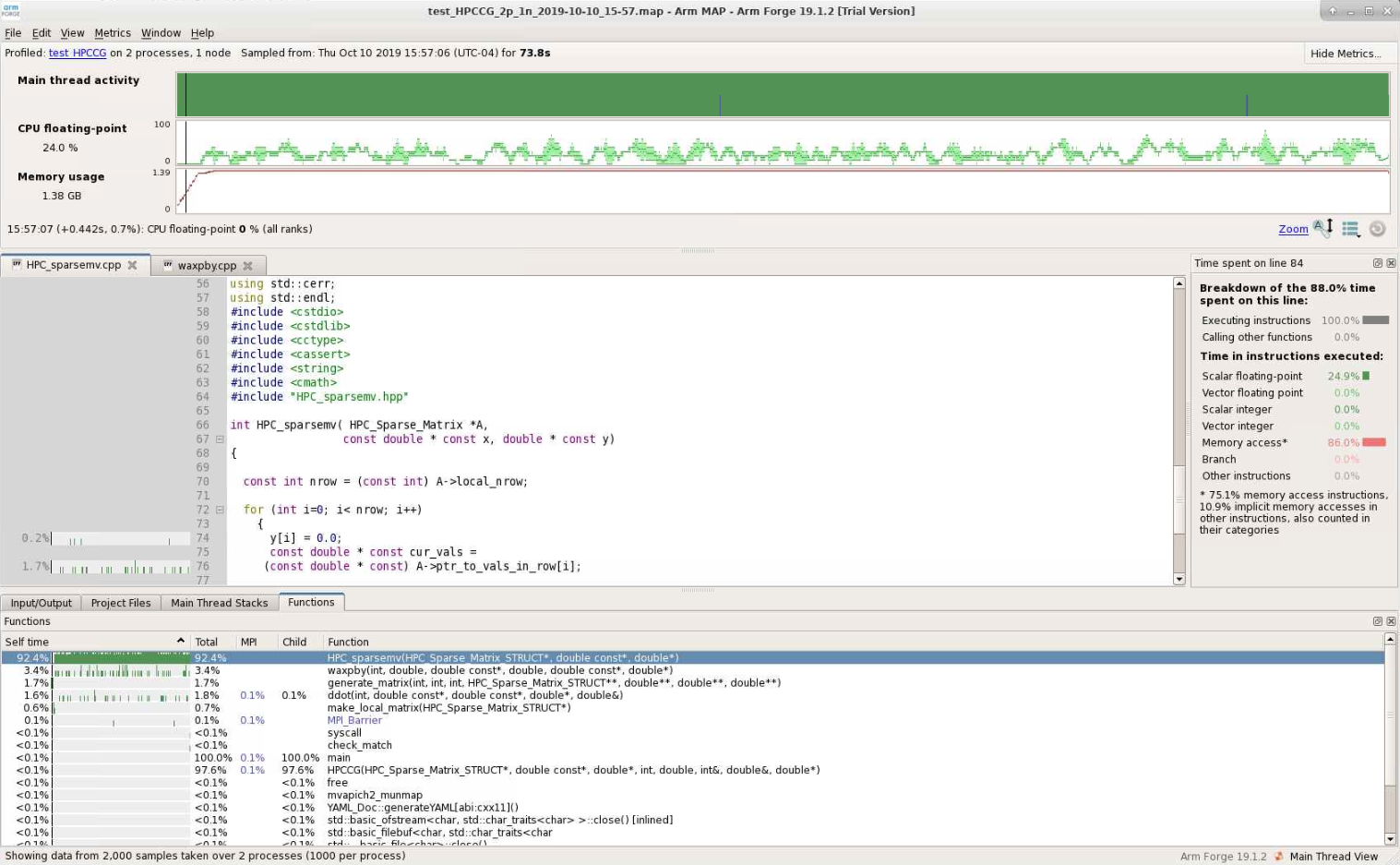 Map shows that the most expensive segment of the code is lines 83-84 of HPC_sparsemv.cpp:
for (int j=0; j< cur_nnz; j++)
  y[i] += cur_vals[j]*x[cur_inds[j]];
The optimization report confirms that the loop was not vectorized due to a dependence on y.
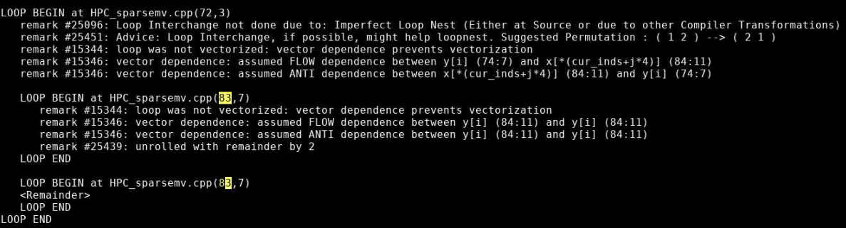
Incrementing a temporary variable instead of y[i], should enable vectorization:
for (int j=0; j< cur_nnz; j++)
  sum += cur_vals[j]*x[cur_inds[j]];
y[i] = sum;
Recompiling and rerunning with change reduces runtime from 74 seconds to 63 seconds.
Memory access is often the most important factor in your code's performance. Loops that work with arrays should use a stride of one whenever possible. C and C++ are row-major (store elements consecutively by row in 2D arrays), so the first array index should be the outermost loop and the last array index should be the innermost loop. Fortran is column-major, so the reverse is true. You can get factor of 3 or 4 speedup just by using unit stride. Avoid using arrays of derived data types, structs, or classes. For example, use structs of arrays instead of arrays of structures.
Efficient cache usage is important. Cache lines are 8 words (64 bytes) of consecutive memory. The entire cache line is loaded when a piece of data is fetched.
The code below is a good example. 2 cache lines are used for every 8 loop iterations, and it is unit stride:
real*8 a(N), b(N)
do i = 1,N
  a(i) = a(i) + b(i)
end do

! 2 cache lines:
! a(1), a(2), a(3) ... a(8)
! b(1), b(2), b(3) ... b(8)
The code below is a bad example. 1 cache line is loaded for each loop iteration, and it is not unit stride:
TYPE :: node
  real*8 a, b, c, d, w, x, y, z
END TYPE node
TYPE(node) :: s(N)
do i = 1, N
  s(i)%a = s(i)%a + s(i)%b
end do

! cache line:
! a(1), b(1), c(1), d(1), w(1), x(1), y(1), z(1)
Hands On
Look again at the most expensive parts of the code using ARM MAP:
module load arm-map
map -np 2 ./test_HPCCG 150 150 150
Look for any inefficient memory access patterns. Modify the code to improve memory access patterns and rerun the code. Do these changes improve performance?
Solution
Lines 110-148 of generate_matrix.cpp are nested loops:
for (int ix=0; ix<nx; ix++) {
  for (int iy=0; iy<ny; iy++) {
    for (int iz=0; iz<nz; iz++) {
      int curlocalrow = iz*nx*ny+iy*nx+ix;
      int currow = start_row+iz*nx*ny+iy*nx+ix;
      int nnzrow = 0;
      (*A)->ptr_to_vals_in_row[curlocalrow] = curvalptr;
      (*A)->ptr_to_inds_in_row[curlocalrow] = curindptr;
      .
      .
      .
    }
  }
}
The arrays are accessed in a manner so that consecutive values of ix are accesssed in order. However, our loops are ordered so that the ix is the outer loop. We can reorder the loops so that ix is iterated in the inner loop:
for (int iz=0; iz<nz; iz++) {
  for (int iy=0; iy<ny; iy++) {
    for (int ix=0; ix<nx; ix++) {
      .
      .
      .
    }
  }
}
This reduces the runtime from 63 seconds to 22 seconds.
OpenMP
OpenMP is a shared-memory, threaded parallel programming model. It is a portable standard with a set of compiler directives and a library of support functions. It is supported in compilers by Intel, Portland Group, GNU, and Cray.
The following are parallel loop execution examples in Fortran and C. The inner loop vectorizes while the outer loop executes on multiple threads:
PROGRAM omploop
INTEGER, PARAMETER :: N = 1000
INTEGER i, j
REAL, DIMENSION(N, N) :: a, b, c, x
... ! Initialize arrays
!$OMP PARALLEL DO
do j = 1, N
  do i = 1, N
    a(i, j) = b(i, j) + x(i, j) * c(i, j)
  end do
end do
!$OMP END PARALLEL DO
END PROGRAM omploop
int main() {
  int N = 1000;
  float *a, *b, *c, *x;
... // Allocate and initialize arrays
#pragma omp parallel for
  for (int i = 0; i < N; i++) {
    for (int j = 0; j < N; j++) {
      a[i*N+j] = b[i*N+j] + x[i*N+j] * c[i*N+j]
    }
  }
}
You can add an option to compile a program with OpenMP.
For Intel compilers, add the -qopenmp option. For example, ifort -qopenmp ompex.f90 -o ompex.
For GNU compilers, add the -fopenmp option. For example, gcc -fopenmp ompex.c -o ompex.
For Portland group compilers, add the -mp option. For example, pgf90 -mp ompex.f90 -o ompex.
To run an OpenMP program, requires multiple processors through Slurm (--N 1 -n 40) and set the OMP_NUM_THREADS environment variable (default is use all available cores). For the best performance, run at most one thread per core.
An example script is:
#!/bin/bash
#SBATCH -J omploop
#SBATCH -N 1
#SBATCH -n 40
#SBATCH -t 1:00

export OMP_NUM_THREADS=40
/usr/bin/time ./omploop
For more information, visit http://www.openmp.org, OpenMP Application Program Interface, and self-paced turorials. OSC will host an XSEDE OpenMP workshop on November 5, 2019.
MPI
MPI stands for message passing interface for when multiple processes run on one or more nodes. MPI has functions for point-to-point communication (e.g. MPI_Send, MPI_Recv). It also provides a number of functions for typical collective communication patterns, including MPI_Bcast (broadcasts value from root process to all other processes), MPI_Reduce (reduces values on all processes to a single value on a root process), MPI_Allreduce (reduces value on all processes to a single value and distributes the result back to all processes), MPI_Gather (gathers together values from a group of processes to a root process), and MPI_Alltoall (sends data from all processes to all processes).
A simple MPI program is:
#include <mpi.h>
#include <stdio.h>

int main(int argc, char *argv[]) {
  int rank, size;
  MPI_INIT(&argc, &argv);
  MPI_Comm_rank(MPI_COMM_WORLD, &rank);
  MPI_COMM_size(MPI_COMM_WORLD, &size);
  printf("Hello from node %d of %d\n", rank size);
  MPI_Finalize();
  return(0);
}
MPI implementations available at OSC are mvapich2, Intel MPI (only for Intel compilers), and OpenMPI.
MPI programs can be compiled with MPI compiler wrappers (mpicc, mpicxx, mpif90). They accept the same arguments as the compilers they wrap. For example, mpicc -o hello hello.c.
MPI programs must run in batch only. Debugging runs may be done with interactive batch jobs. srun automatically determines exectuion nodes from PBS:
#!/bin/bash
#SBATCH -J mpi_hello
#SBATCH -N 2
#SBATCH --ntasks-per-node=40
#SBATCH -t 1:00

cd $PBS_O_WORKDIR
srun ./hello
For more information about MPI, visit MPI Forum and MPI: A Message-Passing Interface Standard. OSC will host an XSEDE MPI workshop on September 3-4, 2019. Self-paced tutorials are available here.
Hands On
Use ITAC to get a timeline of the run of the code.
module load intelmpi
LD_PRELOAD=libVT.so \
mpiexec -trace -np 40 ./test_HPCCG 150 150 150
traceanalyzer <stf_file>
Look at the Event Timeline (under Charts). Do you see any communication patterns that could be replaced by a single MPI command?
Solution
Looking at the Event Timeline, we see that a large part of runtime is spent in the following communication pattern: MPI_Barrier, MPI_Send/MPI_Recv, MPI_Barrier. We also see that during this communication rank 0 is sending data to all other rank. We should be able to replace all of these MPI calls with a single call to MPI_Bcast.
The relavent code is in lines 82-89 of ddot.cpp:
  MPI_Barrier(MPI_COMM_WORLD);
  if(rank == 0) {
    for(int dst_rank=1; dst_rank < size; dst_rank++) {
      MPI_Send(&global_result, 1, MPI_DOUBLE, dst_rank, 1, MPI_COMM_WORLD);
    }
  }
  if(rank != 0) MPI_Recv(&global_result, 1, MPI_DOUBLE, 0, 1, MPI_COMM_WORLD, MPI_STATUS_IGNORE);
  MPI_Barrier(MPI_COMM_WORLD);
and can be replaced with:
MPI_Bcast(&global_result, 1, MPI_DOUBLE, 0, MPI_COMM_WORLD);
Interpreted Languages
Although many of the tools we already mentioned can also be used with interpreted languages, most interpreted languages such as Python and R have their own profiling tools.
Since they are still running on th same hardware, the performance considerations are very similar for interpreted languages as they are for compiled languages:
- Vectorization
- Efficient memory utilization
- Use built-in and library functions where possible
- Use appropriate data structures
- Understand and use best practices for the language
One of Python's most common profiling tools is cProfile. The simplest way to use cProfile is to add several arguments to your Python call so that an ordered list of the time spent in all functions called during executation. For instance, if a program is typically run with the command:
python ./mycode.py
replace that with
python -m cProfile -s time ./mycode.py
Here is a sample output from this profiler: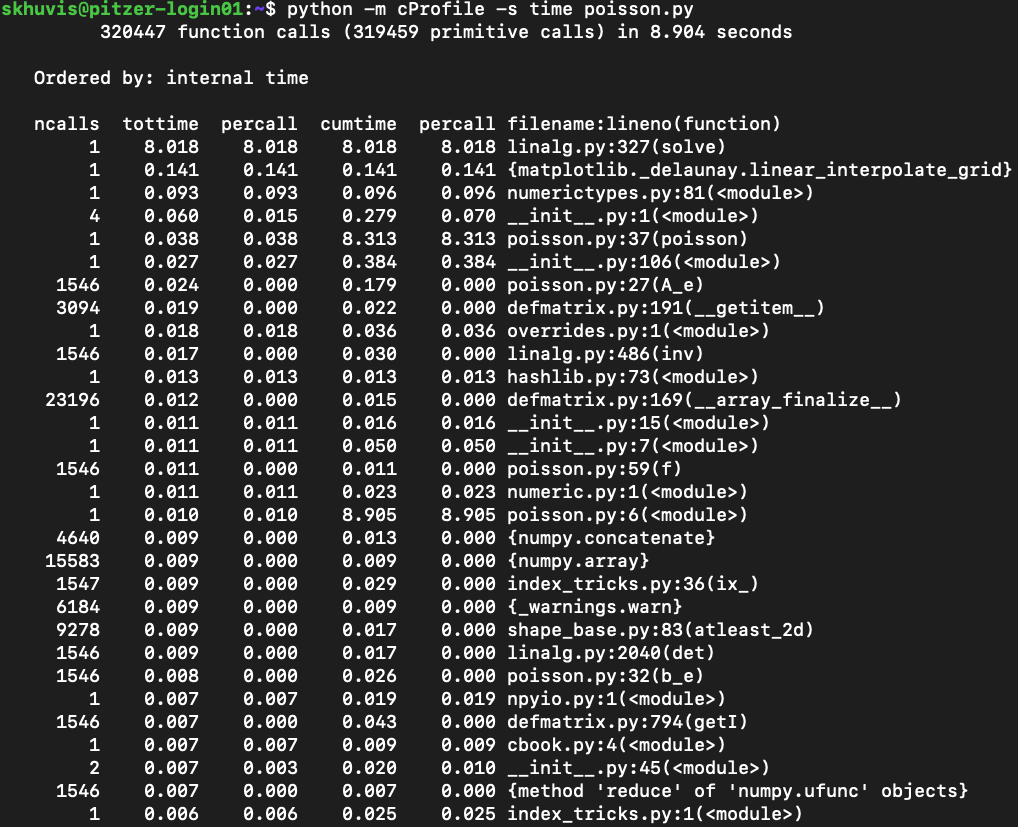
See Python's documentation for more details on how to use cProfile.
One of the most popular profilers for R is profvis. It is not available by default with R so it will need to be installed locally before its first use and loaded into your environment prior to each use. To profile your code, just put how you would usually call your code as the argument into profvis:
$ R
> install.packages('profvis')
> library('profvis')
> profvis({source('mycode.R')}
Here is a sample output from profvis: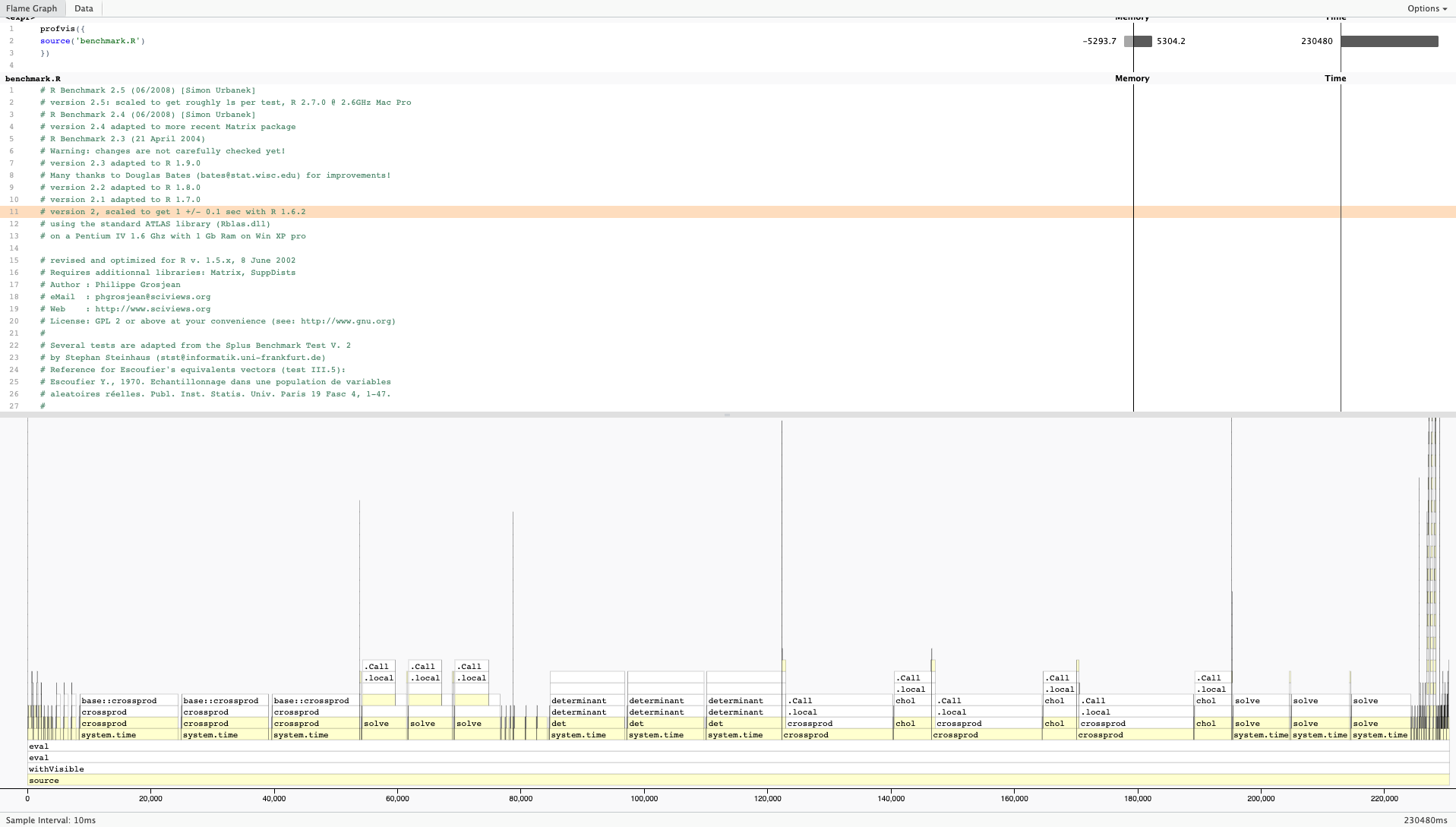
For more information on profvis is available here.
Hands On
Python
First, enter the Python/ subdirectory of the code containing the python script ns.py. Profile this code with cProfile to determine the most expensive functions of the code. Next, rerun and profile with the array as an argument to ns.py. Which versions runs faster? Can you determine why it runs faster?
Solution
Execute the following commands:
python -m cProfile -s time ./ns.py
python -m cProfile -s time ./ns.py array
In the original code, 66 seconds out 68 seconds are spent in presPoissPeriodic. When the array argument is passed, the time spent in this function is approximately 1 second and the total runtime goes down to about 2 seconds.
The speedup comes from the vectorization of the main computation in the body of presPoissPeriodic by replacing nester for loops with a single like operation on arrays.
R
Now, enter the R/ subdirectory of the code containing the R script lu.R. Make sure that you have the R module loaded. First, run the code with profvis without any additional arguments and then again with frmt="matrix".
Which version of the code runs faster? Can you tell why it runs faster based on the profile?
Solution
Runtime for the default version is 28 seconds while the runtime when frmt="matrix" is 20 seconds.
Here is the profile with default arguments: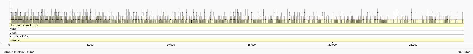
And here is the profile with frmt="matrix":
We can see that most of the time is being spent in lu_decomposition. The difference, however, is that the dataframe version seems to have a much higher overhead associated with accessing elements of the dataframe. On the other hand, the profile of the matrix version seems to be much flatter with fewer functions being called during LU decomposition. This reduction in overhead by using a matrix instead of a dataframe results in the better performance.
Tag:
Service:
Technologies:
HOWTO: Tune VASP Memory Usage
This article discusses memory tuning strategies for VASP.
Data Distribution
Typically the first approach for memory sensitive VASP issues is to tweak the data distribution (via NCORE or NPAR). The information at https://www.vasp.at/wiki/index.php/NPAR covers a variety of machines. OSC has fast communications via Infiniband.
Performance and memory consumption are dependent on the simulation model. So we recommend a series of benchmarks varying the number of nodes and NCORE. The recommended initial value for NCORE is the processor count per node which is the ntasks-per-node value in Slurm (the ppn value in PBS). Of course, if this benchmarking is intractable then one must reexamine the model. For general points see: https://www.vasp.at/wiki/index.php/Memory_requirements and https://www.vasp.at/wiki/index.php/Not_enough_memory And of course one should start small and incrementally improve or scale up one's model.
Rationalization
Using the key parameters with respect to memory scaling listed at the VASP memory requirements page one can rationalize VASP memory usage. The general approach is to study working calculations and then apply that understanding to scaled up or failing calculations. This might help one identify if a calculation is close to a node's memory limit and happens to cross over the limit for reasons that might be out of ones control, in which case one might need to switch to higher memory nodes.
Here is an example of rationalizing memory consumption. Extract from a simulation output the key parameters:
Dimension of arrays:
k-points NKPTS = 18 k-points in BZ NKDIM = 18 number of bands NBANDS= 1344
total plane-waves NPLWV = 752640
...
dimension x,y,z NGXF= 160 NGYF= 168 NGZF= 224
support grid NGXF= 320 NGYF= 336 NGZF= 448
This yields 273 GB of memory, NKDIM*NBANDS*NPLWV*16 + 4*(NGXF/2+1)*NGYF*NGZF*16, according to
https://www.vasp.at/wiki/index.php/Memory_requirements
This estimate should be compared to actual memory reports. See for example XDModD and grafana. Note that most application software has an overhead in the ballpack of ten to twenty percent. In addition, disk caching can consume significant memory. Thus, one must adjust the memory estimate upward. It can then be comapred to the available memory per cluster and per cluster node type.
Miscellaneous
- OSC sets the default resource limits for shells, except for core dump file size, to unlimited; see the limit/ulimit/unlimit commands depending on your shell.
- In the INCAR input file NWRITE=3 is for verbose output and NWRITE=4 is for debugging output.
- OSC does not have a VASP license and our staff has limited experience with it. So investigate alternate forms of help: ask within your research group and post on the VASP mailing list.
- Valgrind is a tool that can be used for many types of debugging including looking for memory corruptions and leaks. However, it slows down your code a very sizeable amount. This might not be feasible for HPC codes
- ASAN (address sanitizer) is another tool that can be used for memory debugging. It is less featureful than Valgrind, but runs much quicker, and so will likely work with your HPC code.
Service:
HOWTO: Use 'rclone' to Upload Data
rclone is a tool that can be used to upload and download files to a cloud storage (like Microsoft OneDrive, BuckeyeBox) from the command line. It's shipped as a standalone binary, but requires some user configuration before using. In this page, we will provide instructions on how to use rclone to upload data to OneDrive. For instructions with other cloud storage, check rclone Online documentation.
You can use "Globus" feature of OnDemand to perform data transfer between OneDrive and other storage. See this File Transfer and Management page for more information.
Setup
Before configuration, please first log into OSC OnDemand and request a Pitzer Lightweight Desktop session. Walltime of 1 hour should be sufficient to finish the configuration.
Note: this does not work with the 'konqueror' browser present on OSC Systems. Please set default to Firefox first before you do the setup following the instructions below:
* xfce: Applications (Top left corner) -> Settings -> Preferred Applications
* mate: System (top bar towards the left) -> Preferences -> Preferred Applications
* xfce: Applications (Top left corner) -> Settings -> Preferred Applications
* mate: System (top bar towards the left) -> Preferences -> Preferred Applications
Once the session is ready, open a terminal. In the terminal, run the command
rclone config
It prompts you with a bunch of questions:
- It shows "No remotes found -- make a new one" or list available remotes you made before
- Answer "n" for "New remote"
- "name>" (the name for the new remote)
- Type "OneDrive" (or whatever else you want to call this remote)
- "Storage>" (the storage type of the new remote)
- This should display a list to choose from. Enter the number corresponding to the "Microsoft OneDrive" storage type, which is "26".
- (It is "6" for BuckeyeBox)
- "client_id>"
- Leave this blank (just press enter).
- "client_secret>"
- Leave this blank (just press enter).
- "Edit advanced config?"
- Type "n" for no
- "Use auto config?"
- Answer "y" for yes
- A web browser window should pop up allowing you to log into box. It is a good idea at this point to verify that the url is actually OneDrive before entering any credentials
- Enter your OSU email
- This should take you to the OSU login page. Login with your OSU credentials
- Go back to the terminal once "Success" is displayed.
- "Your choice>"
- One of five options to locate the drive you wish to use.
- Type "1" to use your personal or business OneDrive
- "Choose drive to use"
- Type "0"
- "Is this Okay? y/n>"
- Type "y" to confirm the drive you wish to use is correct.
- "y/e/d>"
- Type "y" to confirm you wish to add this remote to rclone.
Testing rclone
Note: you do not need to use Pitzer Lightweight Desktop when you run 'rclone'. You can test the data transfer with a small file using login nodes (either Pitzer or Owens), or request a regular compute node to do the data transfer with large files.
Create an empty hello.txt file and upload it to OneDrive using 'rclone copy' as below in a terminal:
touch hello.txt
rclone copy hello.txt OneDrive:/test
This creates a toplevel directory in OneDrive called 'test' if it does not already exist, and uploads the file hello.txt to it.
To verify the uploading is successful, you can either login to OneDrive in a web browser to check the file, or use rclone ls command in the terminal as:
rclone ls OneDrive:/test
Note: be careful when using
ls on a large directory, because it's recursive. You can add a '--max-depth 1' flag to stop the recursion. Downloading from OneDrive to OSC
Copy the contents of a source directory from a configured OneDrive remote, OneDrive:/src/dir/path, into a destination directory in your OSC session, /dest/dir/path, using the code below:
rclone copy OneDrive:/src/dir/path /dest/dir/path
Identical files on the source and destination directories are not transferred. Only the contents of the provided source directory are copied, not the directory name and contents.
copy does not delete files from the destination. To delete files from the destination directory in order to match the source directory, use the sync command instead.
If only one file is being transferred, use the copyto command instead.
Note: The
--no-traverse option can be used to increase efficiency by stopping rclone from listing the destination. It should be used when copying a small number of files and/or have a large number of files on the destination, but not when a large number of files are being copied.Note: Shared folders will not appear when listing a directory they are filed in. They are still accessible and data can be move to/from them. For example, the commands
rclone ls OneDrive:/path/to/shared_folder and rclone copy OneDrive:/path/to/shared_folder /dest/dir/path will work normally even though the shared folder does not appear when listing their source directory.Limitations
If rclone remains unused for 90 days, the refresh token will expire, leading to issues with authorization. This can be easily resolved by executing the rclone config reconnect remote: command, which generates a fresh token and refresh token.
Naming
It's important to note OneDrive is case insensitive which prohibits the coexistence files such as "Hello.doc" and "hello.doc". Certain characters are prohibited from being in OneDrive filenames and are commonly encountered on non-Windows platforms. Rclone addresses this by converting these filenames to their visually equivalent Unicode alternatives.
File Sizes
The largest allowed file size is 250 GiB for both OneDrive Personal and OneDrive for Business (Updated 13 Jan 2021).
Path Length
The entire path, including the file name, must contain fewer than 400 characters for OneDrive, OneDrive for Business and SharePoint Online. It is important to know the limitation when encrypting file and folder names with rclone, as the encrypted names are typically longer than the original ones.
Number of Files
OneDrive seems to be OK with at least 50,000 files in a folder, but at 100,000 rclone will get errors listing the directory like couldn’t list files: UnknownError:.
Reference
HOWTO: Use 'rclone' to Upload Data from Google Drive
rclone is a tool that can be used to upload and download files to a cloud storage (like Microsoft OneDrive, BuckeyeBox) from the command line. It's shipped as a standalone binary, but requires some user configuration before using. In this page, we will provide instructions on how to use rclone to upload data from Google Drive. For instructions with other cloud storage, check rclone Online documentation.
Setup
Before configuration, please first log into OSC OnDemand and request a Pitzer Lightweight Desktop session. Walltime of 1 hour should be sufficient to finish the configuration.
Once the session is ready, open a terminal. In the terminal, run the command
rclone config
It prompts you with a bunch of questions:
- It shows "No remotes found -- make a new one" or list available remotes you made before
- Answer "n" for "New remote"
- "name>" (the name for the new remote)
- Type "GDrive" (or whatever else you want to call this remote)
- "Storage>" (the storage type of the new remote)
- This should display a list to choose from. Enter the number corresponding to the "Google Drive" storage type, which is "15".
- "client_id>"
- Leave this blank (just press enter).
- "client_secret>"
- Leave this blank (just press enter).
- Scope that rclone should use when requesting access from drive.
Enter a string value. Press Enter for the default ("").
Choose a number from below, or type in your own value- Select "2" for read-only access.
- "Edit advanced config?"
- Type "n" for no
- "Use auto config?"
- Answer "y" for yes
- A web browser window should pop up allowing you to log into Google. It is a good idea at this point to verify that the URL is actually Google before entering any credentials. You may also copy and paste the link from Terminal into a web browser.
- Enter your Google credentials
Downloading from Google Drive to OSC
Copy the contents of a source directory from a configured OneDrive remote, GDrive:/src/dir/path, into a destination directory in your OSC session, /dest/dir/path, using the code below:
rclone copy GDrive:/src/dir/path /dest/dir/path --progress
Identical files on the source and destination directories are not transferred. Only the contents of the provided source directory are copied, not the directory name and contents.
copy does not delete files from the destination. To delete files from the destination directory in order to match the source directory, use the sync command instead.
If only one file is being transferred, use the copyto command instead.
Note: The
--no-traverse option can be used to increase efficiency by stopping rclone from listing the destination. It should be used when copying a small number of files and/or have a large number of files on the destination, but not when a large number of files are being copied.Note: Shared folders will not appear when listing a directory they are filed in. They are still accessible and data can be move to/from them. For example, the commands
rclone ls GDrive:/path/to/shared_folder and rclone copy GDrive:/path/to/shared_folder /dest/dir/path will work normally even though the shared folder does not appear when listing their source directory.Limitations
If rclone remains unused for 90 days, the refresh token will expire, leading to issues with authorization. This can be easily resolved by executing the rclone config reconnect remote: command, which generates a fresh token and refresh token.
Naming
It's important to note Google Drive is case insensitive which prohibits the coexistence files such as "Hello.doc" and "hello.doc". Certain characters are prohibited from being in Google Drive filenames and are commonly encountered on non-Windows platforms. Rclone addresses this by converting these filenames to their visually equivalent Unicode alternatives.
Reference
HOWTO: Use Address Sanitizer
Address Sanitizer is a tool developed by Google detect memory access error such as use-after-free and memory leaks. It is built into GCC versions >= 4.8 and can be used on both C and C++ codes. Address Sanitizer uses runtime instrumentation to track memory allocations, which mean you must build your code with Address Sanitizer to take advantage of it's features.
There is extensive documentation on the AddressSanitizer Github Wiki.
Memory leaks can increase the total memory used by your program. It's important to properly free memory when it's no longer required. For small programs, loosing a few bytes here and there may not seem like a big deal. However, for long running programs that use gigabytes of memory, avoiding memory leaks becomes increasingly vital. If your program fails to free the memory it uses when it no longer needs it, it can run out of memory, resulting in early termination of the application. AddressSanitizer can help detect these memory leaks.
Additionally, AddressSanitizer can detect use-after-free bugs. A use-after-free bug occurs when a program tries to read or write to memory that has already been freed. This is undefined behavior and can lead to corrupted data, incorrect results, and even program crashes.
Building With Address Sanitzer
We need to use gcc to build our code, so we'll load the gcc module:
module load gnu/9.1.0
The "-fsanitize=address" flag is used to tell the compiler to add AddressSanitizer.
Additionally, due to some environmental configuration settings on OSC systems, we must also statically link against Asan. This is done using the "-static-libasan" flag.
It's helpful to compile the code with debug symbols. AddressSanitizer will print line numbers if debug symbols are present. To do this, add the "-g" flag. Additionally, the "-fno-omit-frame-pointer" flag may be helpful if you find that your stack traces do not look quite correct.
In one command, this looks like:
gcc main.c -o main -fsanitize=address -static-libasan -g
Or, splitting into separate compiling and linking stages:
gcc -c main.c -fsanitize=address -g
gcc main.o -o main -fsanitize=address -static-libasan
Notice that both the compilation and linking steps require the "-fsanitize-address" flag, but only the linking step requires "-static-libasan". If your build system is more complex, it might make sense to put these flags in CFLAGS and LDFLAGS environment variables.
And that's it!
Examples
No Leak
First, let's look at a program that has no memory leaks (noleak.c):
#include <stdio.h>
#include <stdlib.h>
#include <string.h>

int main(int argc, const char *argv[]) {
    char *s = malloc(100);
    strcpy(s, "Hello world!");
    printf("string is: %s\n", s);
    free(s);
    return 0;
}
To build this we run:
gcc noleak.c -o noleak -fsanitize=address -static-libasan -g
And, the output we get after running it:
string is: Hello world!
That looks correct! Since there are no memory leaks in this program, AddressSanitizer did not print anything. But, what happens if there are leaks?
Missing free
Let's look at the above program again, but this time, remove the free call (leak.c):
#include <stdio.h>
#include <stdlib.h>
#include <string.h>

int main(int argc, const char *argv[]) {
    char *s = malloc(100);
    strcpy(s, "Hello world!");
    printf("string is: %s\n", s);
    return 0;
}
Then, to build:
gcc leak.c -o leak -fsanitize=address -static-libasan
And the output:
string is: Hello world!

=================================================================
==235624==ERROR: LeakSanitizer: detected memory leaks

Direct leak of 100 byte(s) in 1 object(s) allocated from:
    #0 0x4eaaa8 in __interceptor_malloc ../../.././libsanitizer/asan/asan_malloc_linux.cc:144
    #1 0x5283dd in main /users/PZS0710/edanish/test/asan/leak.c:6
    #2 0x2b0c29909544 in __libc_start_main (/lib64/libc.so.6+0x22544)

SUMMARY: AddressSanitizer: 100 byte(s) leaked in 1 allocation(s).
This is a leak report from AddressSanitizer. It detected that 100 bytes were allocated, but never freed. Looking at the stack trace that it provides, we can see that the memory was allocated on line 6 in leak.c
Use After Free
Say we found the above leak in our code, and we wanted to fix it. We need to add a call to free. But, what if we add it in the wrong spot?
#include <stdio.h>
#include <stdlib.h>
#include <string.h>

int main(int argc, const char *argv[]) {
    char *s = malloc(100);
    free(s);
    strcpy(s, "Hello world!");
    printf("string is: %s\n", s);
    return 0;
}
The above (uaf.c) is clearly wrong. Albiet a contrived example, the allocated memory, pointed to by "s", was written to and read from after it was freed.
To Build:
gcc uaf.c -o uaf -fsanitize=address -static-libasan
Building it and running it, we get the following report from AddressSanitizer:
=================================================================
==244157==ERROR: AddressSanitizer: heap-use-after-free on address 0x60b0000000f0 at pc 0x00000047a560 bp 0x7ffcdf0d59f0 sp 0x7ffcdf0d51a0
WRITE of size 13 at 0x60b0000000f0 thread T0
    #0 0x47a55f in __interceptor_memcpy ../../.././libsanitizer/sanitizer_common/sanitizer_common_interceptors.inc:790
    #1 0x528403 in main /users/PZS0710/edanish/test/asan/uaf.c:8
    #2 0x2b47dd204544 in __libc_start_main (/lib64/libc.so.6+0x22544)
    #3 0x405f5c  (/users/PZS0710/edanish/test/asan/uaf+0x405f5c)

0x60b0000000f0 is located 0 bytes inside of 100-byte region [0x60b0000000f0,0x60b000000154)
freed by thread T0 here:
    #0 0x4ea6f7 in __interceptor_free ../../.././libsanitizer/asan/asan_malloc_linux.cc:122
    #1 0x5283ed in main /users/PZS0710/edanish/test/asan/uaf.c:7
    #2 0x2b47dd204544 in __libc_start_main (/lib64/libc.so.6+0x22544)

previously allocated by thread T0 here:
    #0 0x4eaaa8 in __interceptor_malloc ../../.././libsanitizer/asan/asan_malloc_linux.cc:144
    #1 0x5283dd in main /users/PZS0710/edanish/test/asan/uaf.c:6
    #2 0x2b47dd204544 in __libc_start_main (/lib64/libc.so.6+0x22544)

SUMMARY: AddressSanitizer: heap-use-after-free ../../.././libsanitizer/sanitizer_common/sanitizer_common_interceptors.inc:790 in __interceptor_memcpy
Shadow bytes around the buggy address:
  0x0c167fff7fc0: 00 00 00 00 00 00 00 00 00 00 00 00 00 00 00 00
  0x0c167fff7fd0: 00 00 00 00 00 00 00 00 00 00 00 00 00 00 00 00
  0x0c167fff7fe0: 00 00 00 00 00 00 00 00 00 00 00 00 00 00 00 00
  0x0c167fff7ff0: 00 00 00 00 00 00 00 00 00 00 00 00 00 00 00 00
  0x0c167fff8000: fa fa fa fa fa fa fa fa fd fd fd fd fd fd fd fd
=>0x0c167fff8010: fd fd fd fd fd fa fa fa fa fa fa fa fa fa[fd]fd
  0x0c167fff8020: fd fd fd fd fd fd fd fd fd fd fd fa fa fa fa fa
  0x0c167fff8030: fa fa fa fa fa fa fa fa fa fa fa fa fa fa fa fa
  0x0c167fff8040: fa fa fa fa fa fa fa fa fa fa fa fa fa fa fa fa
  0x0c167fff8050: fa fa fa fa fa fa fa fa fa fa fa fa fa fa fa fa
  0x0c167fff8060: fa fa fa fa fa fa fa fa fa fa fa fa fa fa fa fa
Shadow byte legend (one shadow byte represents 8 application bytes):
  Addressable:           00
  Partially addressable: 01 02 03 04 05 06 07
  Heap left redzone:       fa
  Freed heap region:       fd
  Stack left redzone:      f1
  Stack mid redzone:       f2
  Stack right redzone:     f3
  Stack after return:      f5
  Stack use after scope:   f8
  Global redzone:          f9
  Global init order:       f6
  Poisoned by user:        f7
  Container overflow:      fc
  Array cookie:            ac
  Intra object redzone:    bb
  ASan internal:           fe
  Left alloca redzone:     ca
  Right alloca redzone:    cb
  Shadow gap:              cc
==244157==ABORTING
This is a bit intimidating. It looks like there's alot going on here, but it's not as bad as it looks. Starting at the top, we see what AddressSanitizer detected. In this case, a "WRITE" of 13 bytes (from our strcpy). Immediately below that, we get a stack trace of where the write occured. This tells us that the write occured on line 8 in uaf.c in the function called "main".
Next, AddressSanitizer reports where the memory was located. We can ignore this for now, but depending on your use case, it could be helpful information.
Two key pieces of information follow. AddressSanitizer tells us where the memory was freed (the "freed by thread T0 here" section), giving us another stack trace indicating the memory was freed on line 7. Then, it reports where it was originally allocated ("previously allocated by thread T0 here:"), line 6 in uaf.c.
This is likely enough information to start to debug the issue. The rest of the report provides details about how the memory is laid out, and exactly which addresses were accessed/written to. You probably won't need to pay too much attention to this section. It's a bit "down in the weeds" for most use cases.
Heap Overflow
AddresssSanitizer can also detect heap overflows. Consider the following code (overflow.c):
#include <stdio.h>
#include <stdlib.h>
#include <string.h>
int main(int argc, const char *argv[]) {
    // whoops, forgot c strings are null-terminated
    // and not enough memory was allocated for the copy
    char *s = malloc(12);
    strcpy(s, "Hello world!");
    printf("string is: %s\n", s);
    free(s);
    return 0;
}
The "Hello world!" string is 13 characters long including the null terminator, but we've only allocated 12 bytes, so the strcpy above will overflow the buffer that was allocated. To build this:
gcc overflow.c -o overflow -fsanitize=address -static-libasan -g -Wall
Then, running it, we get the following report from AddressSanitizer:
==168232==ERROR: AddressSanitizer: heap-buffer-overflow on address 0x60200000003c at pc 0x000000423454 bp 0x7ffdd58700e0 sp 0x7ffdd586f890
WRITE of size 13 at 0x60200000003c thread T0
    #0 0x423453 in __interceptor_memcpy /apps_src/gnu/8.4.0/src/libsanitizer/sanitizer_common/sanitizer_common_interceptors.inc:737
    #1 0x5097c9 in main /users/PZS0710/edanish/test/asan/overflow.c:8
    #2 0x2ad93cbd7544 in __libc_start_main (/lib64/libc.so.6+0x22544)
    #3 0x405d7b  (/users/PZS0710/edanish/test/asan/overflow+0x405d7b)

0x60200000003c is located 0 bytes to the right of 12-byte region [0x602000000030,0x60200000003c)
allocated by thread T0 here:
    #0 0x4cd5d0 in __interceptor_malloc /apps_src/gnu/8.4.0/src/libsanitizer/asan/asan_malloc_linux.cc:86
    #1 0x5097af in main /users/PZS0710/edanish/test/asan/overflow.c:7
    #2 0x2ad93cbd7544 in __libc_start_main (/lib64/libc.so.6+0x22544)

SUMMARY: AddressSanitizer: heap-buffer-overflow /apps_src/gnu/8.4.0/src/libsanitizer/sanitizer_common/sanitizer_common_interceptors.inc:737 in __interceptor_memcpy
Shadow bytes around the buggy address:
  0x0c047fff7fb0: 00 00 00 00 00 00 00 00 00 00 00 00 00 00 00 00
  0x0c047fff7fc0: 00 00 00 00 00 00 00 00 00 00 00 00 00 00 00 00
  0x0c047fff7fd0: 00 00 00 00 00 00 00 00 00 00 00 00 00 00 00 00
  0x0c047fff7fe0: 00 00 00 00 00 00 00 00 00 00 00 00 00 00 00 00
  0x0c047fff7ff0: 00 00 00 00 00 00 00 00 00 00 00 00 00 00 00 00
=>0x0c047fff8000: fa fa 00 fa fa fa 00[04]fa fa fa fa fa fa fa fa
  0x0c047fff8010: fa fa fa fa fa fa fa fa fa fa fa fa fa fa fa fa
  0x0c047fff8020: fa fa fa fa fa fa fa fa fa fa fa fa fa fa fa fa
  0x0c047fff8030: fa fa fa fa fa fa fa fa fa fa fa fa fa fa fa fa
  0x0c047fff8040: fa fa fa fa fa fa fa fa fa fa fa fa fa fa fa fa
  0x0c047fff8050: fa fa fa fa fa fa fa fa fa fa fa fa fa fa fa fa
Shadow byte legend (one shadow byte represents 8 application bytes):
  Addressable:           00
  Partially addressable: 01 02 03 04 05 06 07
  Heap left redzone:       fa
  Freed heap region:       fd
  Stack left redzone:      f1
  Stack mid redzone:       f2
  Stack right redzone:     f3
  Stack after return:      f5
  Stack use after scope:   f8
  Global redzone:          f9
  Global init order:       f6
  Poisoned by user:        f7
  Container overflow:      fc
  Array cookie:            ac
  Intra object redzone:    bb
  ASan internal:           fe
  Left alloca redzone:     ca
  Right alloca redzone:    cb
==168232==ABORTING
This is similar to the use-after-free report we looked at above. It tells us that a heap buffer overflow occured, then goes on to report where the write happened and where the memory was originally allocated. Again, the rest of this report describes the layout of the heap, and probably isn't too important for your use case.
C++ Delete Mismatch
AddressSanitizer can be used on C++ codes as well. Consider the following (bad_delete.cxx):
#include <iostream>
#include <cstring>

int main(int argc, const char *argv[]) {
    char *cstr = new char[100];
    strcpy(cstr, "Hello World");
    std::cout << cstr << std::endl;

    delete cstr;
    return 0;
}
What's the problem here? The memory pointed to by "cstr" was allocated with new[]. An array allocation must be deleted with the delete[] operator, not "delete".
To build this code, just use g++ instead of gcc:
g++ bad_delete.cxx -o bad_delete -fsanitize=address -static-libasan -g
And running it, we get the following output:
Hello World
=================================================================
==257438==ERROR: AddressSanitizer: alloc-dealloc-mismatch (operator new [] vs operator delete) on 0x60b000000040
    #0 0x4d0a78 in operator delete(void*, unsigned long) /apps_src/gnu/8.4.0/src/libsanitizer/asan/asan_new_delete.cc:151
    #1 0x509ea8 in main /users/PZS0710/edanish/test/asan/bad_delete.cxx:9
    #2 0x2b8232878544 in __libc_start_main (/lib64/libc.so.6+0x22544)
    #3 0x40642b  (/users/PZS0710/edanish/test/asan/bad_delete+0x40642b)

0x60b000000040 is located 0 bytes inside of 100-byte region [0x60b000000040,0x60b0000000a4)
allocated by thread T0 here:
    #0 0x4cf840 in operator new[](unsigned long) /apps_src/gnu/8.4.0/src/libsanitizer/asan/asan_new_delete.cc:93
    #1 0x509e5f in main /users/PZS0710/edanish/test/asan/bad_delete.cxx:5
    #2 0x2b8232878544 in __libc_start_main (/lib64/libc.so.6+0x22544)

SUMMARY: AddressSanitizer: alloc-dealloc-mismatch /apps_src/gnu/8.4.0/src/libsanitizer/asan/asan_new_delete.cc:151 in operator delete(void*, unsigned long)
==257438==HINT: if you don't care about these errors you may set ASAN_OPTIONS=alloc_dealloc_mismatch=0
==257438==ABORTING
This is similar to the other AddressSanitizer outputs we've looked at. This time, it tells us there's a mismatch between new and delete. It prints a stack trace for where the delete occured (line 9) and also a stack trace for where to allocation occured (line 5).
Performance
The documentation states:
This tool is very fast. The average slowdown of the instrumented program is ~2x
AddressSanitizer is much faster than tools that do similar analysis such as valgrind. This allows for usage on HPC codes.
However, if you find that AddressSanitizer is too slow for your code, there are compiler flags that can be used to disable it for specific functions. This way, you can use address sanitizer on cooler parts of your code, while manually auditing the hot paths.
The compiler directive to skip analyzing functions is:
__attribute__((no_sanitize_address)
Technologies:
HOWTO: Use Cron and OSCusage for Regular Emailed Reports
It is possible to utilize Cron and the OSCusage command to send regular usage reports via email
Cron
It is easy to create Cron jobs on the Owens and Pitzer clusters at OSC. Cron is a Linux utility which allows the user to schedule a command or script to run automatically at a specific date and time. A cron job is the task that is scheduled.
Shell scripts run as a cron job are usually used to update and modify files or databases; however, they can perform other tasks, for example a cron job can send an email notification.
Getting Help
In order to use what cron has to offer, here is a list of the command name and options that can be used
Usage: crontab [options] file crontab [options] crontab -n [hostname] Options: -udefine user -e edit user's crontab -l list user's crontab -r delete user's crontab -i prompt before deleting -n set host in cluster to run users' crontabs -c get host in cluster to run users' crontabs -s selinux context -x enable debugging
Running a Cron Job
crontab -l
crontab -e
Linux Crontab Format
MIN HOUR DOM MON DOW CMD

Getting Notified by Email Using a Cron Job
* * * * * {cmd} | mail -s "title of the email notification" {your email}
12 15 * * * /opt/osc/bin/OSCusage | mail -s "OSC usage on $(date)" {your email} 2> /path/to/file/for/stdout/and/stderr 2>&1
Using OSCusage
$ /opt/osc/bin/OSCusage --help
usage: OSCusage.py [-h] [-u USER]
[-s {opt,pitzer,glenn,bale,oak,oakley,owens,ruby}] [-A]
[-P PROJECT] [-q] [-H] [-r] [-n] [-v]
[start_date] [end_date]

positional arguments:
start_date start date (default: 2020-04-23)
end_date end date (default: 2020-04-24)

optional arguments:
-h, --help show this help message and exit
-u USER, --user USER username to run as. Be sure to include -P or -A. (default: kalattar)
-s {opt,pitzer,glenn,bale,oak,oakley,owens,ruby}, --system {opt,pitzer,glenn,bale,oak,oakle
-A Show all
-P PROJECT, --project PROJECT project to query (default: PZS0715)
-q show user data
-H show hours
-r show raw
-n show job ID
-v do not summarize
OSCusage 2018-01-24
OSCusage 2018-01-24 2018-01-25
Terminating a Cron Job
ps aux | grep crontab
kill {PID}
crontab -e
HOWTO: Use Docker and Apptainer/Singularity Containers at OSC
It is now possible to run Docker and Apptainer/Singularity containers on the Owens and Pitzer clusters at OSC. Single-node jobs are currently supported, including GPU jobs; MPI jobs are planned for the future.
From the Docker website: "A container image is a lightweight, stand-alone, executable package of a piece of software that includes everything needed to run it: code, runtime, system tools, system libraries, settings."
As of June 21st, 2022, Singularity is replaced with Apptainer, which is just a renamed open-source project. For more information visit the Apptainer/Singularity page
This document will describe how to run Docker and Apptainer/Singularity containers on the Owens and Pitzer. You can use containers from Docker Hub, Sylabs Cloud, or any other source. As examples we will use hello-world from Singularity Hub and ubuntu from Docker Hub.
If you encounter any error, check out Known Issues on using Apptainer/Singularity at OSC. If the issue can not be resolved, please contact OSC help.
Contents
- Getting help
- Setting up your environment
- Access a container
- Run a container
- File system access
- GPU usage within a container
- Build a container
- References
Getting help
The most up-to-date help on Apptainer/Singularity comes from the command itself.
apptainer help
User guides and examples can be found in Apptainer documents.
Setting up your environment for Apptainer/Singularity usage
No setup is required. You can use Apptainer/Singularity directly on all clusters.
Accessing a container
An Apptainer/Singularity container is a single file with a .sif extension.
You can simply download ("pull") a container from a hub. Popular hubs are Docker Hub and Singularity Hub. You can go there and search if they have a container that meets your needs. Docker Hub has more containers and may be more up to date but supports a much wider community than just HPC. Singularity Hub is for HPC, but the number of available containers are fewer. Additionally there are domain and vendor repositories such as biocontainers and NVIDIA HPC containers that may have relevant containers.
Pull a container from hubs
Docker Hub
Pull from the 7.2.0 branch of the gcc repository on Docker Hub. The 7.2.0 is called a tag.
apptainer pull docker://gcc:7.2.0
Filename: gcc_7.2.0.sif
Pull an Ubuntu container from Docker Hub.
apptainer pull docker://ubuntu:18.04
Filename: ubuntu_18.04.sif
Singularity Hub
Pull the singularityhub/hello-world container from the Singularity hub. Since no tag is specified it pulls from the master branch of the repository.
apptainer pull shub://singularityhub/hello-world
Filename: hello-world_latest.sif
Downloading containers from the hubs is not the only way to get one. You can, for example get a copy from your colleague's computer or directory. If you would like to create your own container you can start from the user guide below. If you have any questions, please contact OSC Help.
Running a container
There are four ways to run a container under Apptainer/Singularity.
You can do this either in a batch job or on a login node.
Don’t run on a login node if the container will be performing heavy computation, of course.
If unsure about the amount of memory that a singularity process will require, then be sure to request an entire node for the job. It is common for singularity jobs to be killed by the OOM killer because of using too much RAM.
If unsure about the amount of memory that a singularity process will require, then be sure to request an entire node for the job. It is common for singularity jobs to be killed by the OOM killer because of using too much RAM.
We note that the operating system on Owens is Red Hat:
[owens-login01]$ cat /etc/os-release
NAME="Red Hat Enterprise Linux Server"
VERSION="7.5 (Maipo)"
ID="rhel"
[..more..]
In the examples below we will often check the operating system to show that we are really inside a container.
Run container like a native command
If you simply run the container image it will execute the container’s runscript.
Example: Run singularityhub/hello-world
Note that this container returns you to your native OS after you run it.
[owens-login01]$ ./hello-world_latest.sif
Tacotacotaco
Use the “run” sub-command
The Apptainer “run” sub-command does the same thing as running a container directly as described above. That is, it executes the container’s runscript.
Example: Run a container from a local file
[owens-login01]$ apptainer run hello-world_latest.sif
Tacotacotaco
Example: Run a container from a hub without explicitly downloading it
[owens-login01]$ apptainer run shub://singularityhub/hello-world
INFO: Downloading shub image
Progress |===================================| 100.0%
Tacotacotaco
Use the “exec” sub-command
The Apptainer “exec” sub-command lets you execute an arbitrary command within your container instead of just the runscript.
Example: Find out what operating system the singularityhub/hello-world container uses
[owens-login01]$ apptainer exec hello-world_latest.sif cat /etc/os-release
NAME="Ubuntu"
VERSION="14.04.5 LTS, Trusty Tahr"
ID=ubuntu
[..more..]
Use the “shell” sub-command
The Apptainer “shell” sub-command invokes an interactive shell within a container.
Example: Run an Ubuntu shell. Note the “Apptainer” prompt within the shell.
[owens-login01 ~]$ apptainer shell ubuntu_18.04.sif
Singularity ubuntu_18.04.sif:~> cat /etc/os-release
NAME="Ubuntu"
VERSION="18.04 LTS (Bionic Beaver)"
ID=ubuntu
[.. more ..]
Singularity ubuntu_18.04.sif:~> exit
exit
File system access
When you use a container you run within the container’s environment. The directories available to you by default from the host environment are
- your home directory
- working directory (directory you were in when you ran the container)
/fs/ess/tmp
You can review our Available File Systems page for more details about our file system access policy.
If you run the container within a job you will have the usual access to the $PFSDIR environment variable with adding node attribute "pfsdir" in the job request (--gres=pfsdir). You can access most of our file systems from a container without any special treatment.
GPU usage within a container
If you have a GPU-enabled container you can easily run it on Owens or Pitzer just by adding the --nv flag to the apptainer exec or run command. The example below comes from the "exec" command section of Apptainer User Guide. It runs a TensorFlow example using a GPU on Owens. (Output has been omitted from the example for brevity.)
[owens-login01]$ sinteractive -n 28 -g 1...[o0756]$git clone https://github.com/tensorflow/models.git[o0756]$apptainer exec --nv docker://tensorflow/tensorflow:latest-gpu \ python ./models/tutorials/image/mnist/convolutional.py
In some cases it may be necessary to bind the CUDA_HOME path and add $CUDA_HOME/lib64 to the shared library search path:
[owens-login01]$ sinteractive -n 28 -g 1...[o0756]$module load cuda [o0756]$ export APPTAINER_BINDPATH=$CUDA_HOME [o0756]$ export APPTAINERENV_LD_LIBRARY_PATH=$LD_LIBRARY_PATH:$CUDA_HOME/lib64[o0756]$apptainer exec --nv my_container mycmd
Build a container
It is possible to build or create a custom container, but it will require additional setup. Please contact OSC support for more details.
References
- https://apptainer.org/docs
- https://github.com/ArangoGutierrez/Singularity-tutorial
- https://hpc.nih.gov/apps/singularity.html
- https://www.docker.com/
HOWTO: Use Extensions with JupyterLab
JupyterLab stores the main build of JupyterLab with associated data, including extensions in Application Directory. The default Application Directory is the JupyterLab installation directory where is read-only for OSC users. Unlike Jupyter Notebook, JupyterLab cannot accommodate multiple paths for extensions management. Therefore we set the user's home directory for Application Directory so as to allow user to manage extensions.
NOTE: The extension management is only available for JupyterLab 2 or later.
Manage and install extensions
After launching a JupyterLab session, open a notebook and run
!jupyter lab path
Check if home directory is set for to the Application Directory
Application directory:   /users/PXX1234/user/.jupyter/lab/3.0
User Settings directory: /users/PXX1234/user/.jupyter/lab/user-settings
Workspaces directory: /users/PXX1234/user/ondemand/data/sys/dashboard/batch_connect/dev/bc_osc_jupyter/output/f2a4f918-b18c-4d2a-88bc-4f4e1bdfe03e
If home directory is NOT set, try removing the corresonding directory, e.g. if you are using JupyterLab 2.2, remove the entire directory $HOME/.jupyter/lab/2.2 and re-launch JupyterLab 2.2.
If this is the first time to use extension or use extensions that are installed with different Jupyter version or on different cluster, you will need to run
!jupyter lab build
to initialize the JupyterLab application.
To manage and install extensions, simply click Extension Manager icon at the side bar:
Please note that OSC Jupyter app is a portal to launch JupyterLab installed on OSC. It does not act the same as the standalone Jupyter installed on your computer. Some extensions that work on your computer might not work with OSC Jupyter. If you experience any issue, please contact OSC help.
Service:
HOWTO: Use GPU in Python
If you plan on using GPUs in tensorflow or pytorch see HOWTO: Use GPU with Tensorflow and PyTorch
This is an exmaple to utilize a GPU to improve performace in our python computations. We will make use of the Numba python library. Numba provides numerious tools to improve perfromace of your python code including GPU support.
This tutorial is only a high level overview of the basics of running python on a gpu. For more detailed documentation and instructions refer to the official numba document: https://numba.pydata.org/numba-doc/latest/cuda/index.html
Environment Setup
To begin, you need to first create and new conda environment or use an already existing one. See HOWTO: Create Python Environment for more details.
Once you have an environment created and activated run the following command to install the latest version of Numba into the environment.
conda install numba
conda install cudatoolkit
You can specify a specific version by replacing numba with number={version}. In this turtorial we will be using numba version 0.57.0 and cudatoolkit version 11.8.0.
Write Code
Now we can use numba to write a kernel function. (a kernel function is a GPU function that is called from CPU code).
To invoke a kernel, you need to include the @cuda.jit decorator above your gpu function as such:
@cuda.jit
def my_funtion(array):
     # function code
Next to invoke a kernel you must first specify the thread heirachy with the number of blocks per grid and threads per block you want on your gpu:
threadsperblock = 32
blockspergrid = (an_array.size + (threadsperblock - 1))
For more details on thread heirachy see: https://numba.pydata.org/numba-doc/latest/cuda/kernels.html
Now you can call you kernel as such:
my_function[blockspergrid, threadsperblock](an_array)
Kernel instantiation is done by taking the compiled kernel function (here my_function) and indexing it with a tuple of integers.
Run the kernel, by passing it the input array (and any separate output arrays if necessary). By default, running a kernel is synchronous: the function returns when the kernel has finished executing and the data is synchronized back.
Note: Kernels cannot explicitly return a value, as a result, all returned results should be written to a reference. For example, you can write your output data to an array which was passed in as an argument (for scalars you can use a one-element array)
Memory Transfer
Before we can use a kernel on an array of data we need to transfer the data from host memory to gpu memory.
This can be done by (assume arr is already created and filled with the data):
d_arr = cuda.to_device(arr)
d_arr is a reference to the data stored in the gpu memory.
Now to get the gpu data back into host memory we can run (assume gpu_arr has already been initialized ot an empty array):
d_arr.copy_to_host(gpu_arr)
Example Code:
from numba import cuda
import numpy as np
from timeit import default_timer as timer

# gpu kernel function
@cuda.jit
def increment_by_one_gpu(an_array):
    #get the absolute position of the current thread in out 1 dimentional grid
    pos = cuda.grid(1)

    #increment the entry in the array based on its thread position
    if pos < an_array.size:
        an_array[pos] += 1


# cpu function
def increment_by_one_nogpu(an_array):
    # increment each position using standard iterative approach
    pos = 0
    while pos < an_array.size:
        an_array[pos] += 1
        pos += 1

if __name__ == "__main__":

    # create numpy array of 10 million 1s
    n = 10_000_000
    arr = np.ones(n)

    # copy the array to gpu memory
    d_arr = cuda.to_device(arr)

    # print inital array values
    print("GPU Array: ", arr)
    print("NON-GPU Array: ", arr)

    #specify threads
    threadsperblock = 32
    blockspergrid = (len(arr) + (threadsperblock - 1)) // threadsperblock

    # start timer
    start = timer()
    # run gpu kernel
    increment_by_one_gpu[blockspergrid, threadsperblock](d_arr)
    # get time elapsed for gpu
    dt = timer() - start

    print("Time With GPU: ", dt)

    # restart timer
    start = timer()
    # run cpu function
    increment_by_one_nogpu(arr)
    # get time elapsed for cpu
    dt = timer() - start

    print("Time Without GPU: ", dt)

    # create empty array
    gpu_arr = np.empty(shape=d_arr.shape, dtype=d_arr.dtype)

    # move data back to host memory
    d_arr.copy_to_host(gpu_arr)

    print("GPU Array: ", gpu_arr)
    print("NON-GPU Array: ", arr)
Now we need to write a job script to submit the python code.
Make sure you request a gpu for your job! See GPU Computing for more details.
#!/bin/bash

#SBATCH --account <project-id>
#SBATCH --job-name Python_ExampleJob
#SBATCH --nodes=1
#SBATCH --time=00:10:00
#SBATCH --gpus-per-node=1


module load miniconda3
module list

source activate gpu_env

python gpu_test.py

conda deactivate
Running the above job returns the following output:
GPU Array:  [1. 1. 1. ... 1. 1. 1.]
NON-GPU Array:  [1. 1. 1. ... 1. 1. 1.]
Time With GPU:  0.34201269410550594
Time Without GPU:  2.2052815910428762
GPU Array:  [2. 2. 2. ... 2. 2. 2.]
NON-GPU Array:  [2. 2. 2. ... 2. 2. 2.]
As we can see, running the function on a gpu resulted in a signifcant speed increase.
Usage on Jupyter
see HOWTO: Use a Conda/Virtual Environment With Jupyter for more information on how to setup jupyter kernels.
One you have your jupyter kernel created, activate your python environment in the command line (source activate ENV).
Install numba and cudatoolkit the same as was done above:
conda install numba
conda install cudatoolkit
Now you should have numba installed into your jupyter kernel.
See Python page for more information on how to access your jupyter notebook on OnDemand.
Make sure you select a node with a gpu before laucnhing your jupyter app:
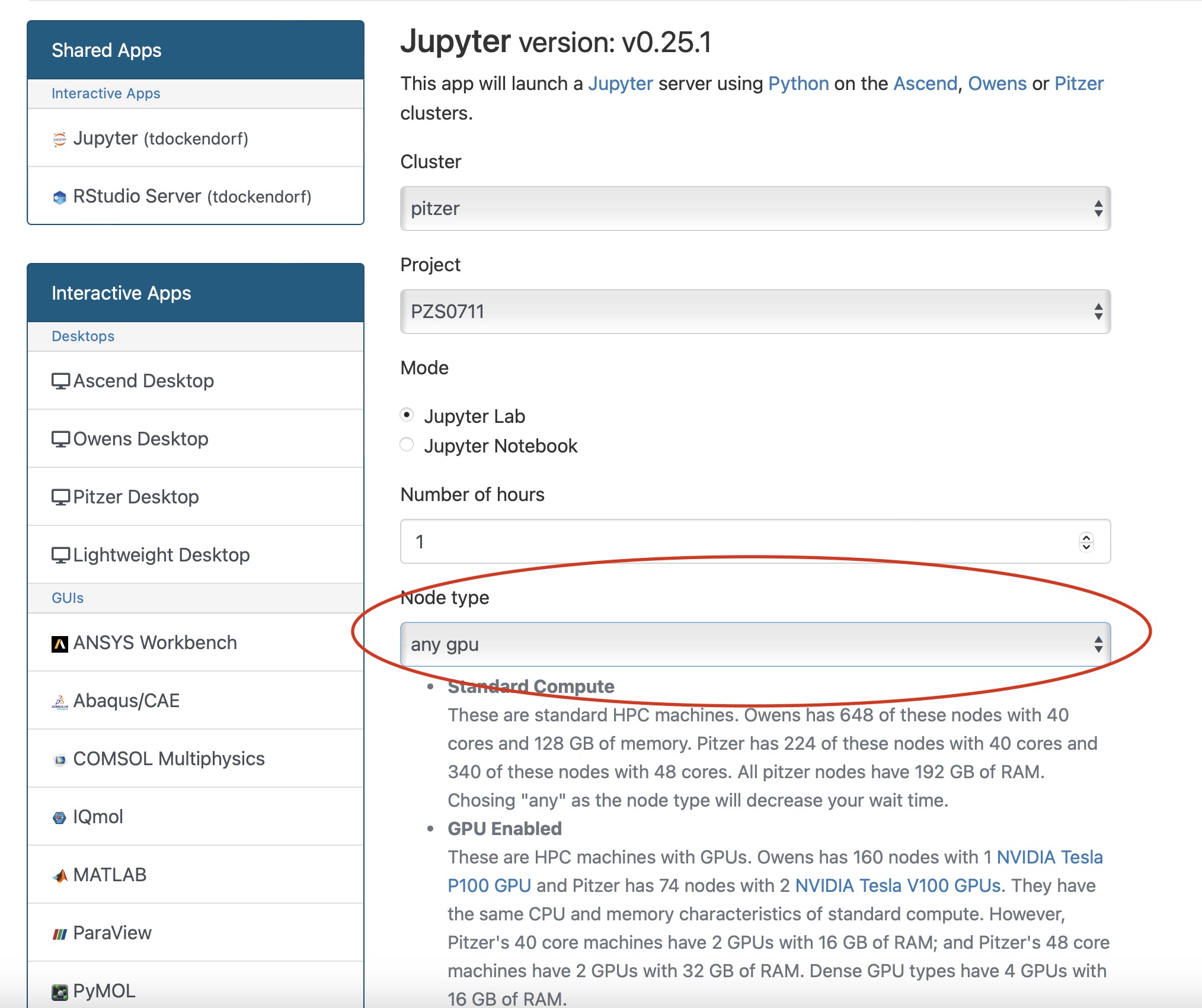
Additional Resources
If you are using Tensorflow, PyTorch or other machine learning frameworks you may want to also consider using Horovod. Horovod will take single-GPU training scripts and scale it to train across many GPUs in parallel.
HOWTO: Use Globus (Overview)

Globus is a cloud-based service designed to let users move, share, and discover research data via a single interface, regardless of its location or number of files or size.
Globus was developed and is maintained at the University of Chicago and is used extensively at supercomputer centers and major research facilities.
Globus is available as a free service that any user can access. More on how Globus works can be found on the Globus "How It Works" page.
Data Transfer
Globus can be used to transfer data between source and destination systems including OSC storage, cloud storage, storage at other HPC centers with Globus support, laptops, desktops.
If you would like to transfer data between OSC storage and your own laptop/desktop which has not installed Globus Connect Personal yet, please go to 'Globus Connect Personal Installation' first
Step 1: Log into Globus
Log into https://www.globus.org/
When prompted to login, select "Ohio Supercomputer Center (OSC)" from the drop-down list of organizations and then click Continue. This will redirect you to the Ohio Supercomputer Center login page where you can log in with your OSC username and password.
Step 2: Locate collections of your data
Click 'File Manager' on the left of the page. Switch to 'two panel' view by click icons next to 'Panels'. One panel will act as the source while the other is the destination.
Click 'Collection' to search the collection of your data.
For OSC storage, use 'OSC endpoints' information to locate the collection.
Step 3: Transfer the file
Select the file(s) or directory that you would like to transfer between collections. You can now select the "Transfer or Sync to..." and hit the blue "Start" icon above the file selector.
Step 4: Verfiy the transfer
Click Activity in the command menu on the left of the page to go to the Activity page.
Globus Connect Personal Installation
Globus Installation on Windows
-
Launch the application installer.
-
If you have local administrator permissions on your machine, and will be the only user, click on 'Install'.
- If you do not have local administrator permissions or wish to specify a non-default destination directory for installation, or will have multiple GCP users, click on the 'Browse' button and select a directory which you have read/write access to.
- If you do not have local administrator permissions or wish to specify a non-default destination directory for installation, or will have multiple GCP users, click on the 'Browse' button and select a directory which you have read/write access to.
-
After installation has completed GCP will launch. Click on 'Log In' in order to authenticate with Globus and begin the Collection Setup process.
-
Grant the required consents to GCP Setup.
-
Enter the details for your GCP Collection.
-
Exit the Setup process or open the Globus web app to view collection details or move data to or from your collection.
-
At the end of the installation, you will see an icon in the menu bar at the bottom of your screen, indicating that Globus Connect Personal is running and your new collection is ready to be used.
OSC endpoints
- Enter 'OSC Globus Connect Server' in the endpoint search box to find all the endpointss managed by OSC as below:
| Endpoint | |
|---|---|
| OSC's home directory | OSC $HOME |
| OSC's project directory | OSC /fs/project |
| OSC's scratch directory | OSC /fs/scratch |
| OSC's ess storage | OSC /fs/ess |
| AWS S3 storage | OSC S3 |
| OSC high assurance |
OSC /fs/ess/ High Assurance for project storage OSC /fs/scratch/ High Assurance for scratch storage |
Note: the default path will be $HOME for home directory, /fs/ess for project storage, /fs/scratch for scratch filesystem. You can change to a more specific directory by providing the path in ‘Directory’. The location for project/scratch data would be under /fs/ess/<project-code> or /fs/scratch/<project-code>.
Data Sharing
With Globus, you can easily share research data with your collaborators. You don’t need to create accounts on the server(s) where your data is stored. You can share data with anyone using their identity or their email address.
To share data, you’ll create a guest collection and grant your collaborators access as described in the instructions below. If you like, you can designate other Globus users as "access managers" for the guest collection, allowing them to grant or revoke access privileges for other Globus users.
-
Log into Globus and navigate to the File Manager.
-
Select the collection that has the files/folders you wish to share and, if necessary, activate the collection.
-
Highlight the folder that you would like to share and Click Share in the right command pane.
Note: Sharing is available for folders. Individual files can only be shared by sharing the folder that contains them. If you are using an ad blocker plugin in your browser, the share button may be unavailable. We recommend users whitelist app.globus.org, docs.globus.org, and globus.org within the plugin to circumvent this issue.If Share is not available, contact the endpoint’s administrator or refer to Globus Connect Server Installation Guide for instructions on enabling sharing. If you’re a using a Globus Connect Personal endpoint and you’re a Globus Plus user, enable sharing by opening the Preferences for Globus Connect Personal, clicking the Access tab, and checking the Sharable box.
-
Provide a name for the guest collection, and click Create Share. If this is the first time you are accessing the collection, you may need to authenticate and consent to allow Globus services to manage your collections on your behalf.
-
When your collection is created, you’ll be taken to the Sharing tab, where you can set permissions. The starting permissions give read and write access (and the Administrator role) to the person who created the collection.
Click the Add Permissions button or icon to share access with others. You can add permissions for an individual user, for a group, or for all logged-in users. In the Identity/E-mail field, type a person’s name or username (if user is selected) or a group name (if group is selected) and press Enter. Globus will display matching identities. Pick from the list. If the user hasn’t used Globus before or you only have an email address, enter the email address and click Add.
Note: Granting write access to a folder allows users to modify and delete files and folders within the folder.You can add permissions to subfolders by entering a path in the Path field.
-
After receiving the email notification, your colleague can click on the link to log into Globus and access the guest collection.
-
You can allow others to manage the permissions for a collection you create. Use the Roles tab to manage roles for other users. You can assign roles to individual users or to groups. The default is for the person who created the collection to have the Administrator role.
The Access Manager role grants the ability to manage permissions for a collection. (Users with this role automatically have read/write access for the collection.)
When a role is assigned to a group, all members of the group have the assigned role.
Data Sharing with Service Account
Sometimes, a group may need to share data uploaded by several OSC users with external entities using Globus. To simplify this process OSC can help set up a service account that owns the data and create a Globus share that makes the data accessible to individuals. Contact OSC Help for this service.
Further Reading
HOWTO: Use AWS S3 in Globus
Beofre creating a new collection, please set up a S3 bucket and configure the IAM access permissions to that bucket. If you need more information on how to do that, see the AWS S3 documentation and Amazon Web Services S3 Connector pages.
Create a New Collection
- Login to Globus. If your institution does not have an organizational login, you may choose to either Sign in with Google or Sign in with ORCiD iD
- Navigate to the 'COLLECTIONS' on the sidebar and search 'OSC S3'. Click 'OSC S3' to go to this gateway
- Click on the “Credentials” tab of the “OSC S3” page. Register your AWS IAM access key ID and AWS IAM Secret Key with Globus. Click the “Continue” button, and you will return to the full “Credentials” tab where you can see your saved AWS access credentials.
- Click on the 'Collections' tab. You will see all of the collections added by you before. To add a new collection, click 'Add Guest Collection'. Click the “Browse” button to get a directory view and select the bucket or subfolder folder you want. Provide the name of the collection in 'Display Name” field
- Click 'Create Collection' to finish the creation
- Click 'COLLECTIONS' on the sidebar. Click the 'Administered by You' and then you can locate the new collection you just created.
HOWTO: User OneDrive in Globus
Accessing User OneDrive in Globus
Globus is a cloud-based service designed to let users move, share, and discover research data via a single interface, regardless of its location or number of files or size.
This makes Globus incredibly useful for transferring large files for users. This service is also able to work alongside OneDrive, making your this storage even more attainable.
Data Transfer with OneDrive
Step 1: Log into Globus
Log into https://www.globus.org/
When prompted to login, select "Ohio Supercomputer Center (OSC)" from the drop-down list of organizations and then click Continue. This will redirect you to the Ohio Supercomputer Center login page where you can log in with your OSC username and password.
Step 2: Choose the Appropriate Collections
Select the File Manager tab on the left hand toolbar. You will be introduced to the file exchange function in the two-panel format.
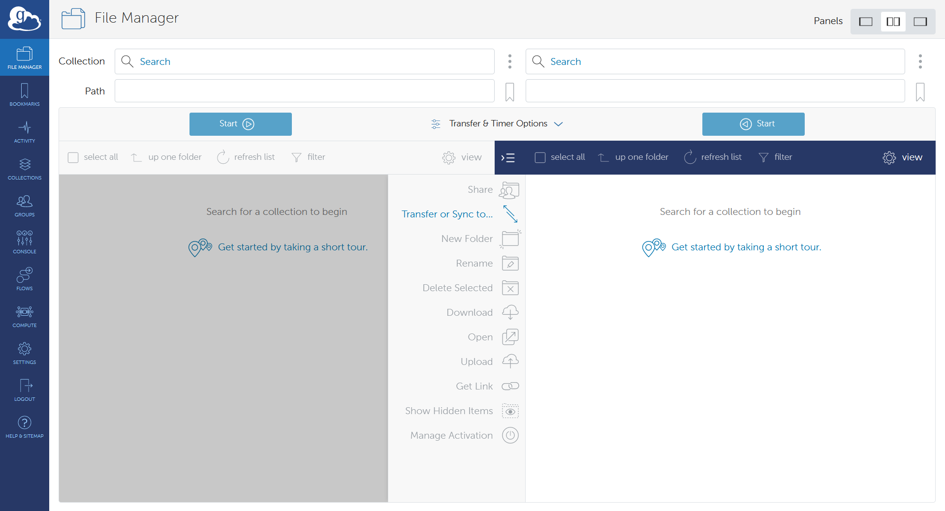
In the left panel, select the collection that you would like to import the data to. In the right panel, you can simply type "OSU OneDrive" or "OSU OneDrive Student" and the collection will appear. Students will need to use their buckeyemail.osu.edu emails in order to access the student OneDrive.
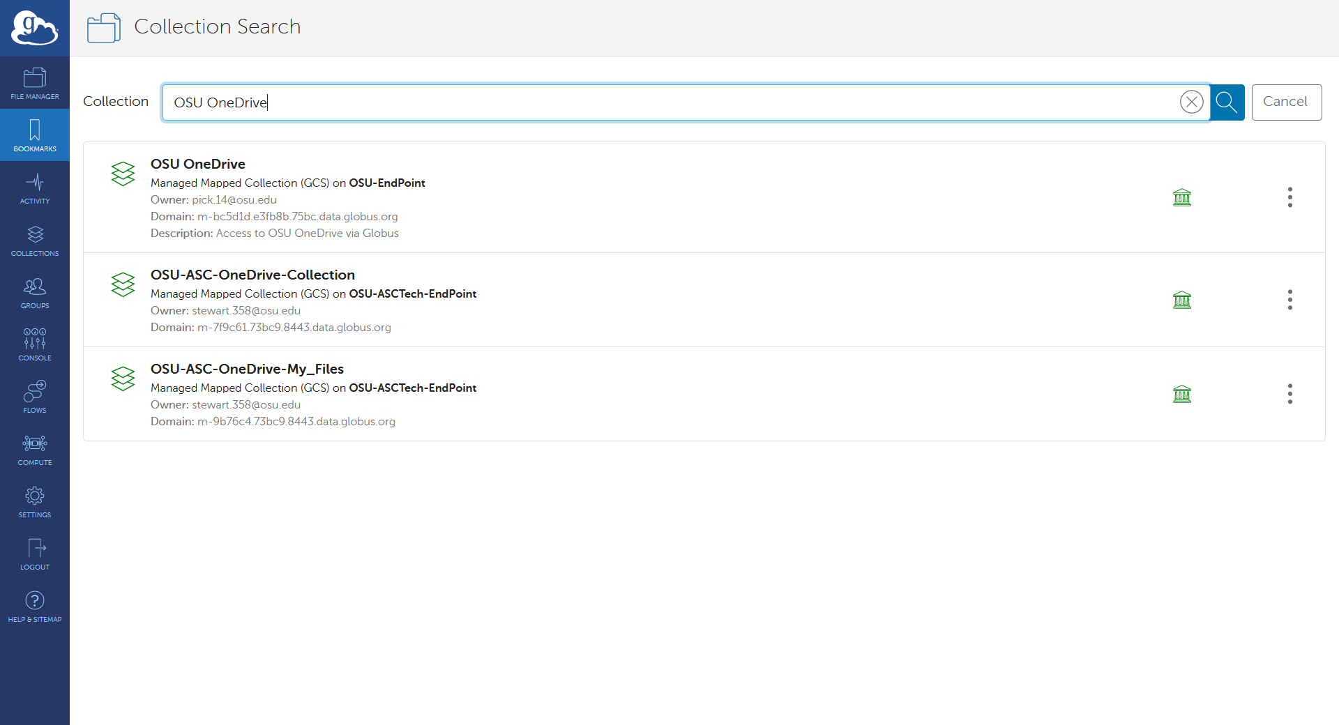
The first time that you access this collection, you will be prompted for some initial account setup.
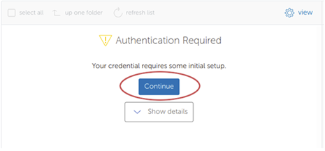
Complete the Authentication Request and, if prompted, verify that you wish to grant access to the Collection.
Once opened, the default location will be My Files. Click the "up one folder" icon to see the other locations.
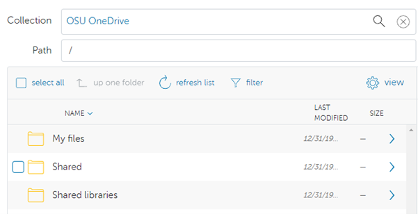
Step 3: Transfer the Files
Select the file(s) or directory that you would like to transfer between collections. You can now select the "Transfer or Sync to..." and hit the blue "Start" icon above the file selector.
Step 4: Verify the transfer
Click Activity in the command menu on the left of the page to go to the Activity page. You will now be able to monitor the processing of the request and the confirmation receipt will appear here.
Following Sites in SharePoint
To follow a SharePoint site, log into the OSU SharePoint service with your OSC name.# credentials. Next, navigate to the site you would like to connect to via Globus and click the star icon on the site to follow:
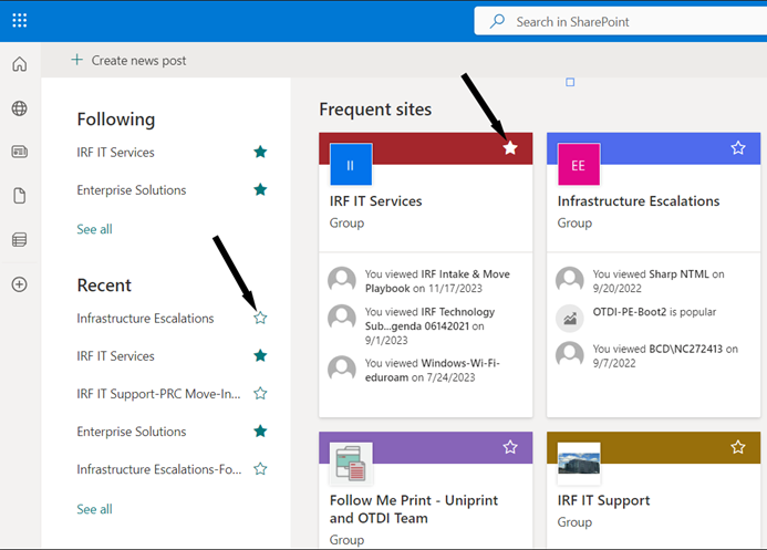
Finally, return to Globus and click the "up one folder" button until you see the "Shared libraries" and the SharePoint site will now be available.
HOWTO: Deploy your own endpoint on a server
OSC clients who are affiliated with Ohio State can deploy their own endpoint on a server using OSU subscriptions. Please follow the steps below:
- Send a request to OSC Help the following information:
- Name of organization that will be running the endpoint, ie: OSU Arts and Sciences
- NOTE: if the name already exists, they will have to coordinate with the existing Admin for that project
- OSU affiliated email address associated with the Globus account, ie: name.#@osu.edu
- Name of organization that will be running the endpoint, ie: OSU Arts and Sciences
- OSC will create a new project at https://developers.globus.org, make the user provided in #1 the administrator, and inform the user to set up the endpoint credentials
- The user goes to https://developers.globus.org/ and chooses “Register a new Globus Connect Server v5”. Under the project, the user chooses Add dropdown and chooses Add new Globus Connect Server. Provide a display name for the endpoint, ie: datamover02.hpc.osc.edu. Select “Generate New Client Secret” and save that value and Client ID and use those values when configuring the Globus Connect Server install on their local system
- The user finishes configuring Globus Connect Server and runs the necessary commands to register the new endpoint with Globus. Once the new endpoint is registered, please email OSC Help the endpoint name so we can mark the endpoint as managed under the OSU subscription
HOWTO: Use VNC in a batch job
SSHing directly to a compute node at OSC - even if that node has been assigned to you in a current batch job - and starting VNC is an "unsafe" thing to do. When your batch job ends (and the node is assigned to other users), stray processes will be left behind and negatively impact other users. However, it is possible to use VNC on compute nodes safely.
You can use OnDemand, which is a much easier way to access desktops. If your work is not a very large, very intensive computation (for example, you do not expect to saturate all of the cores on a machine for a significant portion of the time you have the application you require open - e.g., you are using the GUI to set up a problem for a longer non-interactive compute job), you can choose one VDI under "Virtual Desktop Interface" from "Desktops" menu. Otherwise, please use "Interactive HPC" from Desktops" menu.
The examples below are for Pitzer. If you use other systems, please see this page for supported versions of TurboVNC on our systems.
Starting your VNC server
Step one is to create your VNC server inside a batch job.
Option 1: Interactive
The preferred method is to start an interactive job, requesting an gpu node, and then once your job starts, you can start the VNC server.
salloc --nodes=1 --ntasks-per-node=40 --gpus-per-node=1 --gres=vis --constraint=40core srun --pty /bin/bash
This command requests an entire GPU node, and tells the batch system you wish to use the GPUs for visualization. This will ensure that the X11 server can access the GPU for acceleration. In this example, I have not specified a duration, which will then default to 1 hour.
module load virtualgl
module load turbovnc
Then start your VNC server. (The first time you run this command, it may ask you for a password - this is to secure your VNC session from unauthorized connections. Set it to whatever password you desire. We recommend a strong password.)
vncserver
To set the vnc password again use the
vncpasswd command.The output of this command is important: it tells you where to point your client to access your desktop. Specifically, we need both the host name (before the :), and the screen (after the :).
New 'X' desktop is p0302.ten.osc.edu:1
Connecting to your VNC server
Because the compute nodes of our clusters are not directly accessible, you must log in to one of the login nodes and allow your VNC client to "tunnel" through SSH to the compute node. The specific method of doing so may vary depending on your client software.
The port assigned to the vncserver will be needed. It is usually 5900 + <display_number>. e.g.
New 'X' desktop is p0302.ten.osc.edu:1
would use port 5901.
Linux/MacOS
Option 1: Manually create an SSH tunnel
I will be providing the basic command line syntax, which works on Linux and MacOS. You would issue this in a new terminal window on your local machine, creating a new connection to Pitzer.
ssh -L <port>:<node_hostname>.ten.osc.edu:<port> <username>@pitzer.osc.edu
The above command establishes a proper ssh connection for the vnc client to use for tunneling to the node.
Open your VNC client, and connect to localhost:<screen_number>, which will tunnel to the correct node on Pitzer.
Option 2: Use your VNC software to tunnel
This example uses Chicken of the VNC, a MacOS VNC client. It is a vncserver started on host n0302 with port 5901 and display 1.
The default window that comes up for Chicken requires the host to connect to, the screen (or port) number, and optionally allows you to specify a host to tunnel through via SSH. This screenshot shows a proper configuration for the output of vncserver shown above. Substitute your host, screen, and username as appropriate.
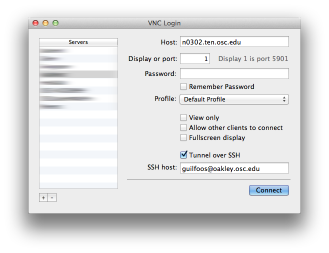
When you click [Connect], you will be prompted for your HPC password (to establish the tunnel, provided you did not input it into the "password" box on this dialog), and then (if you set one), for your VNC password. If your passwords are correct, the desktop will display in your client.
Windows
This example shows how to create a SSH tunnel through your ssh client. We will be using Putty in this example, but these steps are applicable to most SSH clients.
First, make sure you have x11 forwarding enabled in your SSH client.
Next, open up the port forwarding/tunnels settings and enter the hostname and port you got earlier in the destination field. You will need to add 5900 to the port number when specifiying it here. Some clients may have separate boxes for the desination hostname and port.
For source port, pick a number between 11-99 and add 5900 to it. This number between 11-99 will be the port you connect to in your VNC client.
Make sure to add the forwaded port, and save the changes you've made before exiting the configutations window.
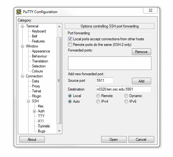
Now start a SSH session to the respective cluster your vncserver is running on. The port forwarding will automatically happen in the background. Closing this SSH session will close the forwarded port; leave the session open as long as you want to use VNC.
Now start a VNC client. TurboVNC has been tested with our systems and is recommended. Enter localhost:[port], replacing [port] with the port between 11-99 you chose earlier.
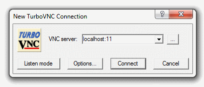
If you've set up a VNC password you will be prompted for it now. A desktop display should pop up now if everything is configured correctly.
How to Kill a VNC session?
Occasionally you may make a mistake and start a VNC server on a login node or somewhere else you did not want to. In this case it is important to know how to properly kill your VNC server so no processes are left behind.
The command syntax to kill a VNC session is:
vncserver -kill :[screen]
In the example above, screen would be 1.
You need to make sure you are on the same node you spawned the VNC server on when running this command.
Service:
Fields of Science:
HOWTO: Use a Conda/Virtual Environment With Jupyter
The IPython kernel for a Conda/virtual environment must be installed on Jupyter prior to use. This tutorial will walk you though the installation and setup procedure.
First you must create a conda/virtual environment. See create conda/virtual environment if there is not already an environment that has been created.
Install kernel
Load the preferred version of Python or Miniconda3 using the command:
module load python
or
module load miniconda3
Replace "python" or "miniconda3" with the appropriate version, which could be the version you used to create your Conda/venv environment. You can check available Python versions by using the command:
module spider python
Run one of the following commands based on how your Conda/virtual environment was created. Replace "MYENV" with the name of your Conda environment or the path to the environment.
-
If the Conda environment was created via
conda create -n MYENVcommand, use the following command:~support/classroom/tools/create_jupyter_kernel conda MYENV
-
If the Conda environment was created via
conda create -p /path/to/MYENVcommand, use the following command:~support/classroom/tools/create_jupyter_kernel conda /path/to/MYENV
-
If the Python virtual environment was created via
python3 -m venv /path/to/MYENVcommand, use the following command~support/classroom/tools/create_jupyter_kernel venv /path/to/MYENV
The resulting kernel name appears as "MYENV [/path/to/MYENV]" in the Jupyter kernel list. You can change the display name by appending a preferred name in the above commands. For example:
~support/classroom/tools/create_jupyter_kernel conda MYENV "My_Research_Project"
This results in the kernel name "My_Research_Project" in the Jupyter kernel list.
You should now be able to access the new Jupyter kernel on OnDemand in a jupyter session. See Usage section of Python page for more details on accessing the Jupyter app.
Install Jupyterlab Debugger kernel
According to Jupyterlab page, debugger requires ipykernel >= 6. Please create your own kernel with conda using the following commands:
module load miniconda
conda create -n jupyterlab-debugger -c conda-forge "ipykernel>=6" xeus-python
~support/classroom/tools/create_jupyter_kernel conda jupyterlab-debugger
You should see a kernelspec 'conda_jupyterlab-debugger' created in home directory. Once the debugger kernel is done, you can use it:
1. go to OnDemand
2. request a JupyterLab app with kernel 3
3. open a notebook with the debugger kernel.
4. you can enable debug mode at upper-right kernel of the notebook
Manually install kernel
If the create_jupyter_kernel script does not work for you, try the following steps to manually install kernel:
# change to the proper version of python
module load python

# replace with the name of conda env
MYENV=useful-project-name

# create the cpnda enironment
conda create -n $MYENV

# Activate your conda/virtual environment
## For Conda environment
source activate $MYENV

# ONLY if you created venv instead of conda env
## For Python Virtual environment
source /path/to/$MYENV/bin/activate

# Install Jupyter kernel
python -m ipykernel install --user --name $MYENV --display-name "Python ($MYENV)"
Remove kernel
If the envirnoment is rebuilt or renamed, users may want to erase any custom jupyter kernel installations.
Be careful! This command will erase entire directories and all files within them.
rm -rf ~/.local/share/jupyter/kernels/${MYENV}
Service:
Fields of Science:
HOWTO: Use an Externally Hosted License
Many software packages require a license. These licenses are usually made available via a license server, which allows software to check out necessary licenses. In this document external refers to a license server that is not hosted inside OSC.
If you have such a software license server set up using a license manager, such as FlexNet, this guide will instruct you on the necessary steps to connect to and use the licenses at OSC.
Users who wish to host their software licenses inside OSC should consult OSC Help.
You are responsible for ensuring you are following your software license terms. Please ensure your terms allow you to use the license at OSC before beginning this process!
Introduction
Broadly speaking, there are two different ways in which the external license server's network may be configured. These differ by whether the license server is directly externally reachable or if it sits behind a private internal network with a port forwarding firewall.
If your license server sits behind a private internal network with a port forwarding firewall you will need to take additional steps to allow the connection from our systems to the license server to be properly routed.
License Server is Directly Externally Reachable
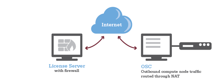
License Server is Behind Port Forwarding Firewall
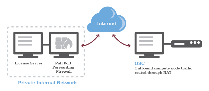
Unsure?
If you are unsure about which category your situation falls under contact your local IT administrator.
Configure Remote Firewall
OSC changed NAT IP addresses on December 14, 2021. Please update the IP addresses of license server configured for the firewall to allow the connections from nat.osc.edu (192.148.249.248 to 192.148.249.251).
In order for connections from OSC to reach the license server, the license server's firewall will need to be configured. All outbound network traffic from all of OSC's compute nodes are routed through a network address translation host (NAT).
The license server should be configured to allow connections from nat.osc.edu including the following IP addresses to the SERVER:PORT where the license server is running:
- 192.148.249.248
- 192.148.249.249
- 192.148.249.250
- 192.148.249.251
A typical FlexNet-based license server uses two ports: one is server port and the other is daemon port, and the firewall should be configured for the both ports. A typical license file looks, for example,
SERVER licXXX.osc.edu 0050XXXXX5C 28000
VENDOR {license name} port=28001
In this example, "28000" is the server port, and "28001" is the daemon port. The daemon port is not mandatory if you use it on a local network, however it becomes necessary if you want to use it outside of your local network. So, please make sure you declared the daemon port in the license file and configured the firewall for the port.
Confirm Configuration
The firewall settings should be verified by attempting to connect to the license server from the compute environment using telenet.
Get on to a compute node by requesting a short, small, interactive job and test the connection using telenet:
telnet <License Server IP Address> <Port#>
(Recommended) Restrict Access to IPs/Usernames
It is also recommended to restrict accessibility using the remote license server's access control mechanisms, such as limiting access to particular usernames in the options.dat file used with FlexNet-based license servers.
For FlexNet tools, you can add the following line to your options.dat file, one for each user.
INCLUDEALL USER <OSC username>
If you have a large number of users to give access to you may want to define a group using GROUP within the options.dat file and give access to that whole group using INCLUDEALL GROUP <group name> .
Users who use other license managers should consult the license manager's documentation.
Modify Job Environment to Point at License Server
The software must now be told to contact the license server for it's licenses. The exact method of doing so can vary between each software package, but most use an environment variable that specifies the license server IP address and port number to use.
For example LS DYNA uses the environment variable LSTC_LICENSE and LSTC_LICENSE_SERVER to know where to look for the license. The following lines would be added to a job script to tell LS-DYNA to use licenses from port 2345 on server 1.2.3.4, if you use bash:
export LSTC_LICENSE=network
export LSTC_LICENSE_SERVER=2345@1.2.3.4
or, if you use csh:
setenv LSTC_LICENSE network
setenv LSTC_LICENSE_SERVER 2345@1.2.3.4
License Server is Behind Port Forwarding Firewall
If the license server is behind a port forwarding firewall, and has a different IP address from the IP address of the firewall, additional steps must be taken to allow connections to be properly routed within the license server's internal network.
- Use the license server's fully qualified domain name in SERVER line in the license file instead of the IP address.
- Contact your IT team to have the firewall IP address mapped to the fully qualified domain name.
Software Specific Details
The following outlines details particular to a specific software package.
ANSYS
Uses the following environment variables:
ANSYSLI_SERVERS=<port>@<IP>
ANSYSLMD_LICENSE_FILE=<port>@<IP>
If your license server is behind a port forwarding firewall and you cannot use a fully qualified domain name in the license file, you can add ANSYSLI_EXTERNAL_IP={external IP address} to ansyslmd.ini on the license server.
HOWTO: Use ulimit command to set soft limits
This document shows you how to set soft limits using the ulimit command.
The ulimit command sets or reports user process resource limits. The default limits are defined and applied when a new user is added to the system. Limits are categorized as either soft or hard. With the ulimit command, you can change your soft limits for the current shell environment, up to the maximum set by the hard limits. You must have root user authority to change resource hard limits.
Syntax
ulimit [-HSTabcdefilmnpqrstuvx [Limit]]
| flags | description |
|---|---|
| -H | Specifies that the hard limit for the given resource is set. If you have root user authority, you can increase the hard limit. Anyone can decrease it |
| -S | Specifies that the soft limit for the given resource is set. A soft limit can be increased up to the value of the hard limit. If neither the -H nor -S flags are specified, the limit applies to both |
| -a | Lists all of the current resource limits |
| -b | The maximum socket buffer size |
| -c | The maximum size of core files created |
| -d | The maximum size of a process's data segment |
| -e | The maximum scheduling priority ("nice") |
| -f | The maximum size of files written by the shell and its children |
| -i | The maximum number of pending signals |
| -l | The maximum size that may be locked into memory |
| -m | The maximum resident set size (many systems do not honor this limit) |
| -n | The maximum number of open file descriptors (most systems do not allow this value to be set) |
| -p | The pipe size in 512-byte blocks (this may not be set) |
| -q | The maximum number of bytes in POSIX message queues |
| -r | The maximum real-time scheduling priority |
| -s | The maximum stack size |
| -t | The maximum amount of cpu time in seconds |
| -u | The maximum number of processes available to a single user |
| -v | The maximum amount of virtual memory available to the shell and, on some systems, to its children |
| -x | The maximum number of file locks |
| -T | The maximum number of threads |
The limit for a specified resource is set when the Limit parameter is specified. The value of the Limit parameter can be a number in the unit specified with each resource, or the value "unlimited." For example, to set the file size limit to 51,200 bytes, use:
ulimit -f 100
To set the size of core dumps to unlimited, use:
ulimit –c unlimited
How to change ulimit for a MPI program
The ulimit command affects the current shell environment. When a MPI program is started, it does not spawn in the current shell. You have to use srun to start a wrapper script that sets the limit if you want to set the limit for each process. Below is how you set the limit for each shell (We use ulimit –c unlimited to allow unlimited core dumps, as an example):
- Prepare your batch job script named "myjob" as below (Here, we request a job with 5-hour 2-cores):
#!/bin/bash
#SBATCH --ntasks=2
#SBATCH --time=5:00:00
#SBATCH ...


...
srun ./test1
...
- Prepare the wrapper script named "test1" as below:
#!/bin/bash
ulimit –c unlimited
.....(your own program)
-
sbatch myjob
Service:
HOWTO: test data transfer speed
The data transfer speed between OSC and another network can be tested.
Test data transfer speed with iperf3 tool
Connect to a data mover host at osc and note the hostname.
$ ssh sftp.osc.edu
# login
$ hostname
datamover02.hpc.osc.edu
# the hostname may also be datamover01.hpc.osc.edu
From there, an iperf3 server process can be started. Note the port used.
iperf3 -s -p 5201
Server listening on 5201
# the above port number could be different
Test Upload Performance
Next, on your local machine, try to connect to the iperf3 server process
iperf3 -c datamover02.hpc.osc.edu -p 5201
If it connects sucessfully, then it will start testing and then finish with a summary
Connecting to host datamover02.hpc.osc.edu, port 5201
...
- - - - - - - - - - - - - - - - - - - - - - - - -
[ ID] Interval           Transfer     Bitrate
[  7]   0.00-10.00  sec  13.8 MBytes  11.6 Mbits/sec                  sender
[  7]   0.00-10.00  sec  13.8 MBytes  11.6 Mbits/sec                  receiver
Test Download Performance
For the data downloaded speed, you can also test the newwork performace in the reverse direction, with the server on datamover02 sending data, and the client on your computer receiving data:
iperf3 -c datamover02.hpc.osc.edu -p 5201 -R
Run iperf3 using docker (alternative)
Docker can be used if iperf3 is not installed on client machine, but docker is.
$ docker run --rm -it networkstatic/iperf3 -c datamover02.hpc.osc.edu -p 5201
Make sure iperf3 server process is running on OSC datamover host or client iperf3 will fail with error.
Citation
The Ohio Supercomputer Center provides High Performance Computing resources and expertise to academic researchers across the State of Ohio. Any paper citing this document has utilized OSC to conduct research on our production services. OSC is a member of the Ohio Technology Consortium, a division of the Ohio Department of Higher Education.
Hardware
OSC services can be cited by visiting the documentation for the service in question and finding the "Citation" page (located in the menu to the side).
HPC systems currently in production use can be found here: https://www.osc.edu/supercomputing/hpc
Decommissioned HPC systems can be found here: https://www.osc.edu/supercomputing/hpc/decommissioned.
Logos
Please refer to our branding webpage.
Citing OSC
We prefer that you cite OSC when using our services, using the following information, taking into account the appropriate citation style guidelines. For your convenience, we have included the citation information in BibTeX and EndNote formats.
Ohio Supercomputer Center. 1987. Ohio Supercomputer Center. Columbus OH: Ohio Supercomputer Center. http://osc.edu/ark:/19495/f5s1ph73.
BibTeX:
@misc{OhioSupercomputerCenter1987,
ark = {ark:/19495/f5s1ph73},
url = {http://osc.edu/ark:/19495/f5s1ph73},
year  = {1987},
author = {Ohio Supercomputer Center},
title = {Ohio Supercomputer Center}
}
EndNote:
%0 Generic
%T Ohio Supercomputer Center
%A Ohio Supercomputer Center
%R ark:/19495/f5s1ph73
%U http://osc.edu/ark:/19495/f5s1ph73
%D 1987
Here is an .ris file to better suit your needs. Please change the import option to .ris.
Documentation Attachment:
New User Training
Transcript:
Kate Cahill
[Slide: “An Introduction to OSC Resources and Services”]
All right, so thank you again for everyone for joining and we'll get started. So today I'm going to give you an introduction to OSC resources and services. So, talking about our systems, and how you can get to use them as a researcher.
[Slide: “Kate Cahill Education & Training Specialist”]
As I said, my name is Kate and I do education and training for OSC.
[Slide: “Outline”]
So today we're going to cover just general, you know, intro to OSC Intro to high performance, computing so some concepts and definitions that are useful to know if you're new to using HPC systems. I'll talk about the hardware that we have at OSC, and then some details on how to get a new account or a new project, if you're starting a new research project with us. We'll take a short break, and then the latter part of the presentation will be about using the system. So, the user environment, how to work with software on the clusters and an intro to batch processing and running jobs on the systems. And then we'll finish. I'll just do a demonstration of our OnDemand web portal, so you can see what that looks like if you haven't logged into it already, and I’ll highlight the features of that, and how that makes it easy to get started. So like I said, you can put questions in the chat. Let me know if you can't hear me, or if something's not clear, and you can also ask questions as we go. I'll pause between our sections.
[Slide: “What is the Ohio Supercomputer Center?”]
So what is the Ohio supercomputer center?
[Slide: “About OSC”]
We are a part of the Ohio Department of Higher Education and we’re part of a group that's called OH-TECH, which is a statewide consortium for technology support services. So OH-TECH is comprised of OSC, OhioLINK, which is the digital library services, and OARnet, which is the the statewide network system that we have. And so, we are a statewide resource for all higher education institutions in Ohio, and we provide, you know, different types of high performance computing services and computational science expertise. And we, you know, are meant to serve the whole State.
[Slide: “Service Catalog”]
So here is some details about the services that we have at OSC. So I’m sure you’re aware that we have, you know, HPC clusters. So, that's the main reason people come to OSC is to use our large-scale computing resources. But we also have other services, such as data storage for different research needs, education activities. So you know, training events like this one, you know we can do training, you know, at your institution or for your department or group. We also partner with people on education projects to use HPC in classes and develop curriculum for computational science of different kinds. And we do a lot of web software development. So we have a team that's focused on developing different types of software and tools to use HPC resources on the web. And that's where we get our OnDemand portal. So that's their main focus. And then scientific software development as well. So, we manage the software that we have on our clusters. But we also partner with people to develop new software optimize existing things to make software run better on HPC systems.
[Slide: “Client Services”]
So, here's just an overview of kind of the activities that OSC was involved in, and this is fiscal year, 22. So this is the end of 2021, and the first half of 2022. So we had 55 active Ohio universities, with projects, 68, Ohio, or 68 companies or industry, part, you know people that were active doing research on our systems, 54 nonprofits and government agencies had active users and then we had other educational institutions with active accounts at OSC. And we have almost 8,500 active clients at this point, so people with accounts who are using our systems. And a 1,000 of those a little more than a 1,000 of those are PIs, so those are people that that run projects and lead research. And you can see the breakdown of roles, you know, for the people that we have accounts for. So about a quarter of them or faculty or staff, and the bulk of them are students. And we had a 127 college courses that used OSC so we have classroom projects that are separate from our research projects, and you can, you know, use those to have your students access OSC and do course work and homework for your courses. Twenty-nine training opportunities such as this one with the over 700 trainees.
[Slide: “HPC Concepts”]
And so that's just a general overview of OSC. Let me know if you have any questions about what we do or any of our services. But now I want to talk about HPC concepts. So, a lot of people who use OSC are new to HPC in general. So I’m just going to talk with generally about some concepts and define some terms.
[Slide: “Why Use HPC?”]
So, there's a lot of reasons why people need to use high performance computing resources. You know, typically people have some analysis or simulation that they want to run, that, you know, if they want to run it at a larger scale, it's just going to take days or weeks on a typical desktop computer. And so, they just need more computing power, so more cores, more ability to parallelize other types of acceleration, like using GPUs, or just using distributed computing tools like Spark. Or it may be that you're working with data sets, or you're collecting data, and it's just a very large volume of data, and it's really hard to work with that, you know, given the storage, or the memory that you have on your own systems. So, we have large memory nodes for that purpose. And then you know, more storage in general so you can work with larger data sets. Or it could be that there's a particular software package that just works best on HPC systems, and you can't access it otherwise.
[Slide: “What is the difference between your laptop and a supercomputer?”]
So here are three general points that it's good to keep in mind about what's the difference between your laptop or desktop and a supercomputer. So one way to think about a supercomputer is thinking about you know thousands or tens of thousands of individual computers that are linked together through a high, a very high-speed network, and so that you know, so you can, you know, link them all together so they can work together to do larger scale computing. That's really how we get the supercomputers. Another thing to keep in mind is that nobody is going to the computer itself. No one is standing in front of the supercomputer and working with it directly through a you know, a monitor and a keyboard. Everybody is remotely connecting to these systems. So they're all you know in in a in a separate, a separate area, you know, and we're all logging into them remotely. And so it's just important to keep in mind that your activity on the system is kind of moderated by the network that you're using. So if you're on a fast network, you know, you're going to get really good integration with what you're doing and really good response rates. If you're on a slower network, if you're, you know, somewhere with a slow wi-fi connection, you're going to see a slower response. So just keep that in mind when you're working with the systems. And then the third point is that these systems are shared. So you saw that, I said we have over almost 8,500 clients active on our systems this past year, and so at any given time hundreds of people are logged on and using the system or running jobs. So there's just some things that we ask you to do, so that we can all use the system, and everyone can have their jobs completed and their research move forward as efficiently as possible. So there's certain things that that the system we have, the system set up in a certain way, so that it can be shared effectively.
[Slide: “HPC Terminology”]
So here's some terminology that's good to know for using HPC systems. So we talk a lot about a node or a compute node. And so a node is sort of the unit of a cluster, and it's it's kind of equivalent to a high end desktop. It has its own memory, it has its own storage, it has its own processors. And so you know, each of those nodes is sort of like a desktop computer, and then they're all linked together, and they create the cluster. And so the compute cluster is that group of nodes that are connected by a high-speed network, and that forms the supercomputer. So, a supercomputer and a cluster, or a about synonymous. And a core we often talk about a core that usually is, relates to a processor or a CPU, and so you'll see I'll explain our hardware in a minute, and I’ll talk about cores per node. So that's really processors CPUs per node. And so, there's usually multiple cores per processor, chip and per node. And so you need to know that architecture when you make a request to the system. And then, finally, we refer a lot to GPUs, and those are graphical processing units. So, this is a separate type of processor that does much more kind of very parallel work. We refer to it often as an accelerator because it it's really good at doing some, you know, a lot of small calculations really, quickly, and so depending on the type of work you have to do, if it can be broken up effectively to use a GPU, it can speed up your work a lot. So GPUs have become very popular in lots of different workflows. So they're a big part of super computers now.
[Slide: “Memory”]
And some of the things to keep in mind memory is the really fast storage that holds the data that is being calculated on. So in an active an active job or simulation or analysis, memory is holding the data that's being used for that analysis. And so in a supercomputer we have memory, that is, you can have shared memory, some memory that's shared across all of your processors on a single node. The memory will be shared for all the processors on that node. If you use more than one node in your calculations then you're going to have distributed memory where the know the memory on one node won't be the same as the memory on the on another node, and you have to make sure that your calculation has all the information it needs. So, there's different types of decisions you have to make about how to use the system to, you know, speed up your code as much as much as possible, taking into account the different memory that's available to you. And each core has an associated amount of memory. So, we don't require that you tell us how much memory you need you just make a node and core request, and then we give you a relative amount of memory associated with that number, of course. But I'll go into more detail with the hardware.
[Slide: “Storage”]
And for storage. So, storage is where you're, you're keeping things for a longer term. Then you would keep you keep data in memory. And so you can have storage that is, you know, active in a in an active job holding, you know, data that's already been created, or it's already been analyzed. And you just need that for your output. And then there's longer term storage, for you know different purposes as well, and I’ll go over our data storage options at OSC.
[Slide: “Structure of a Supercomputer”]
And so here is just a way to look at the supercomputer kind of covering all these concepts. So you can see the compute nodes are labeled at the bottom, and so those are the individual nodes that are network together to form the cluster. So that's the main part of the supercomputer. We have a separate type of node called the login node. That's for just kind of setting up jobs and reviewing output, but not for your main compute. And then you, as the researcher, are accessing this through some kind of network, either using a terminal program or a web portal. And then every and then the data storage options are available, you know, to access through the login nodes and the compute nodes as well.
[Slide: “Hardware Overview”]
So, any questions about general HPC things or General OSC surfaces. So, I'll go on to talk about the hardware that we have at OSC.
[Slide: “System Status”]
So at this point, so right now we have three systems that are currently active, and that's Owens, Pitzer and Ascend, and Pitzer is really divided into two sections. The original Pitzer and Pitzer expansion. So that's what you see here. So, Owens has been around the longest, Ascend just came online at the end of last year. And so, the larger systems are Owens and Pitzer. You can see if you look at the node, count that Ascend is a lot smaller. It's more specialized. So, it's a GPU focused system. So, unless you have work that is really GPU heavy that you need, GPUs, you may not, and you may not Ascend at all. Owens and Pitzer are still our main systems. And then, so yeah, that kind of gives you the general sense of the systems. But now I’m going to talk more specifically about each of them.
[Slide: “Owens Compute Nodes”]
So on Owens, Owens has 648 standard nodes. Those are standard compute nodes, and each of those has 28 cores or processors per node, and 128 GB of memory. So that's a standard compute node on Owens
[Slide: “Owens Data Analytics Nodes”]
Owens also has 16 large memory nodes. Each of those nodes has 48 cores per node and one and a half terabytes of memory, as well as 12 TB of local disk, space or storage. And so those are, for you know the types of jobs that need just a lot of memory to, you know hold all the data that's being, you know, calculated, or to do all the analytics that needs to be done.
[Slide: “Owens GPU Nodes”]
And Owens also, in addition to the regular compute nodes, has a 160 GPU nodes. And so, these are the same as the standard compute nodes so 28 cores per node, but they also have one NVIDIA P100 GPUs on them. So, each node has one GPU.
[Slide: “Owens Cluster Specifications”]
And so here is kind of all those parts of Owens put together. And this may be hard to read. It's not very large. But you can definitely look at all of these details and more specifications on Owens on our main website. If you just go under cluster computing, and you can choose Owens. You can see all these details.
[Slide: “Pitzer Cluster Specifications Original”]
And so here is the overview for Pitzer. So this is the original part of Pitzer. And so this has 224 standard nodes, with 40 cores per node. And 192 GB of memory, and a terabyte of local storage per node. There's also 32 GPU nodes on Pitzer with the same 40 cores per node.
There's more memory, and there's two GPUs per node on Pitzer. So it's depending on the workload you need to you need to run. You might need, you know, two GPUs per note instead of one. And then there are four huge memory notes on Pitzer as well. Those are 80 cores per node and 3 TB of memory. So again, you know, these are for jobs that need a lot of single node parallelization. So you can use a lot of cores on one node, and you need a lot of memory.
[Slide: “Pitzer Cluster Specifications”]
Here we go, and so Pitzer, so the expansion of Pitzer, in addition to the original Pitzer, the expansion has 340 standard nodes, and those each have 48 cores per node. And then 42 GPU nodes as well. And again, those are two GPUs per node. And there's also 12 large memory nodes on the Pitzer expansion as well. And for dense GPU nodes so for jobs that that can take advantage of, for you can use four GPUs per node we have a couple of nodes for that as well. And again, the details of this are on our website. That's where you can see all of the technical specifications for our clusters.
[Slide: “Ascend Cluster Specifications”]
And so Ascend like I said, it's the newest system. It's much smaller in in sort of node counts than Owens or Pitzer and so it's mainly focused on GPU nodes. So Ascend has 24 GPU nodes, with 88 total cores per node and 4 GPUs per node as well. So yeah, like, I said, this is GPU focused system. So, if your if your work is going to be, you know, very GPU heavy you can request access to the system, but we didn't give general access to everyone because it's not very large, and it's kind of specialized.
[Slide: “Login Nodes - Usage”]
And just to reiterate the login nodes. So, each of the systems has login nodes, and so that's when you first log into the system you're on the login nodes. And so, this is where you will set up your files, edit files, you know, get your input data and everything together to submit a job to the batch system so that you can access the compute nodes. This is not where you're going to run your jobs. There's very small limits on the login nodes as to how long any process can run, so if you start a process of some kind, it'll get stopped after 20 min. And you only have access to 1 GB of memory on the login nodes. So, they're really not for compute that you can do some small scale work, you know, like opening a graphical interface, or compiling like a very small code as long as it's really, you know not very compute intensive and won't take very long. But you don't want to use it too much, because it can slow down the login notes for everybody else. So the login nodes are mainly for setting up your jobs and looking at output, not for actually computing. And that's why we want you to use the batch system to use the compute nodes.
[Slide: “Data Storage Systems”]
So now I’m going to talk about our data storage systems. Any questions?
[Slide: “File Systems at OSC”]
So we have several file systems that OSC for different purposes. I'm going to talk about four of them. So, you can see them here on the data storage on the left. We have the home file system, the project file system, the scratch file system, and then the compute nodes. So, the storage that's available on the compute nodes. Those are the ones that I’m going to focus on.
[Slide: “Research Data Storage”]
And so the some of the features of these different file systems, the home location. So every account, so if you have an account at OSC, you'll have a location that that's your home directory, and that'll be on the home file system. And most accounts will have 500 GB storage available in the home directory. There might be some accounts that that have less, but almost all of them will have the 500 GB, and this is the main place that we expect that you can use to store your files, and we back this up regularly. So if you happen to lose something, or accidentally delete something vital, you can let us know, and we can help you restore it. So, we consider this kind of permanent protected storage. And then but if your group or your project needs more storage, then is available in each of the user accounts, then the project PI can request access to the project file system. And so this is just like a supplemental storage to the home directories. Most PIs or most groups need about one to 5 TB of storage on the project file system, and it's accessible to everybody in that project. And then there's also the scratch file system available. And this is available to everyone, you don't have to request access, so you can access it directly, and this is, we consider temporary storage. So we don't back up the scratch file system so you can use it, for you know large files that you might not want to fill your home directory up with. You can put them there if you're going to be actively using them, for you know, a couple of weeks or months, and you just want to keep them, you know, somewhere else than your Home Directory. That's what the scratch file system is for. And then on the compute nodes each compute node that you'll have access to will have its own storage. And so it's for use during your job. And so ideally, all of your compute. And you know, file creation, file, generation output, creation will happen on the compute node, and then at the end of the job you'll just copy everything back to your home directory. So you're not, you know, using the network to during your job to read and write. It just makes your job more efficient kind of reduces the overhead of that of that network usage, but you only have access to it while your job is running. So at the end of the job, you all that information is removed. So you said to make sure to copy back your results at the end of your job. We also have archive storage. So if you have some data set or database that you want to have, you know, stored for a longer period of time. They're not going to access regularly. You can talk to us. You can email OSC help and ask about that as well.
[Screen: Table showing Filesystem, Quota, Network, Backed-Up?, Purged]
And so here's just kind of an overview of the different features of the file systems. So, and I've included on the on the left. So the name of the file, the file system is home. You can use the variable dollar sign home as a reference to your home directory for the project file system. It's FSESS or FS Project, I think it's just FSESS. And then your project code to reach your project files. If you have that as a separate request the scratch file system you can reach by FS scratch, and then your project code, and then you can reference the location of the compute. Compute node storage with the TMPDIR and you can see the quotas so generally the quota for the home directory is a half terabyte. The project file system is you know amount that you choose. That's by request. We have a nominal quota of a 100 TB on the scratch file system and the compute. The compute file system varies, but it's usually at least 1 TB per node. You can see the different network speeds for the file system. So like I said, the home and the project or not very fast, the scratch file system has a faster network. So that is, you know, if you wanted to keep a large data set on the scratch file system and use it during a job. The scratch file system is more optimized for that. The home and project are backed up, scratch and compute are not. And we do have a purge on the scratch file system about every 90 days, so that is, if you have some files out there that you haven't used in a while, you know if they're you know. If they get old, they haven’t been they haven't been access for 90 days, they might be purged. We don't always purge, but when it gets full, we do, and then the compute node file system is removed when your job ends, so you only have access to it while your job is running. And again, there's links here on the bottom about where you can get more details about the file systems.
[Slide: “Getting Started at OSC”]
And I see information question in the chat. But sounds like you got the information you needed. So any other question, any questions about file systems or hardware?
Olamide E Opadokun:
Yeah. So the other file types that are backed up, for how long are they kept on the system?
Kate Cahill:
So you mean, like in the Home Directory?
Olamide E Opadokun:
Yeah.
Kate Cahill:
So there's a couple of layers to that. So Wilbur, do you know what our current scheme is for that? I know we back it up like multiple times a day, but then we have offsite backups as well. So I think it might be up to two weeks, or maybe further.
Wilbur Ouma:
Yeah, I don't have the correct, all the information on that. Yeah. But I know we do back up almost several times per day. Yeah, but we've had some requests people coming back that maybe they inadvertently deleted some files or data, maybe the last, you know a month or several weeks, and we've been able to recover those.
Kate Cahill:
Yeah, so I would certainly say that if you, if you do find that something has been deleted that you want recovered to let us know as soon as possible, because, you know, we don't keep them, you know, for months back, or anything. So you don't want it to wait too long. But at least couple of weeks, I believe.
Olamide E Opadokun:
Okay. So they kept on the system for a couple of weeks and then deleted?
Kate Cahill:
So the backups. So it's, you know we take. We take backups of the home directories, and we can restore things that have been deleted from a from an earlier version. And then we have offsite backups as well. So if we, if we happen to have some problem with our system and we lose power, we have versions that are stored off site as well. It's just a question of kind of like, how long those like you how far back those backups go. But yeah, so it's more about, you know. If you if you remove something and then you want it back, we can restore an earlier version of it. Once you let us know that you need it again. But on the home directory and the project directory we don't remove anything, so it's entirely up to you what's on those.
Olamide E Opadokun:
Oh, okay, so that that's not what subjected to the long-term storage, the archive storage, because that's just always going to be available right?
Kate Cahill:
Yeah. So the archive storage is a separate storage. So it's not like we automatically archive your home directory. That would be, you’d have to ask us to put something on the archive storage. It would be separate.
Olamide E Opadokun:
Okay, thank you.
Michael Broe:
So the issue, I often I advise graduate students who are working with PIs, who have. So the PI has the OSC account, and then they move away. They go to different jobs that if they go. And so then they ask me, can I get access to my data again? And I'm just would like to clarify if the PI doesn't keep this under control. How long will the data hang around, or how can they access it. If and so they've moved on from the OSU. And so, they no longer have an OSU account and they're trying to get access to data from, maybe several years ago, because their papers just been published. I know it's a big issue, a difficult issue. But I just like to clarify what is going on there.
Kate Cahill:
Yeah. So when someone leaves OSU and is no longer active their account. So I mean, if like, if they're not, if they're not part of your group anymore, and you're not working with them. And you don't, you know you're not going to have them on your OSC account. You know their OSC account will kind of just sort of age. It doesn't get automatically removed, but it goes into a restricted state, and then it goes into an archive state, and we remove that home directory. So it's always a good idea when somebody is leaving, so like, you know, for the PI to make a backup of that of that students' information at OSC so they have access to it if they need something from an earlier project. But yeah, certainly, after a couple of years, and I don't think that we could, that we would still have the student’s home directory data available unless there was some, you know, archive process that we actually said, “Put this on an archive.” I think from our perspective it's up to the PI, the person that runs the project to, you know, make a backup of that information. So, they have it like, make it back up way from OSC.
Michael Broe:
Yeah, or the if they believe the project is going to continue it, it's on the project. It's going to be backed up in, as long as the project exists.
Kate Cahill:
Right, so, if so, yeah, if the student has data in their home directory that everybody else wants to have access to for the project to continue, they should move it to the project directory. That's the shared space between all of the accounts that will stay as long as long as the OSC, the overall project is still there. So, if you have that project that shared project space for everybody in your in your group. You can, you can use that as another way to keep that that information available to everybody else. But yeah, it's definitely something that has to be kind of, there has to be a procedure when somebody leaves to make sure that that data isn't lost.
Michael Broe:
Yes, great, that's the perfect answer. Thank you.
Kate Cahill:
Alright great, so I’m going to start to talk about how to get started at OSC. So, this is more about getting an account and getting a project, and how we manage those things here.
[Slide: “Who can get an OSC Project?”]
So we have different types of projects that are available. So our main type of project is the academic project. And so that's generally led by a PI, and that person is generally a full-time faculty, member or research scientist at an Ohio academic institution. They could also. That's the main type of PI that we have at OSC for academic projects. And so the PI can request a project, and once they have that project, they can put anybody on it that they want, so they can authorize accounts for, you know, students post docs, other faculty, other their staff collectors, people from out of state people from out of the country. Anybody can have an account. But the PI has to have a certain role at an Ohio institution. Another type of project that we have is the classroom project, and so those are for specific courses. So, they're shorter-term projects that are kind of you know, specialized for giving students in a class access to OSC. We also have commercial projects available as well, so commercial organizations can purchase time at OSC as well.
[Slide: “Accounts and Projects at OSC”]
So a project we define a project code. So when you request a new project we'll define a code it becomes with a P, usually has three letters and four numbers, and that is like, I said, headed by a PI and includes any number of other users that the PI authorizes. And this is, and the project is the is how we account for computing resources. An account is a specific user so that will have a specific username and password. And that's how that that person will access OSC systems and the HPC systems. And so, an account is one person. So every person should have a unique account. You can work on more than one project, but you'll just have the one account to access all of them.
[Slide: “Usage Charges”]
And so we do charge for usage of our systems, and those charges are in terms of core hours, GPU hours, and terabyte months. And so, a project will have a dollar balance and any services that you use like compute and storage are charged to that balance and you know we are still subsidized by the state, so our charges are still partially subsidized, and so they're cheaper than your, you know commercial cloud resources. You can see more details on the link here. And yeah. So, if you're interested in in sort of the charges, the specific charges.
[Slide: “Ohio Academic Projects”]
So for academic projects annually, each project can receive a $1,000 grant so that can be your budget for the year, and so that that rolls over every fiscal year. So it'll be the beginning of July. You know, all academic projects will be eligible for a new $1,000 grant and so that's a way to kind of, you know, have a starting budget, and you know, get to use OSC resources, fully subsidized. If you think you're going to need more than that, then you have to add money to that budget. And so we do it this way, so that there are no unexpected charges. So you don't have some, you know, jobs that are over running, you know, or you know that somebody submits too many jobs or they're too big, and they end up charging more. The budget is a hard limit, and we also don't do proposal submissions anymore. We used to have an Allocations Committee that would review proposals, but we don't have that now, since we have this this fee model. The classroom projects that I mentioned before are fully subsidized, so they will have a budget as well. But it is not a budget that will be charged to anyone. And all of these the projects and getting an account are all available at our client portal site which is my.osc.edu.
[Slide: “Client Portal- my.osc.edu”]
And so the client portal, like I said, is mainly for project, management and account management. It's really useful for PIs to kind of oversee the projects, the activity on their projects, so you can. When you log into the client portal. If you're on a project, you'll see some statement about the usage on your projects. So, you can see it broken down by project, by type and system, by usage per day, and then below you'll see your active projects, and then you'll see your budget balance and your usage. So, it's just a way to see that information at a glance, and then you can, you know using the client portal, you can create an account. Keep your email and your password updated. Recover access to your account, if it's restricted, change your shell if you don't want to use the standard batch shell you can change to a different shell, and then you can do things like, manage your users, and request services and resources like storage and software.
[Slide: “Statewide Users Group (SUG)”]
And so OSC, you know, has a statewide users group. So that's you know everybody that uses OSC to give you a chance to provide advice to OSC. So we can hear from the OSC community about. You know what they would like to see OSC do in future kind of where you want to see us go as far as resources or services. So this this group meets twice a year, and there's a chairperson elected yearly from the you know, Ohio Academic community generally, and we have some standing committees that meet as part of this group. So there's Software and Activities Committee and the Hardware and Operations Committee. And this is usually a day long sort of symposium that happens at OSC. But it's also a hybrid event where you can also share your research in poster sessions and Flash talks and meet other OSC researchers. And this happens twice a year, generally April and October. And you can check the OSC calendar to find out information about the next one, which is on April 20th. You can register, you know, present a poster send a flash talk, or just, you know, come and meet OSC staff and other researchers.
[Slide: “Communications & Citing OSC”]
So as far as communications we do send regular user emails, information about downtimes and any other unplanned maintenance events. We do have quarterly downtimes. We just had a downtime yesterday, so we're good for a quarter now. But we want to keep you updated. So make sure your email is is correct so you can receive those. And there's also information on our main website about citation. So if you are gone publish any work you've done with OSC resources, you can. You can cite the resource that you use
[Slide: “Short Break”]
All right, so we're going to take just like a five min break right here, so everybody can get up and move around a little bit, and we'll be back at 1:50. But does anybody have any questions? All right so I’ll be back in five minutes.
[Slide: “Short Break” beginning at about 41:35]
All right, so I’m going to get started again. Does anybody have any questions?
[Slide: “User Environment”]
So now we're going to talk about what it's like to use the systems and some information about HPC systems and software batch system environment.
[Slide: “Linux Operating System”]
So the user environment we use. We have a Linux operating system which is the most widely used in HPC so that's really common. If you have use HPC systems before you've probably interacted with the Linux system. It generally has been a command line based. So you need to have, you know some sense of the commands that you need to enter, to do things like, you know, refiles or move files. There is a choice of shells I mentioned. So bash is the default shell. But there are other shells available. If you you know, want to work at a different shell, you have to change your shell in the client portal. And so then you'll have that environment. And this is open-source software and there's a lot of tutorials available online. We have a couple linked here under the command-line fundamentals page on our website, just as suggestions potential tutorials. It's good to have some command line, comfort like. Just know a couple of standard commands to navigate the file system, for example. Just so you're comfortable in it, but you don't necessarily need to use the command line for most of your work anymore.
[Slide: “Connecting to an OSC Cluster”]
So to connect to an OSC cluster you have a couple of options like I said, everybody connects over a network. So you're going to use some kind of, you know. But you know, network connection tool. The historical way to connect to a system is using ssh through a terminal window. So in a Mac or Linux system you'd open the terminal program, and at the prompt enter ssh and then your user ID and @. And then the name of the sort of address of the system that you want to access. So you could access Owens it'd be owens.osc.edu and SSH. Is the command for secure shell. So you're connecting, you know, to the system through a secure shell. If you have a windows system, I believe there's a terminal program on there now, or you can download some free versions like putty is a terminal program you could use other options for connecting. So the main way that most of OSC clients, the connections, clusters these days is our on Demand portal. So that's our web portal. So you just need a you know you have a browser, and you just need to go to ondemand.osc.edu and enter your OSC user name and password, and then you have access to all the compute resources at OSC. Through the through the browser.
[Slide: “Transferring Files to and from the Cluster”]
Another key step you generally have to take with transferring files. You know you have to take in your set up. Your research is to transfer files to and from the cluster. And so again, you have several options with the command Line tools. You can use sftp or scp, you know, in a terminal window. And so you would, you know. copy either from your local system to the cluster or the other way for smaller files. You can do that right through the login nodes so same kind of connection as the ssh, you can do owens.osc.edu. If your network is slow or your files are larger. You have another option called the file transfer server. So, instead of connecting to Owens or Pitzer directly, you would connect to sftp.osc.edu, and that just gives you access to the same file systems. But you're over a file transfer network that gives you a longer time to transfer file, so there's no time out on there. And so that helps with large files for slow networks. On the OnDemand portal. We have file management tools that include file transfer tools, so you can do a drag and drop to transfer files or use the upload and download buttons and the limit on that. It can be up to 10 GB. That's for very fast networks, so you can get, you know, fairly good size files to transfer again. It's network dependent. So you may see different outcomes depending on where you're connecting to the systems. We also have a tool called globus, and that is for large files or for large file trees. So if you want to transfer a bunch of structure, you know file structure all at once. Globus is another tool for that, and that is a web-based tool as well. It's a not an OSC tool it's a separate tool that we have an account with and you have to set it up once hyou have that it'll transfer files in the background for you and there's how to here Link on the bottom to show you how to get started using globus.
[Slide: “OSC OnDemand”]
So I see a question. Can you access the HPC resources through a terminal? If you don't have an OSU account. So you don't have to have anything to. You know we we're not. We're not a high of state focus, so it's not OSU account. You do have to have an OSC account. So you have to have an account with us at OSC, and you have to have access, you have to have a project, you know that you're a part of that will give you access to the clusters, so you can go to our client Portal, which is my.osc.edu, and you know, get, you know, just create your own OSC account. But until you're on a project you're part of a project, or you've created a project that you're a part of. You won't have cluster access until then. So those are the things you need. And so here's some more details about our on demand portal. So like I said, it's ondemand.osc.edu and you can just open a browser window, and then you just need your OSC username and password to log in you can. You can do a kind of a connection, and then use a different credential. But you still need an OSC account, so you need to know an OSC username and password. And so, once you connect through the OnDemand portal you'll see tools like file management and job management, visualization tools and virtual desktop tools and interactive job apps for different types of things like MATLAB and R and Ansys, so it's pretty comprehensive. It's also a shell window, so you can open a shell and work at the command line as well.
[Slide: “Using and Running Software at OSC”]
So now I want to talk about using software at OSC. And how you get information about it, and how you get started working with it. So any question, any other questions about environment getting logged in? All right so software at OSC.
[Slide: “Software Maintained by OSC”]
Last time I checked which maybe out of date now we had over 235 software. Packages that we maintain at OSC for for our clients. And so there's a lot of lot of options out there. And so, if there's software that you're interested in, you can always so that the first thing you should do is check if we already have it on OSC. So you can check on our main site. You can look under resources and look at available software. And you can browse just a list of all the software or the list by, you know, by cluster or by software type. Or you can just do a search for the software package you're interested in. If we have it, if we support it, we'll have a software page on it, and the software page is really going to give you all the information you need about how you know what you need to know to use the software at OSC. So this will include version information, license information, and some usage examples. So it's really key for forgetting the information to get started.
[Slide: “Third party applications”]
We have, you know, the general programming software tools, various compilers. We have some parallel profilers and debuggers. So if you're writing your own code, you can use these tools to kind of optimize it, Ansys, we have MPI libraries, we have Java, Python, R. These are some of our most popular software packages. We also have parallel specific programming software. So the MPI libraries, OpenMP, CUDA, OpenCL and OpenACC for different types of parallelism for GPU computing and things like that.
[Slide: “Access to Licensed Software”]
So what software licensing is really complicated. But we try, when we support software at OSC to get statewide licenses for academic users as kind of our you know, base level of software access. And so we try and make that, you know, kind of the goal for all of our software, some software, even with that, as the license requires that individual people who are going to use it sign a license agreement. So check the software page it will tell you the details about what the license is, and if you have to take any steps because if you have to sign a license agreement, you can use the software until you've done that and we've added you to the software group. So check the software, page to get information about the license licensing, and if there's any requests you have to make of us. And also, like I said, the software page will have details about how to use the software. So some software also requires that you like put it into your batch script that you are like checking out a license. So you know, specifics like that, you'll see on the software page
[Slide: “OSC doesn’t have the software you need?”]
If we don't support the software that you need. So if you want to use software that that we don't have installed, and we don't maintain. If it's a commercial software package, you can make a request to OSC that you think it this should be included, because you think there's a group of researchers who would use it. So it's about kind of how important it would be to you know a certain number of researchers. We can consider it and add it if it if it seems reasonable. If it's open source, software you know something that you can download yourself. You can install it in your home directory. So that's something that that you can do, so that you and your group members can use that software and we have a how to on kind of the steps that you would take to install as to in software locally, and certainly the you know, whatever software you'd want to install would probably have details that you'd have to read up on to see, you know what the steps are for installing it. And then, if you have a license to, you know, for a commercial software that we support, or you know we can install. We can help you use that license at OSC as well. So there's several options for, software and we can definitely answer any questions about. You know software usage as you as you're trying things.
[Slide: “Loading Software Environment”]
So once you know the software that you want to use. We use software modules to manage the software environments so that we can maintain the software, you know, in a specific location, make updates, add new versions without you having to change all of your paths for the you know location of that software. You can just load the software module into your environment, and then you have access to all the software executables and libraries and things. So you need to use commands like module list. We'll give you the list of software modules that you have loaded already in your environment. So there are some default ones that everybody gets to begin with, and you can always change those. But we kind of have a standard environment that works for most people. So these are like these are command line tools. But you also are going to use these in in the batch scripts that you are going to create. So you should know these. If you want to search for modules, you can do module spider, and then a keyword or module avail. And then, when you want to add software to your environment, you do module load, and then the name of the software, and if there's multiple versions, you may have to be more specific about the version of the module that you want. And you can unload. You can remove things with the module unload, and you can swap versions of software with the module swap command.
[Slide: “Batch Processing”]
So now we can talk about batch processing. Now that we have kind of all the all the pieces.
[Slide: “Why do supercomputers use queuing?”]
So the batch system is the main way to access the compute nodes on the clusters. And so that's kind of the main, I mean part of the system. So you need to know about the batch system so that you can get access to that computing ability. And so supercomputers use queuing so that you can provide all the information to the scheduler and the resource manager, and say, “I need this much of the system. So I need five nodes for six hours, and you know, and here's all the information about my job.” And so the system can take that information, and you know, with everybody else's requests. You end up in a queue, and once the resources are available, then your job will get access to the compute resources, and then it can run all the commands that you've included and do your analysis, and then you get your output. And OSC uses Slurm for scheduler and resource manager. If you're familiar with those so that's the tool that you should become comfortable with.
[Slide: “Steps for Running a Job on the Compute Nodes”]
And that's what we'll see. I'll show you an example batch script using the Slurm commands. And so here's just the steps that you'll go through to run a job to access. The compute nodes. You're going to create a batch script. You're going to prepare and gather your input files in in your home directory or your project directory. But wherever you are with your batch script, that's where your input files will be. You'll submit the job to the to the scheduler. The job will be queued. Once the resources are available, your job will run, and then your results will be copied back into your home directory when your job finishes.
[Slide: “Specifying Resources in a Job Script”]
And so the resources that you have to specify in a job script. I've mentioned them, you know, a couple of times. You need to and specify a number of nodes number of cores per node. Request GPUs, if you want GPUs, you don't have to specify memory, so memory will be relative to the number of cores your request, so it's about 4 GB of memory per core. On the standard nodes. It's different on the on the large memory nodes. But there's still a relative amount. So you don't have to request memory while time is. How long you want to have access to those compute nodes. And so you want to have enough time for your job to complete, but not too much more than that, just because you're when you're requesting more resources than you need, and it will take longer for your job to start. So you do want to overestimate slightly. So you know, if your job is going to take 12 hours. You might want to request, you know, 14 or 16, just to make sure that your job is, you know, fully completed before the wall time ends. And this is something you get used to, you know. You just keep making requests and seeing how long your job really takes, and you get better at getting that wall time, you know. Request to be pretty close to your job needs. You include your project code. So that's how we account for usage. So we need to have that project code in there. And then if there are any software licenses that you have to request. You'll see on the software page. If the license, if the software you want to use has a license request, you have to include that'll be in your job script, too.
[Slide: “Sample Slurm Batch Script”]
And so here is what a sample batch script looks like. So the lines on the top are all are all directly, you know, information to the scheduler, so Slurm has to run in in the batch shell. So we put that bash call in there at the beginning and then all the S batch lines are lines to the schedule, or, you know, these are our specific comments that are directed at the scheduler. And so this includes the wall time. So this is a one hour request number of nodes is two, and n tasks per node is 40. So Slurm uses in tasks per node for cores. So this is two nodes, 40 cores. We give the job a name so that you can recognize it in the in the queue. The account is your project code. So Slurm calls project account, and so you put your project code there and then the rest of the job script are all the commands to run your job. So we just say, you know, make sure that we're starting in the in the directory where our job was submitted. Just so, because that's where our input files should be. So that that line CD Slurm: submit the IR that's just saying, make sure I’m in this directory and then we're going to set up the software environment. So we have a module load command. Then we're going to copy our input files over to the compute node. So the copies CP is copy, hello.c is our code, and we're copying it over to the compute node. And then we're going to so then we're going to run that. We're going to compile our code and then run that that job, get our results and then copy those results. The last line is a copy results, and then back to your working directory. So these are all the commands that we go into a batch script. And so this would be, you, you know, create this as a text file and give it a name and save it.
[Slide: “Submit & Manage Batch Jobs”]
And so, once you have that ready and your input, files are ready. You're going to use this command on the top S batch, and then the name of that job script to submit. If it works and it submits correctly, then you'll see a response, and it's right here, submitted job response,
Slurm response, submitted batch job and you'll get a code. And that is your job ID and that's a way you can reference that job in to the queue. So if you find that you made a mistake in your job script or something, you want to cancel that job you do S cancel and then that job ID so this code here if you wanted to pause your job or hold it before it starts to wait for something else to finish you can use S control hold in the job ID, S control release job ID will release the job from hold. And then if you just want to look at the all the jobs you've submitted. You can do the SQ Command dash you, and then your user ID and that'll just show you what jobs you have in the queue at this point, and what their status is. You want to do that because that that the queue will be very, very long, and if you look at the whole thing, it won't really normally get much information out of it. So this is just kind of the very simple, simple information to get started submitting back jobs to a lot more information you could use to kind of make your jobs more complex or do more things with the batch system. We have several pages on our main website under batch processing at OSC. That have more details about all the different ways. You can use the batch jobs, and Wilbur teaches a training that is the batch system training to have more practice with the batch jobs so you can do some hands-on activities. And so that's another good option.
[Slide: “Scheduling Policies and Limits”]
And so we do have scheduling policies and limits for our systems. And so this is just so that you know jobs don't take over the whole system, or you know. So we have limits both on wall time. So we have for a single node job a wall time limit of 168 hours. For more than one to node jobs. We have a limit of 96 hour, and then we have per user and per group limits. So with number of concurrently running jobs is limited, and the number of processor cores is limited. So if you have many, you know so several large jobs you're limited in the total number of cores you can have in use. And so we have per user and per group. This is the, these are the current limits for Owens. They're not the same from system to system. So if you are curious, you can see those details in the cluster technical specification documents. You'll see a batch limit page that'll kind of give you these details, but you shouldn't unless you or your group are running many, many jobs you probably won't hit these limits.
[Slide: “Waiting for Your Job To Run”]
So how long it takes your job to run is based on how busy the system is, and what kind of resources you request. So if the system is really busy, it'll take longer for your job to start if you request resources that are more limited, like large memory nodes or GPUs, or particular software licenses that are popular. It'll just take longer for those resources to become available. And so I’ll show you on OnDemand how you can see what the system load looks like, so you can kind of if you, if you can, you know, choose which system to use. You can look at the system, load and see which one might start sooner.
[Slide: “Interactive Batch Jobs”]
You can also do batch jobs, interactive batch jobs, where you make a request. You get access to a compute node, and you use it. Live so you can do this from the command line. You can do this through OnDemand. And so this is useful for kind of small scale testing or you know, kind of work flow development, type activities where you want to kind of do things live and see how it goes before you, you know, submit a batch job that runs on its own. And so it's the same kind of you still have to use the batch system so you're still making a request to the resource manager and scheduler number of nodes, number, of course, wall time and then you get access to a compute. No, directly you want to, you know, keep in mind that a large request will take some time to start, and you have to be there when the job starts to use the compute node, because the wall time will start running as soon as the job begins. So this is a useful tool, and OnDemand a lot of interactive tools you can use with different software packages. But this isn't really where you should be doing most of your production work. This is more for testing and trying things out.
[Slide: “Batch Queues”]
Customers have separate batch systems. So if you submit a job to Pitzer, you can't see it in the queue for Owens. So just make sure that you know which system you're submitting to. We do have some debug, some debug reservations on our clusters as well. So if you run a very short job that you just want to test some part of your work. You can use the debug queue to run that quickly.
[Slide: “Parallel Computing”]
To use, you know the systems to get the most you know out of using the systems. You want to use multiple processors. You want to take advantage of the compute resources available. And so you know, that could be multiple cores and a single node. So you know, we have a lot of single notes that are 40 cores, 48 cores, that's a lot of processing just on a single node. That's a good place to start with parallelism to make sure that your job can take advantage of multiple cores and then you can, if you want, you can expand beyond a single core to multiple nodes. And you you're going to use, you know, different types of parallel tools for that to work. So, you have to learn more about MPI. And so, it depends on the type of work you're doing, you know, if you could take advantage of the different types of parallelism.
Michael Broe:
[Slide: “To Take Advantage of Parallel Computing”]
Can I just jump in here? Go ahead. This is Michael Broe. So use showed in a Slurm script before, like number of nodes. Let's say it's one, and then in tasks equals one.
[Slide: “Sample Slurm Batch Script”]
Yeah. Those two in tasks per node equals 50. But there's another Slum option which is CPUs per task. And I don't understand how that interact with tasks per node, and what your recommended procedure is with that.
Kate Cahill:
So I have not used that variation in Slurm. So CPUs per tasks, have you done that Wilbur?
Wilbur Ouma:
No, I haven't, but I have an idea of what it could be doing. So by default, Slurm doesn't equate the number of tasks to be same as the number of CPU cost that we using. So there's some pipeline in which you assign one task. So in Slurm the one tasks actually changes a lot. You could be doing, if you doing an MPI process, it could be the parent task, and then you have like the child tasks, you can have one parent Slurm task that it's running other child tasks that you can say, you know, that will be using different CPUs. So, to simplify things. What you've been like always see is to equate one Slurm task by default to be like one process right? But Slurm still comes with the option of specifying CPUs. Right so, and the reason is because Slurm differentiates CPU calls or processes from tasks like being one. But you just try to simplify that and make sure that okay to make it simple. You will put one processor or one process to be equivalent to one Slurm task. So for most of the analysis that that I do carry out. I don't need to specify the number of CPU, so the like the CPU option for Slurm. I just specify the number of tasks per node or number of tasks, if I'm requesting for one node. And that will by default translate to the number of process that I want for that particular analysis. Does that answer your question, Michael?
Michael Broe:
Yes, it does. I mean if I can ignore CPUs per task completely, I will. I just wanted to know if I was missing something. But if that's if it's a refinement, and it sounds like it's a very great refinement. It's not for this webinar, but it's good to know that what your default take on it is. So that's great. Thank you.
Kate Cahill:
[Slide: “To Take Advantage of Parallel Computing”]
And so yeah, when you're thinking about your parallelism. Make sure that the software you're using, or the code that you're writing is going to take advantage of multiple cores and or multiple nodes. So you want to make sure that that you know you have something that can run in parallel and that you learn about the parallel versions of software that you may already use. We have a tool called mpiexec. That's when you want to use multiple nodes and divide the work across them we use, for you know, so you can use the mpi tools it won't, miss, you know it's not necessarily going to work to just request more. No nodes or cores and it and your job will instantly run faster. You know, if you if it doesn't take advantage of those resources, it's not going to improve anything. So just keep that in mind and do some research on the tools you want to use, and how they work in parallel. So what information you need to know, to provide them so that they can work in parallel.
[Slide: “New – Online Training Available!”]
And so that is kind of everything I wanted to cover about the details about, you know, using OSC resources and then in a minute I'll switch over to a web browser and just show you OnDemand, so you can see what it looks like, but wanted to highlight a couple of things about how to get help and more information. We have some new online training resources available. So this is on ScarletCanvas. So we've got a version of ScarletCanvas from Ohio State. That is an OSC you know version of ScarletCanvas and so this is a free and available to everyone, not OSU, not Ohio State related and all you need to do is create a ScarletCanvas account, and then you can register. You can self register and go through these training courses. And so these are, you know, covers a lot of the material that I covered today, you know, in the OSC Intro, and then the batch system at OSC course we'll cover a lot of but Wilbur covers in his intro to OSC Batch. And so you can look, watch videos go through activities, do quizzes. Do some hands on, just to give you more practice, or a way to give you a reference for these services kind of get comfortable with some of the things, some of the concepts that we've talked about. And you can let us know if there's a certain, you know, certain type of training you'd like to see that we could develop for this as well. So we want to add some new things to this as we go and you can find that if you go to osc.edu, search for training. You get our training page, and you'll get the link for these courses.
[Slide: “Resources to get your questions answered”]
Other resources to get your questions answered. We have a getting started guide, so that I’ll just kind of give you information about different parts of the OSC resources that you can, you know, find information on our website. We have an FAQ that's useful to kind of check into before you, you know. Look for help elsewhere. See if see if that's already included in there. We have a lot of how to's. So these are sort of step by step, guides for doing different activities that people tend to need to do on OSC systems like installing software or installing R or Python packages or using Globus. So there's a lot of those. And then we do have office hours. So there every other Tuesday, and they're virtual so anybody can attend. We do ask you sign up in advance, so you can see them on our website on the event page. There's you know, an event for each one, but make sure you sign up in advance to reserve a time and then we do provide to some updates through the message of the day, which is when you log into our systems, you'll see a big statement, and that's the message of the day, and then we have a twitter feed called HPC notices, and that's just for system updates. So if you follow that you can get any updates we want to share about the systems.
[Slide: “Key OSC Website”]
And these are the main websites that I've talked about today. Our main page is OSC.EDU, our client Portal is MY.OSC.EDU and our web portal to access the clusters is ONDEMAND.OSC.EDU. And so any questions I’m going to switch over to the browser and open OnDemand.
[Switching to Browser]
But thank you for attending. If you, if you want to go before I start the demo go right ahead.
[ondemand.osc.edu browser]
And so I was already logged in. But you just have to log in with your you with your OSC username and password. And then you reach the OnDemand dashboard, and you can see here, here's the message of the day and so you can see some information about, you know updates on Pitzer and general updates about classroom support. Over on the right, you can see we have a separate version of OnDemand that's specific for classroom projects, and that's class.osc.edu. So if you wanted to use OSC for a class you would, we could set up that environment for your class, so it'll so little more simplified and a little more targeted to classroom type users. But also you see some efficiency reports here. So we have some monitoring tools that we use that can tell you kind of how efficient your jobs are, so you can get a sense of sort of when you run a job. Are you using all the resources that you requested, or how efficient is your request? It's just a reference, just so. You kind of have an idea and then on the top here all the different menus for OnDemand. So we have our file manager. And so this will have the different locations that you have access to, so everybody will have a home directory. And then, if you have a scratch location for one, for a project that you'll see that or a project location and you can see the different project codes. So if you have multiple projects, you'll see different locations. If you click on any of your locations and you'll see this sort of file manager open up, and so then you can navigate into your folders. You can create directories or folders.
[Open OnDemand Browser showing File Page then File Example then File Page]
You can create files. You can upload and download and just manage your files. And you can also edit files here so pick one that might be good, so you can, you know, just view the contents of a file. You can edit a file so it can open it as a file editor and make changes to the file and then save them. And then, you know work with files, you know, through this. So you don't, you don't have to go to the command line. You can use this to manage and update and edit files. And so the jobs menu. This is where the job composer is a tool for submitting jobs. So it kind of helps you manage all the parts of creating a job like getting your input files together, creating a job, a job script. The active jobs are, that's just the queue. So once you submitted a job, you can look at jobs that are running. And so over. Here are some filter options, so you can look at your jobs, you can look at all jobs and you can focus on a particular cluster.
[Open OnDemand Browser Active Jobs Page]
So if I look at all jobs on Owens, I can filter this, you know, so I have running jobs. I can look at. I can't spell. I can look at. You know jobs that are in a cued status. But one thing I wanted to show you is when your job is running, you'll be able to get some information about it while it's running. So if you click on the little arrow on the side. You'll get information about the job, so you'll see kind of the job ID. You'll see the requests this is one node 28 cores, the time limit, how long it's been running. But you also see these sort of detailed information about CPU and memory usage, so this can be useful to somebody trying out some new jobs to see, you know, if I make a request of a certain number of cores, is my job actually using all that resource. And so you can see this job is using, you know, about 20 of its CPU usage. And you know not much memory here, but you can get a sense of what your job is doing when it's using the resources. So that's a useful tool. Under the clusters menu, this is where you can open a shell window as a shell, you know terminal window, so you can, you know, use this to work in the command line. There's also a system status tool here, and this is what I mentioned.
[Open OnDemand Browser Cluster Status Page]
If you were, you know, wanted to choose which system to use. The system status can kind of give you a sense of how busy the different clusters are, so that this one is Ascend. And so you may not, you may not have access to a send or may not need to use it, but you can see on Owens. It's about, you know, 70% full. And there's 164 jobs queued. Pitzer is partially offline right now, so even though it says it's not full. It's actually you know at full as far as what's available, so you can see that a lot more jobs are queued on Pitzer right now. So if you wanted to start a job now Owens might be a good option if you can use Owens.
[Open OnDemand Browser Active Jobs Page]
And so that's just the system status, and then the interactive apps are here. And so these are all tools that we've developed at OSC to use these different software packages for data analysis, visualization. You got Jupiter notebooks, Jupiter Lab, Jupiter with Spark and R studio.
[Open OnDemand Browser RStudio Server]
And so each of these are interactive jobs. So you're going to get access to a compute node. And so then you can, you know, use a tool that you may already be familiar with, to run on the compute nodes. Still, these are going to be fairly small scale, but it's a good way to get started. And so you just need to have information like what cluster you want to use, what version of our you want to work with. You have to put in your project code and you tell it how long you want your job to go, and then, if you want to use a specific node type, you can use a GPU node or a large memory node. But just remember, these are interactive job requests, so it's going to wait in the batch until these resources are ready. So if you, if you make a specialized request, it'll take longer, and then you can tell it number, of cores. And so when you launch this, it will once it once the job starts. So I've submitted this and so it's queued in the, you know it's waiting in the queue right now. And so once it starts I’ll open it, and it'll look like our studio, and I’ll have access to my files that are on the system, and I can, just, you know, run, run in R like I would if I was, you know, running on my laptop. But I’m using the compute resources at OSC. So this might take a while to start, because I choose Pitzer. Oh, it looks like it's starting. So it takes a minute to get started. And so now it's running, so I’ll click, connect to R studio and so that it'll just run R studio for me on Pitzer.
[Webpage running R studio via Pitzer]
And so then I, you know. So this is a good way to use the system to kind of get comfortable with running things. But again, this is not necessarily the best choice for production running. You still want to submit, you know, a job to run on the batch system kind of on its own. So you don't have to manage it directly.
[Previous Open OnDemand and R Studio Browser]
And so yeah, you can see other options over here. These are virtual desktops. So just another way to work in the system. You get a virtual Linux desktop, and then these are different graphical interfaces for different visualization and analysis tools. And Jupiter notebooks, like I said, is here. So that's really popular for classroom purposes. And that's those are the main features of OnDemand. So any questions?
Michael Broe:
Thank you very much. That's fantastic introduction. I have a question, but it's not a newbie question. It's about quarto and python. But if I can, you know, explain why you here? I will. But I don't want to get in the way of anything you want to finish up now.
Kate Cahill:
Sure. So I see a question. Do we have to be proficient in R to use OSC system or is the code generated automatically. So you do. I mean, if you want to use R you have to, you know, use some existing R code, or write your own. Wilbur is actually, you know, kind of one of our key R experts. But yeah, the code doesn't get generated automatically. You'd have to create some or use some existing code to do some to do some analysis with R. We do have some R tutorials in here as well. So, I don't know if you saw that when I was doing the interactive app. There is access to OSC tutorial workshop materials. And so that's just, it just gets copied into your home directory, and you can look at some R tutorial tools, so it's just example R code that you can work with. But it's pretty, general. It's just to kind of get you started.
[Previous Open OnDemand Cluster Status Webpage]
So any other questions, if not, thank you for attending and definitely let us know if we can help at any point.
Terry Miller:
Quick question. Are you going to make available these slides?
Kate Cahill:
Yeah. So I I’ll send everybody who registered an email with the slides and the recording. So you can have access to that. And then, like I said, the ScarletCanvas courses cover a lot of this material, too. So it's another way, you could refer back to it, or work through it, or share it with anybody that that you think would benefit.
Terry Miller:
Okay, thank you. I enjoyed your presentation.
Kate Cahill:
So any other questions? So, Michael, let's talk about Python.
Michael Broe:
So I stuck link into the chat that shows that within R studio you can now access Python code. And I teach a course for introduction to computation and biology and most people know.
OSC Custom Commands
There are some commands that OSC has created custom versions of to be more useful to OSC users.
OSCfinger
Introduction
OSCfinger is a command developed at OSC for use on OSC's systems and is similar to the standard finger command. It allows various account information to be viewed.
Availability
| owens | PITZER |
|---|---|
| X |
X |
Usage
OSCfinger takes the following options and parameters.
$ OSCfinger -h
usage: OSCfinger.py [-h] [-e] [-g] USER

positional arguments:
  USER

optional arguments:
  -h, --help   show this help message and exit
  -e           Extend search to include gecos/full name (user) or
               category/institution (group)
  -g, --group  Query group instead of users

Query user:
    OSCfinger foobar

Query by first or last name:
    OSCfinger -e Foo
    OSCfinger -e Bar

Query group:
    OSCfinger -g PZS0001

Query group by category or insitituion:
    OSCfinger -e -g OSC
View information by username
The OSCfinger command can be used to view account information given a username.
$ OSCfinger jsmith
Login: xxx                                   Name: John Smith
Directory: xxx                               Shell: /bin/bash
E-mail: xxx
Primary Group: PPP1234
Groups:
Project Information by Project ID
The OSCfinger command can also reveal details about a project using the -g flag.
$ OSCfinger -g PPP1234
Group: PPP1234                                    GID: 1234
Status: ACTIVE                                    Type: Academic
Principal Investigator: xxx                       Admins: NA
Members: xxx
Category: NA
Institution: OHIO SUPERCOMPUTER CENTER
Description: xxx
---
Search for a user via first and/or last name
If the username is not known, a lookup can be initiated using the -e flag.
This example is shown using the lookup for a first and last name.
$ OSCfinger -e "John Smith"
Login: jsmith                                     Name: John Smith
Directory: xxx                                    Shell: /bin/bash
E-mail: NA
Primary Group: PPP1234
Groups: xxx
Password Changed: Jul 04 1776 15:47 (calculated)  Password Expires: Aug 21 1778 12:05 AM
Login Disabled: FALSE                             Password Expired: FALSE
---
One can also lookup users with only the last name:
$ OSCfinger -e smith
Login: jsmith                                      Name: John Smith
Directory: xxx                                    Shell: /bin/bash
E-mail: NA
Primary Group: PPP1234
Groups:
---
Login: asmith                                     Name: Anne Smith
Directory: xxx                                    Shell: /bin/bash
E-mail: xxx
Primary Group: xxx
Groups:
---
Only the first name can also be used, but many accounts are likely to be returned.
$ OSCfinger -e John
Login: jsmith                                     Name: John Smith
Directory: xxx                                    Shell: /bin/bash
E-mail: xxx
Primary Group: PPP1234
Groups:
---
Login: xxx                                        Name: John XXX
Directory: xxx                                    Shell: /bin/bash
E-mail: xxx
Primary Group: xxx
Groups:
---
Login: xxx                                        Name: John XXX
Directory: xxx                                    Shell: /bin/ksh
E-mail: xxx
Primary Group: xxx
Groups:
---
...(more accounts below)...
Slurm usage
While in a slurm environment, the OSCfinger command shows some additional information:
$ OSCfinger jsmith
Login: xxx Name: John Smith
Directory: xxx Shell: /bin/bash
E-mail: xxx
Primary Group: PPP1234
Groups:
SLURM Enabled: TRUE
SLURM Clusters: pitzer
SLURM Accounts: PPP1234, PPP4321
SLURM Default Account: PPPP1234
It's important to note that the default account in slurm will be used if an account is not specified at job submission.
Service:
OSCgetent
Introduction
OSCgetent is a command developed at OSC for use on OSC's systems and is similar to the standard getent command. It lets one view group information.
Availability
| owens | PITZER |
|---|---|
| X |
X |
Usage
OSCgetent takes the following options and parameters.
$ OSCgetent -h
usage: OSCgetent.py [-h] {group} [name [name ...]]

positional arguments:
  {group}
  name

optional arguments:
  -h, --help  show this help message and exit

Query group:
    OSCgetent.py group PZS0708

Query multiple groups:
    OSCgetent.py group PZS0708 PZS0709
View group information
The OSCgetent command can be used to view group(s) members:
$ OSCgetent group PZS0712
PZS0712:*:5513:amarcum,amarcumtest,amarcumtest2,guilfoos,hhamblin,kcahill,xwang
View information on multiple groups
$ OSCgetent group PZS0712 PZS0708
PZS0708:*:5509:djohnson,ewahl,kearley,kyriacou,linli,soottikkal,tdockendorf,troy
PZS0712:*:5513:amarcum,amarcumtest,amarcumtest2,guilfoos,hhamblin,kcahill,xwang
Service:
OSCprojects
Introduction
OSCprojects is a command developed at OSC for use on OSC's systems and is used to view your logged in accounts project information.
Availability
| owens | PITZER |
|---|---|
| X |
X |
Usage
OSCprojects does not take any arguments or options:
$ OSCprojects
OSC projects for user amarcumtest2:

Project         Status          Members
-------         ------          -------
PZS0712         ACTIVE          amarcumtest2,amarcumtest,guilfoos,amarcum,xwang
PZS0726         ACTIVE          amarcumtest2,xwangtest,amarcum
This command returns the current users projects, whether those projects are active/restricted and the current members of the projects.
Service:
OSCusage
Introduction
OSCusage is command developed at OSC for use on OSC's systems. It allows for a user to see information on their project's usage, including different users and their jobs.
Availability
| owens | PITZER |
|---|---|
| X | X |
Usage
OSCusage takes the following options and parameters.
$ OSCusage --help
usage: OSCusage.py [-h] [-u USER]
                   [-s {opt,pitzer,glenn,bale,oak,oakley,owens,ruby}] [-A]
                   [-P PROJECT] [-q] [-H] [-r] [-n] [-v]
                   [start_date] [end_date]

positional arguments:
  start_date            start date (default: 2021-03-16)
  end_date              end date (default: 2021-03-17)

optional arguments:
  -h, --help            show this help message and exit
  -u USER, --user USER  username to run as. Be sure to include -P or -A.
                        (default: amarcum)
  -s {opt,pitzer,glenn,bale,oak,oakley,owens,ruby}, --system {opt,pitzer,glenn,bale,oak,oakley,owens,ruby}
  -A                    Show all
  -P PROJECT, --project PROJECT
                        project to query (default: PZS0712)
  -q                    show user data
  -H                    show hours
  -r                    show raw
  -n                    show job ID
  -v                    do not summarize
  -J, --json Print data as JSON
  -C, --current-unbilled   show current unbilled usage
  -p {month,quarter,annual}, --period {month,quarter,annual}   Period used when showing unbilled usage (default:   month)
  -N JOB_NAME, --job-name JOB_NAME
                        Filter jobs by job name, supports substring match and
                        regex (does not apply to JSON output)
Usage Examples:

    Specify start time:
        OSCusage 2018-01-24

    Specify start and end time:
        OSCusage 2018-01-24 2018-01-25

    View current unbilled usage:
        OSCusage -C -p month
Today's Usage
Running OSCusage with no options or parameters specified will provide the usage information in Dollars for the current day.
$ OSCusage
----------------  ------------------------------------
                  Usage Statistics for project PZS0712
Time              2021-03-16 to 2021-03-17
PI                guilfoos@osc.edu
Remaining Budget  -1.15
----------------  ------------------------------------

User          Jobs    Dollars    Status
------------  ------  ---------  --------
amarcum       0       0.0        ACTIVE
amarcumtest   0       0.0        ACTIVE
amarcumtest2  0       0.0        ACTIVE
guilfoos      0       0.0        ACTIVE
hhamblin      0       0.0        ACTIVE
kcahill       0       0.0        ACTIVE
wouma         0       0.0        ACTIVE
xwang         12      0.0        ACTIVE
--            --      --
TOTAL         12      0.0
Usage in Timeframe
If you specify a timeframe you can get utilization information specifically for jobs that completed within that period.
$ OSCusage 2020-01-01 2020-07-01 -H
----------------  ------------------------------------
                  Usage Statistics for project PZS0712
Time              2020-01-01 to 2020-07-01
PI                Brian Guilfoos <guilfoos@osc.edu>
Remaining Budget  -1.15
----------------  ------------------------------------

User          Jobs    core-hours    Status
------------  ------  ------------  ----------
amarcum       86      260.3887      ACTIVE
amarcumtest   0       0.0           ACTIVE
amarcumtest2  0       0.0           RESTRICTED
guilfoos      9       29.187        ACTIVE
hhamblin      1       1.01          ACTIVE
kcahill       7       40.5812       ACTIVE
wouma         63      841.2503      ACTIVE
xwang         253     8148.2638     ACTIVE
--            --      --
TOTAL         419     9320.681
Show only a single user's usage
Specify -q to show only the current user's usage. This stacks with -u to specify which user you want to see.
$ OSCusage -u xwang -q 2020-01-01 2020-07-01 -H
----  -------------------------------
      Usage Statistics for user xwang
Time  2020-01-01 to 2020-07-01
----  -------------------------------

User    Jobs    core-hours    Status
------  ------  ------------  --------
xwang   253     8148.2638     -
--      --      --
TOTAL   253     8148.2638
Show a particular project
By default, the tool shows your default (first) project. You can use -P to specify which charge code to report on.
$ OSCusage -P PZS0200 -H
----------------  ------------------------------------
                  Usage Statistics for project PZS0200
Time              2020-09-13 to 2020-09-14
PI                David Hudak <dhudak@osc.edu>
Remaining Budget  0
----------------  ------------------------------------

User        Jobs    core-hours    Status
----------  ------  ------------  ----------
adraghi     0       0.0           ARCHIVED
airani      0       0.0           ARCHIVED
alingg      0       0.0           ARCHIVED
You can show all of your charge codes/projects at once, by using -A .
Select a particular cluster
By default, all charges are shown in the output. However, you can filter to show a particular system with -s .
$ OSCusage -s pitzer -H
----------------  ------------------------------------
                  Usage Statistics for project PZS0712
Time              2021-03-16 to 2021-03-17
PI                guilfoos@osc.edu
Remaining Budget  -1.15
----------------  ------------------------------------

User          Jobs    core-hours    Status
------------  ------  ------------  --------
amarcum       0       0.0           ACTIVE
amarcumtest   0       0.0           ACTIVE
amarcumtest2  0       0.0           ACTIVE
guilfoos      0       0.0           ACTIVE
hhamblin      0       0.0           ACTIVE
kcahill       0       0.0           ACTIVE
wouma         0       0.0           ACTIVE
xwang         0       0.0           ACTIVE
--            --      --
TOTAL         0       0.0
Changing the units reported
The report can show usage dollars. You can elect to get usage in core-hours using -H or raw seconds using -r
$ OSCusage 2020-01-01 2020-07-01 -r
----------------  ------------------------------------
                  Usage Statistics for project PZS0712
Time              2020-01-01 to 2020-07-01
PI                Brian Guilfoos <guilfoos@osc.edu>
Remaining Budget  -1.15
----------------  ------------------------------------

User          Jobs    raw_used    Status
------------  ------  ----------  ----------
amarcum       86      937397.0    ACTIVE
amarcumtest   0       0.0         ACTIVE
amarcumtest2  0       0.0         RESTRICTED
guilfoos      9       105073.0    ACTIVE
hhamblin      1       3636.0      ACTIVE
kcahill       7       146092.0    ACTIVE
wouma         63      3028500.0   ACTIVE
xwang         253     29333749.0  ACTIVE
--            --      --
TOTAL         419     33554447.0


Detailed Charges Breakdown
Specify -v to get detailed information jobs.
You can add the -n option to the -v option to add the job ID to the report output. OSCHelp will need the job ID to answer any questions about a particular job record.
Please contact OSC Help with questions.
Service:
OSC User Code of Ethics
The Ohio Supercomputer Center (OSC) exists to provide state-of-the-art computing services to universities and colleges; to provide supercomputer services to Ohio scientists and engineers; to stimulate unique uses of supercomputers in Ohio; to attract students, faculty, resources and industry; to catalyze inter-institutional supercomputer research and development projects; to serve as the model for other state-sponsored technology initiatives.
OSC serves a large number and variety of users including students, faculty, staff members, and commercial clients throughout the state of Ohio. Ethical and legal standards, in particular, that apply to the use of computing facilities are not unique to the computing field. Rather, they derive directly from standards of common sense and common decency that apply to the use of any public resource. Indeed, OSC depends upon the spirit of mutual respect and cooperative attitudes.
This statement on conditions of use is published in that spirit. The purpose of this statement is to promote the responsible, ethical, and secure use of OSC resources for the protection of all users.
Authorized Use
As a condition of use of OSC facilities, the user agrees:
- To respect the privacy of other users; for example, users shall not intentionally seek information on, obtain copies of, or modify files, tapes, or passwords belonging to other users unless explicitly authorized to do so by those users.
- To respect the legal protection provided by copyrights and licenses to programs and data; for example, users shall not make copies of a licensed computer program to avoid paying additional license fees.
- To respect the intended usage for which access to computing resources was granted; for example, users shall use accounts authorized for their use by the principal investigator responsible for these accounts only for the purposes specified by the principal investigator and shall not use any other user's account.
- To respect the integrity of computing systems; for example, users shall not intentionally develop or use programs that harass other users or infiltrate a computer or computing systems or damage or alter the software components of a computing system.
- To respect the financial structure of computing systems; for example, users shall not intentionally develop or use any unauthorized mechanisms to alter or avoid charges levied by OSC for computing services.
- To not enable other institutions or users to avoid licensing restrictions or fees by simply allowing them to use their account.
- To abide by software specific licensing terms and restrictions, as outlined in the specific software page or agreement.
In addition, users are expected to report to OSC information that they may obtain concerning instances in which the above conditions have been or are being violated.
Violations of the following conditions are certainly unethical and are possibly a criminal offense: unauthorized use of another user's account; tampering with other users' files, tapes, or passwords, harassment of other users; unauthorized alteration of computer charges; and unauthorized copying or distribution of copyrighted or licensed software or data. Therefore, when OSC becomes aware of possible violations of these conditions, it will initiate an investigation. At the same time, in order to prevent further possible unauthorized activity, OSC may suspend the authorization of computing services to the individual or account in question. In accordance with established practices, confirmation of the unauthorized use of the facilities by an individual may result in disciplinary review, expulsion from his/her university, termination of employment, and/or legal action.
Users of computing resources should be aware that although OSC provides and preserves the security of files, account numbers, and passwords, security can be breached through actions or causes beyond reasonable control. Users are urged, therefore, to safeguard their data, to take full advantage of file security mechanisms built into the computing systems, and to change account passwords frequently.
Appropriate Use
Computing resources shall be used in a manner consistent with the instructional and/or research objectives of the community, in general, and consistent with the objectives of the specified project for which such use was authorized. All uses inconsistent with these objectives are considered to be inappropriate use and may jeopardize further authorization.
Beyond the allocation of computing resources, OSC normally cannot and does not judge the value or appropriateness of any user's computing. However, the use of computing resources for playing games for purely recreational purposes, the production of output that is unrelated to the objectives of the account, and, in general, the use of computers simply to use computing resources are examples of questionable use of these resources.
When possible inappropriate use of computing resources is encountered, OSC shall notify the principal investigator responsible. The principal investigator is expected either to take action or to indicate that such use should be considered appropriate.
Should possible inappropriate use continue after notification of the principal investigator, or should unresolvable differences of opinion persist, these shall be brought to the attention of OSC staff for recommendations on further action. Upon the recommendation of OSC staff, the Director may impose limitations on continued use of computing resources.
Responsible Use
Users are expected to use computing resources in a responsible and efficient manner consistent with the goals of the account for which the resources were approved. OSC will provide guidance to users in their efforts to achieve efficient and productive use of these resources. Novice users may not be aware of efficient and effective techniques; such users may not know how to optimize program execution; nor may such optimization necessarily lead to improved cost benefits for these users. Those who use large amounts of computing resources in production runs should attempt to optimize their programs to avoid the case where large inefficient programs deny resources to other users.
Programming, especially in an interactive environment, involves people, computers, and systems. Efficient use of certain resources, such as computers, may lead to inefficient use of other resources, such as people. Indeed, the benefits attributed to good personal or interactive computing systems are that they speed total program development and thus lower attendant development costs even though they may require more total computer resources. Even with this understanding, however, users are expected to refrain from engaging in deliberately wasteful practices, for example, performing endless unnecessary computations.
OSC Responsibilities
OSC has a responsibility to provide service in the most efficient manner that best meets the needs of the total user community. At certain times the process of carrying out these responsibilities may require special actions or intervention by the staff. At all other times, OSC staff members have no special rights above and beyond those of other users. OSC shall make every effort to ensure that persons in positions of trust do not misuse computing resources or take advantage of their positions to access information not required in the performance of their duties.
OSC prefers not to act as a disciplinary agency or to engage in policing activities. However, in cases of unauthorized, inappropriate, or irresponsible behavior the Center does reserve the right to take action, commencing with an investigation of the possible abuse. In this connection, OSC, with all due regard for the rights of privacy and other rights of users', shall have the authority to examine files, passwords, accounting information, printouts, tapes, or other material that may aid the investigation. Examination of users files must be authorized by the Director of OSC or his designee. Users, when requested, are expected to cooperate in such investigations. Failure to do so may be grounds for cancellation of access privileges.
OSC User Code of Ethics © 2018
Supercomputing FAQ
General Questions
- Who can get an account?
- Where should a new OSC user begin?
- Do I have to pay for supercomputer use?
- How many supercomputers does OSC have? Which one should I use?
- How do I cite OSC in my publications?
- How do I submit my publications and funding information to OSC?
- Can I receive a letter of support from OSC when I apply for outside funding?
- How do I register for a workshop?
- Where can I find documentation?
- My question isn't answered here. Whom can I ask for help?
- Something seems to be wrong with the OSC systems. Should I contact the help desk?
- Where can I find logos for my presentations, posters, etc.?
Account Questions
- What are projects and accounts?
- How do I get/renew an account?
- I'm a faculty member. How do I get accounts for my students?
- I'm continuing the research of a student who graduated. Can I use his/her account?
- I'm working closely with another student. Can we share an account?
- How do I change my password?
- I want to use csh instead of bash. How do I change the default shell?
- How do I find my account balance?
- How do I get more resources?
- How much will my account be charged for supercomputer usage?
Disk Storage Questions
- What is my disk quota?
- How can I determine the total disk space used by my account?
- How do I get more disk space?
- How can I find my largest directories?
- Why do I receive "no space left" error when writing data to my home directory?
- How can I use tar and gzip to aggregate and compress files?
- Tar is taking too long. Is there a way to compress quicker?
Email Questions
- How do I change the email address OSC uses for me?
- I got an automated email from OSC. Where can I get more information about it?
Linux Questions
SSH Questions
- What is SSH?
- How does SSH work?
- Can I connect without using an SSH client?
- How can I upload or download files?
- Where can I find SSH and SFTP clients?
- How do I run a graphical application in an ssh session?
- Why do I get "connection refused" when trying to connect to a cluster?
Batch Processing Questions
- What is a batch job?
- How do I submit, check the status, and/or delete a batch job?
- Can I be notified by email when my batch job starts or ends?
- Why won't my job run?
- Why do I get the error 'You have not specified an account and have more than one available.'?
- How can I retrieve files from unexpectedly terminated jobs?
- How can I delete all of my jobs on a cluster?
- How can I determine the number of cores in use by me or my group?
- How to request GPU nodes for visualization?
Compiling System Questions
- What languages are available?
- What compiler (vendor) do you recommend?
- Will software built for one system run on another system?
- What is the difference between building software on a local computer and on an OSC cluster?
- What is this build error: "... relocation truncated to fit ..."?
Parallel Processing Questions
- What is a parallel processing?
- What parallel processing environments are available?
- What is a core?
- I'm not seeing the performance I expected. How can I be sure my code is running in parallel?
Libraries/Software Questions
- What software applications are available?
- Do you have a newer version of (name your favorite software)?
- How do I get authorized to use a particular software application?
- What math routines are available? Do you have ATLAS and LAPACK?
- Do you have NumPy/SciPy?
- OSC does not have a particular software package I would like to use. How can I request it?
- I have a software package that must be installed as root. What should I do?
- What are modules?
Performance Analysis Questions
- What are MFLOPS/GFLOPS/TFLOPS/PFLOPS?
- How do I find out about my code's performance?
- How can I optimize my code?
Other Common Problems
- What does "CPU time limit exceeded" mean?
- My program or file transfer died for no reason after 20 minutes. What happened?
- Why did my program die with a segmentation fault, address error, or signal 11?
- I created a batch script in a text editor on a Windows system, but when I submit it on an OSC system, almost every line in the script gives an error. Why is that?
- I copied my output file to a Windows system, but it doesn't display correctly. How can I fix it?
- What IP ranges do I need to allow in my firewall to use OSC services?
General Questions
Who can get an account?
Anyone can have an account with OSC, but you need access to a project to utilize our resources. If an eligible principal investigator has a current project, he/she can add the user through client protal MyOSC. Authorized users do not have to be located in Ohio or at the same institution.
See our webpage for more information: https://www.osc.edu/supercomputing/support/account
Where should a new OSC user begin?
Once you are able to connect to our HPC systems, you should start familiarizing yourself with the software and services available from the OSC, including:
Do I have to pay for supercomputer use?
It depends on the type of client and your rate of consumption. Please click here for more information.
How many supercomputers does OSC have? Which one should I use?
OSC currently has three HPC clusters: Pitzer Cluster, a 29,664 core Dell cluster with Intel Xeon proccessors, Owens Cluster, a 23,500+ core Dell cluster with Intel Xeon processors, and Ascend Cluster with 2,304 core Dell cluster devoted to intensive GPU processing. New users have access to Pitzer and Owens clusters. To learn more,click here.
How do I cite OSC in my publications?
Any publication of any material, whether copyrighted or not, based on or developed with OSC services, should cite the use of OSC, and the use of the specific services (where applicable). For more information about citing OSC, please visit www.osc.edu/citation.
How do I submit my publications and funding information to OSC?
You can add these to your profile in MyOSC. You can then associate them with OSC project(s).
See our website for more information: https://www.osc.edu/supercomputing/portals/client_portal/manage_profile_information
Can I rceive a letter of support from OSC when I apply for outside funding?
OSC has a standard letter of support that you can include (electronically or in hard copy) with a proposal for outside funding. This letter does not replace the budget process. To receive the letter of support, please send your request to oschelp@osc.edu. You should provide the following information: name and address of the person/organization to whom the letter should be addressed; name(s) of the principal investigator(s) and the institution(s); title of the proposal; number of years of proposed project; budget requested per year. Please allow at least two working days to process your request.
Hardware information about the systems is available at http://www.osc.edu/supercomputing/hardware
How do I register for a workshop?
For a complete schedule of current training offerings, please visit the OSC Training Schedule. To register or for more information, please email oschelp@osc.edu.
Where can I find documentation?
For documentation specific to software applications, see Software. For other available hardware, see Supercomputers.
My question isn't answered here. Whom can I ask for help?
Contact the OSC Help Desk. Our regular business hours are Monday - Friday, 9am - 5pm. More information on the OSC supercomputing help desk can be found on our Support Services page.
Something seems to be wrong with the OSC systems. Should I contact the help desk?
Information will be coming soon for guidelines on reporting possible system problems.
Where can I find logos for my presentations, posters, etc.?
Please see our citation webpage.
Account Questions
What are projects and accounts?
An eligible principal investigator heads a project. Under a project, authorized users have accounts with credentials that permit users to gain access to the HPC systems. A principal investigator can have more than one project.
How do I get/renew an account?
For information concerning accounts (i.e., how to apply, who can apply, etc.), see Accounts.
I'm a faculty member. How do I get accounts for my students?
If an eligible principal investigator is new to OSC, he/she can create a new project. If an eligible principal investigator has a current project, he/she can add the user through client protal MyOSC. Authorized users do not have to be located in Ohio or at the same institution.
I'm continuing the research of a student who graduated. Can I use his/her account?
Please have your PI send an email to oschelp@osc.edu for further discussions.
I'm working closely with another student. Can we share an account?
No. Each person using the OSC systems must have his/her own account. Sharing files is possible, even with separate accounts.
How do I change my password?
You can change your password through the MyOSC portal. Log in at MyOSC, and click your name in the upper right hand corner to secure a dropdown menu. Select the "change password" item. Please note that your password has certain requirements; these are specified on the "change password" portal. You may need to wait up to 20 minutes to be able to login with the new password. For security purposes, please note that our password change policy requires a password change every 180 days.
If your password has expired, you can update by following the "Forgot your password?" link at MyOSC login page.
I want to use csh instead of bash. How do I change the default shell?
You can change your default shell through the MyOSC portal. Log in at MyOSC, and use the "Unix Shell" drop-down menu in the HPC User Profile box to change your shell. You will need to log off the HPC system and log back on before the change goes into effect. Please note, that it will take about a few minutes for the changes to be applied.
How do I find my project budget balance?
To see usage and balance information from any system, refer to the OSCusage page.
NOTE: Accounting is updated once a day, so the account balance is for the previous day.How do I get more resources?
To request additional use of our resources, the principal investigator will need to change the budget for their project. Please see the creating budgets and projects page.
How much will my project be charged for supercomputer usage?
If the project is associated with an Ohio academic institution, see the academic fee structure page for pricing.
If the project is NOT associated with an Ohio academic institution, contact OSC Sales for information on pricing.
See Job and storage charging for how OSC calculates charges.
Disk Storage Questions
What is my disk quota?
Each user has a quota of 500 gigabytes (GB) of storage and 1,000,000 files. You may also have access to a project directory with a separate quota. See Available File Systems for more information.
How can I determine the total disk space used by my account?
Your quota and disk usage are displayed every time you log in. You have limits on both the amount of space you use and the number of files you have. There are separate quotas for your home directory and any project directories you have access to.
Note: The quota information displayed at login is updated twice a day, so the information may not reflect the curent usage.You may display your home directory quota information with
quota -s.How do I get more disk space?
Your home directory quota cannot be increased. You should consider deleting, transferring, and/or compressing your files to reduce your usage.
A PI may request project space to be shared by all users on a project. Estimate the amount of disk space that you will need and the duration that you will need it. Send requests to oschelp@osc.edu.
How can I find my largest directories?
To reveal the directories in your account that are taking up the most disk space you can use the
du,sortandtailcommands. For example, to display the ten largest directories, change to your home directory and then run the command:du . | sort -n | tail -n 10Why do I receive "no space left" error when writing data to my home directory?
If you receive the error "No space left on device" when you try to write data to your home directory, it indicates the disk is full. First, check your home directory quota. Each user has 500 GB quota of storage and the quota information is shown when you login to our systems. If your disk quota is full, consider reducing your disk space usage. If your disk quota isn't full (usage less than 500GB), it is very likely that your disk is filled up with 'snapshot' files, which are invisible to users and used to track fine-grained changes to your files for recovering lost/deleted files. In this case, please contact OSC Help for further assistance. To avoid this situation in future, consider running jobs that do a lot of disk I/O in the temporary filesystem ($TMPDIR or $PFSDIR) and copy the final output back at the end of the run. See Available File Systemsfor more information.
How can I use tar and gzip to aggregate and compress my files?
The commands
tarandgzipcan be used together to produce compressed file archives representing entire directory structures. These allow convenient packaging of entire directory contents. For example, to package a directory structure rooted atsrc/usetar -czvf src.tar.gz src/This archive can then be unpackaged using
tar -xzvf src.tar.gzwhere the resulting directory/file structure is identical to what it was initially.
The programs
zip,bzip2andcompresscan also be used to create compressed file archives. See themanpages on these programs for more details.Tar is taking too long. Is there a way to compress quicker?
If using
tarwith the optionszcvfis taking too long you can instead usepigzin conjunction with tar.pigzdoesgzipcompression while taking advantage of multiple cores.tar cvf - paths-to-archive | pigz > archive.tgzpigz defaults to using eight cores, but you can have it use more or less with the -p argument.
tar cvf - paths-to-archive | pigz -n 4 > archive.tgzDue to the parallel nature of pigz, if you are using it on a login node you should limit it to using 2 cores. If you would like to use more cores you need to submit either an interactive or batch job to the queue and do the compression from within the job.Note:
pigzdoes not significantly improve decompression time.
Email Questions
How do I change the email address OSC uses to contact me?
Please update your email on MyOSC, or send your new contact information to oschelp@osc.edu.
I got an automated email from OSC. Where can I get more information about it?
See the Knowledge Base.
Linux Questions
What is Linux?
Linux is an open-source operating system that is similar to UNIX. It is widely used in High Performance Computing.
How can I get started using Linux?
See the Unix Basics tutorial for more information. There are also many tutorials available on the web.
SSH Questions
What is SSH?
Secure Shell (SSH) is a program to log into another computer over a network, to execute commands in a remote machine, and to move files from one machine to another. It provides strong authentication and secure communications over insecure channels. SSH provides secure X connections and secure forwarding of arbitrary TCP connections.
How does SSH work?
SSH works by the exchange and verification of information, using public and private keys, to identify hosts and users. The
ssh-keygencommand creates a directory ~/.ssh and files that contain your authentication information. The public key is stored in ~/.ssh/id_rsa.pub and the private key is stored in ~/.ssh/id_rsa. Share only your public key. Never share your private key. To further protect your private key you should enter a passphrase to encrypt the key when it is stored in the file system. This will prevent people from using it even if they gain access to your files.One other important file is ~/.ssh/authorized_keys. Append your public keys to the authorized_keys file and keep the same copy of it on each system where you will make ssh connections.
In addition, on Owens the default SSH client config enables hashing of a user’s known_hosts file. So if SSH is used on Owens the remote system’s SSH key is added to ~/.ssh/known_hosts in a hashed format which can’t be unhashed. If the remote server’s SSH key changes, special steps must be taken to remove the SSH key entry:
ssh-keygen -R <hostname>Can I connect without using an SSH client?
The OSC OnDemand portal allows you to connect to our systems using your web browser, without having to install any software. You get a login shell and also the ability to transfer files.
How can I upload or download files?
Most file transfers are done using sftp (SSH File Transfer Protocol) or scp (Secure CoPy). These utilities are usually provided on Linux/UNIX and Mac platforms. Windows users should read the next section, "Where can I find SSH and SFTP clients".
Where can I find SSH and SFTP clients?
There are many SSH and SFTP clients available, both commercial and free. See Getting Connected for some suggestions.
How do I run a graphical application in an SSH session?
Graphics are handled using the X11 protocol. You’ll need to run an X display server on your local system and also set your SSH client to forward (or "tunnel") X11 connections. On most UNIX and Linux systems, the X server will probably be running already. On a Mac or Windows system, there are several choices available, both commercial and free. See our guide to Getting Connected for some suggestions.
Why do I get "connection refused" when trying to connect to a cluster?
OSC temporarily blacklists some IP addresses when multiple failed logins occur. If you are connecting from behind a NAT gateway, as is commonly used for public or campus wireless networks, and get a "connection refused" message it is likely that someone recently tried to connect multiple times and failed when connected to the same network you are on. Please contact OSC Help with your public IP address and the cluster you attempted to connect to and we will remove your IP from the blacklist. You can learn your public IP by searching for "what is my IP address" in Google.
Batch Processing Questions
What is a batch request?
On all OSC systems, batch processing is managed by the Simple Linux Utility for Resource Management system (Slurm). Slurm batch requests (jobs) are shell scripts that contain the same set of commands that you enter interactively. These requests may also include options for the batch system that provide timing, memory, and processor information. For more information, see our guide to Batch Processing at OSC.
How do I submit, check the status, and/or delete a batch job?
Slurm uses
sbatchto submit,squeueto check the status, andscancelto delete a batch request. For more information, see our Batch-Related Command Summary.Can I be notified by email when my batch job starts or ends?
Yes. See the
--mail-typeoption in our Slurm docoumentation. If you are submitting a large number of jobs, this may not be a good idea.Why won't my job run?
There are numerous reasons why a job might not run even though there appear to be processors and/or memory available. These include:
- Your account may be at or near the job count or processor count limit for an individual user.
- Your group/project may be at or near the job count or processor count limit for a group.
- The scheduler may be trying to free enough processors to run a large parallel job.
- Your job may need to run longer than the time left until the start of a scheduled downtime.
- You may have requested a scarce resource or node type, either inadvertently or by design.
See our Scheduling Policies and Limits for more information.
How can I retrieve files from unexpectedly terminated jobs?
A batch job that terminates before the script is completed can still copy files from
$TMPDIRto the user's home directory via the use of signals handling. In the batch script, there should be an additional sbatch option added for--signals. See Signal handling in job scripts for details.If a command in a batch script is killed for excessive memory usage (see Out-of-Memory (OOM) or Excessive Memory Usage for details) then the handler may not be able to fully execute it's commands. However, normal shell scripting can handle this situation: the exit status of a command that may possibly cause an OOM can be checked and appropriate action taken. Here is a Bourne shell example:
bla_bla_big_memory_using_command_that_may_cause_an_OOM if [ $? -ne 0 ]; then cd$SLURM_SUBMIT_DIR;mkdir$SLURM_JOB_ID;cp -R $TMPDIR/*$SLURM_JOB_IDexit fiFinally, if a node your job is running on crashes then the commands in the signal handler may not be executed. It may be possible to recover your files from batch-managed directories in this case. Contact OSC Help for assistance.
How can I delete all of my jobs on a cluster?
To delete all your jobs on one of the clusters, including those currently running, queued, and in hold, login to the cluster and run the command:
scancel -u <username>How can I determine the number of cores in use by me or my group?
# current jobs queued/running and cpus requested
squeue --cluster=all --account=<proj-code> --Format=jobid,partition,name,timeLeft,timeLimit,numCPUS
# or for a user
squeue --cluster=all -u <username> --Format=jobid,partition,name,timeLeft,timeLimit,numCPUS
How to request GPU nodes for visualization?
By default, we don't start an X server on gpu nodes because it impacts computational performance. Add
visin your GPU request such that the batch system uses the GPUs for visualization. For example, on Owens, it should be--nodes=1 --ntasks-per-node=28 --gpus-per-node=1 --gres=vis
Compiling System Questions
What languages are available?
Fortran, C, and C++ are available on all OSC systems. The commands used to invoke the compilers and/or loaders vary from system to system. For more information, see our Compilation Guide.
What compiler (vendor) do you recommend?
We have Intel, PGI, and gnu compilers available on all systems. Each compiler vendor supports some options that the other doesn’t, so the choice depends on your individual needs.For more information, see our Compilation Guide.
Will software built for one system run on another system?
Most serial code built on one system will run on another system, although it may run more efficiently if it is built and run on the same system. Parallel (MPI) code typically must be built on the system where it will run.
What is the difference between installing software on one's local computer and on an OSC cluster?
One major difference is that OSC users cannot install software system wide using package managers. In general, users installing software in their home directories will follow the configure/build/test paradigm that is common on Unix-like operating systems.For more information, see our HOWTO: Locally Installing Software on an OSC cluster.
What is this build error: "... relocation truncated to fit ..."?
OSC users installing software on a cluster occasionally report this error. It is related to memory addressing and is usually fixed by cleaning the current build and rebuilding with the compiler option "-mcmodel=medium". For more details, see the man page for the compiler.
Parallel Processing Questions
What is parallel processing?
Parallel processing is the simultaneous use of more than one computer (or processor) to solve a problem. There are many different kinds of parallel computers. They are distinguished by the kind of interconnection between processors or nodes (groups of processors) and between processors and memory.
What parallel processing environments are available?
On most systems, both shared-memory and distributed-memory parallel programming models can be used. Versions of OpenMP (for multithreading or shared-memory usage) and MPI (for message-passing or distributed-memory usage) are available. A summary of parallel environments will be coming soon.
What is a core?
A core is a processor. When a single chip contains multiple processors, they are called cores.
I'm not seeing the performance I expected. How can I be sure my code is running in parallel?
We are currently working on a guide for this. Please contact OSC Help for assistance.
Libraries/Software Questions
What software applications are available?
See the Software section for more information.
Do you have a newer version of (name your favorite software)?
Check the Software section to see what versions are installed. You can also check the installed modules using the
module spideror module avail command.How do I get authorized to use a particular software application?
Please contact OSC Help for assistance.
What math routines are available? Do you have ATLAS and LAPACK?
See the Software section for information on third-party math libraries (e.g., MKL, ACML, fftw, scalapack, etc). MKL and ACML are highly optimized libraries that include the BLAS and LAPACK plus some other math routines.
Do you have NumPy/SciPy?
The NumPy and SciPy modules are installed with the python software. See the Python software page.
OSC does not have a particular software package I would like to use. How can I request it?
Download the Request for Software Form. Once it is complete, attach the form to an e-mail to oschelp@osc.edu.
You may install open source software yourself in your home directory. If you have your own license for commercial software, contact the OSC Help desk.
I have a software package that must be installed as root. What should I do?
Most packages have a (poorly documented) option to install under a normal user account. Contact the OSC Help desk if you need assistance. We generally do not install user software as root.
What are modules?
Modules are used to manage the environment variable settings associated with software packages in a shell-independent way. On OSC's systems, you will by default have modules in your environment for PBS, MPI, compilers, and a few other pieces of software. For information on using the module system, see our guide to Batch Processing at OSC.
Performance Analysis Questions
What are MFLOPS/GFLOPS/TFLOPS/PFLOPS?
MegaFLOPS/GigaFLOPS/TeraFLOPS/PetaFLOPS are millions/billions/trillions/quadrillions of FLoating-point Operations (calculations) Per Second.
How do I find out about my code's performance?
A number of performance analysis tools are available on OSC systems. Some are general to all systems and others are specific to a particular system. See our performance analysis guide for more info.
How can I optimize my code?
There are several ways to optimize code. Key areas to consider are CPU optimization, I/O optimization, memory optimization, and parallel optimization. See our optimization strategy guide for more info.
Other Common Problems
What does "CPU time limit exceeded" mean?
Programs run on the login nodes are subject to strict CPU time limits. To run an application that takes more time, you need to create a batch request. Your batch request should include an appropriate estimate for the amount of time that your application will need. See our guide to Batch Processing at OSC for more information.
My program or file transfer died for no reason after 20 minutes. What happened?
Programs run on the login nodes are subject to strict CPU time limits. Because file transfers use encryption, you may hit this limit when transferring a large file. To run longer programs, use the batch system. To transfer larger files, connect to sftp.osc.edu instead of to a login node.
Why did my program die with a segmentation fault, address error, or signal 11?
This is most commonly caused by trying to access an array beyond its bounds -- for example, trying to access element 15 of an array with only 10 elements. Unallocated arrays and invalid pointers are other causes. You may wish to debug your program using one of the available tools such as the TotalView Debugger.
I created a batch script in a text editor on a Windows or Mac system, but when I submit it on an OSC system, almost every line in the script gives an error. Why is that?
Windows and Mac have different end-of-line conventions for text files than UNIX and Linux systems do, and most UNIX shells (including the ones interpreting your batch script) don't like seeing the extra character that Windows appends to each line or the alternate character used by Mac. You can use the following commands on the Linux system to convert a text file from Windows or Mac format to UNIX format:
dos2unix myfile.txtmac2unix myfile.txtI copied my output file to a Windows system, but it doesn't display correctly. How can I fix it?
A text file created on Linux/UNIX will usually display correctly in Wordpad but not in Notepad. You can use the following command on the Linux system to convert a text file from UNIX format to Windows format:
unix2dos myfile.txtWhat IP ranges do I need to allow in my firewall to use OSC services?
See our knowledge base article on the topic.
Supercomputing Terms
(alphabetical listing)
Authorized users include the principal investigator and secondary investigators who are part of the research team on a project. For classroom accounts, authorized users are the registered students and teaching assistants.
authorized users, adding new ones to existing project
To add a new authorized user to a project, the principal investigator can invite new users or add existing users through OSC client portal
To determine your project balance (budget), please utilize MyOSC or log on to any machine and use the following command: OSCusage
To maintain a positive balance (budget), make sure to submit new budgets using Creating projects and budgets.
A grouping of projects for billing purposes: a grouping for the billing at the institution level, referencing billing information, allocation of credits and discounts, and application of custom rates.
A project that allows students to learn high-performance computing or to apply high-performance computing in a particular course through applications. The budget awarded is $500 and can be renewed if needed; credits cover all costs. Please see our classroom guide for more information.
- A full-time, permanent researcher or faculty member of an Ohio college or university.
- Responsibilities of a principal investigator
- Central contact and administrator of the project
- Responsible for monitoring project balance (budget) and submitting new budget applications in a timely manner
- Ensure the ethical use of OSC's resources by the research team
- Responsibilities of a principal investigator
A project contains one or more research activities, which may or may not be related. Each project has a number consisting of a three- or four-letter prefix and four numbers. Principal investigators may have more than one project, but they should be aware that $1,000 annual credit can only apply to one charge account which can be applied to multiple projects.
These are authorized users other than the principal investigator. The PI is responsible for keeping OSC updated on changes in authorized users.
The Statewide Users Group comprises representatives from Ohio's colleges and universities. The members serve as an advisory body to OSC.
If your research is supported by monetary accounts from funding agencies, the Center appreciates learning of this. Such data helps the Center determine its role in Ohio's research activities.
The Center mainly categorizes projects as a classroom (fully subsidized) or Ohio academic ($1,000 annual grant per PI). There are other types of projects the Center may deem fit, such as commercial.
Unique login name of a user. Make changes to password, shell, email, project access on OSC's client portal, MyOSC (my.osc.edu).
Available Software
OSC has a variety of software applications to support all aspects of scientific research. You can view the complete software list, which is being updated continually.
Recent changes can be found by looking at the Changelog.
OSC also offers licenses for some software packages to Ohio researchers via our statewide software program.
Some packages are access-controlled due to license restrictions. You can find the forms necessary to request access.
Available software by OSC System and Application
Complete list of current software filterable by OSC system and use or field of study.
Access Forms
Some OSC software requires completion of a form before access can be granted.
Statewide Software
Statewide licensed software tools that will facilitate research.
Software Refresh
Information on software updates on OSC system.
License Server Status
Interruption details and status of the license servers.
Browse Software
License Server Status
Interruption information and status of license servers are posted below. If you have any questions, please contact OSC Help .
Current Issues
- No active interruptions
Previous Issues
- qchem academic license(license6) : unstable from 1:55pm EST July 26, 2022 Due to license software update: Stable from 2:10pm EST July 26, 2022. License software updated
- hyperworks academic state-wide license(license6) : unstable from 1:40pm EST July 7, 2022 Due to license update: Stable from 2:15pm EST July 7, 2022. License updated
- gurobi academic license(license6) : unstable from 9:30am EST June 30, 2022 Due to license update: Stable from 10:00am EST June 30, 2022. License updated
- qchem academic license(license6) : unstable from 11:10am EST May 18, 2022 Due to license update: Stable from 11:30am EST May 18, 2022. License updated
- Matlab academic license (license5) : unstable from 10:15am EST Mar 23, 2022 Due to license server update: Stable from 11:00am EST Mar 23, 2022. License server updated
- Starccm academic license (license6) : unstable from 5:00pm EST Mar 4, 2022 Due to license server update: stable from 5:20pm EST Mar 4, 2022. License server updated
- Starccm academic license (license6) : unstable from 10:40am EST Feb 10, 2022 Due to license update: stable from 10:50am EST Feb 10, 2022. License updated
- Gurobi academic license (license6) : unstable from 4:40pm EST Dec 3, 2021 Due to license update: stable from 5:00pm EST Dec 3, 2021. License updated
- Gurobi academic license (license6) : unstable from 1:35pm EST Nov 15, 2021 Due to license update: stable from 1:50pm EST Nov 15, 2021. License updated
- Gurobi academic license (license6) : unstable from 3:30am EST Nov 3, 2021 Due to license update: stable from 3:45pm EST Nov 3, 2021. License updated
- Hyperworks academic license (license6) : unstable from 10:15am EST Dec 31, 2020 Due to license updat: stable from 10:20am EST Dec 31, 2020. License updated
- Abaqus academic license (license6) : unstable from 2:30pm EST Oct 26, 2020 Due to license update: stable from 2:40pm EST Oct 26, 2020. License updated
- Hyperworks academic license (license6, state-wide) : unstable from 3:35pm EST Sep 9, 2020 Due to license update: stable from 4:00pm EST Sep 9, 2020. License updated
- Abaqus academic license (license6) : unstable from 7:10pm EST May 16, 2020: stable from 7:50pm EST May 16, 2020. License restored
- Comsol academic license (license6) : unstable from 1:25am EST May 16, 2020 Due to license maintenance: stable from 1:50am EST May 16, 2020. License updated
- Intel compiler license (license5) : unstable from 12:00pm EST Mar 19, 2020 due to license update; stable from 12:20pm EST Mar 19, 2020. License updated
- Ansys academic license (license5) : unstable from 9:50am EST Feb 28, 2020 Due to license server update: stable from 10:20am EST Feb 28, 2020. License server updated
- ls-dyna academic license (license8) : unavailable from 1:30pm EST Oct 15, 2019 Due to the system maintenance. stable from 1:50pm EST Oct 16, 2019. system update is done.
- Ansys academic license (license5) : unstable from 3:55pm EST Oct 11, 2019 Due to license update: stable from 4:30pm EST Oct 11, 2019. License updated
- matlab academic license (license5) : unstable from 4:15pm EST Sep 26, 2019 Due to license update: stable from 4:40pm EST Sep 26, 2019. License updated
- Intel compiler license (license5) : unstable from 8:50am EST Sep 24, 2019 Due to license server update: stable from 9:10am EST Sep 24, 2019. License server updated
- ls-dyna academic license (license8) : unavailable from 1:00pm EST Sep 12, 2019 Due to the system maintenance: stable from 2:20pm EST Sep 12, 2019. System updated
- ArcGIS academic license (license5) : unstable from 11:10am EST Apr 3, 2019 Due to license update: stable from 11:30am EST Apr 3, 2019. License updated
- Ansys academic license (license5) : unstable from 9:20am EST Mar 29, 2019 Due to license update: stable from 9:30am EST Mar 29, 2019. License updated
- Intel compiler license (license5) : unstable from 10:40am EST Mar 13, 2019 Due to license update: stable from 11:10am EST Mar 13, 2019. License updated
- Altair Hyperworks academic license (license6) : unstable from 10:15am EST Dec 27, 2018 Due to license renewal: stable from 11:15am EST Dec 17, 2018. License renewed
- ls-dyna academic license (license5) : unavailable from 8:00am EST Oct 23, 2018 Due to the system maintenance: available from 12pm EST Oct 24, 2018. Maintenance finished
- ArcGIS academic license (license5) : unavailable from 8:00am EST Oct 23, 2018 Due to the system maintenance: available from 4pm EST Oct 24, 2018. Maintenance finished
- ls-dyna academic license (license5) : unavailable from 4:00pm EST Oct 18, 2018: available from 8:40pm EST Oct 18, 2018. The issue fixed.
- Comsol academic license (license6) : unstable from 10:37am EST Oct 11, 2018 Due to license maintenance: stable from 11:30am EST Oct 11, 2018. license updated
- Ansys academic license (license5) : unstable from 2:26pm EST Jul 18, 2018 Due to license maintenance: stable from 2:47pm EST Jul 18, 2018. license updated
- license6 server has been rebooted between 9am to 9:10am on May 29 (Tuesday) 2018 due to the maintenance requirement. The affected software was academic abaqus, pgi, starccm, schrodinger, comsol, hyperworks, totalview and xfdtd. All the licenses are back online at 9:10am May 29, 2018.
- StarCCM academic license (license6) : outage from 12:00am EST Nov 27, 2017 Due to license renewal: license recovered 11:30am EST Nov 30, 2017. License updated
- Ansys academic license (license5) : unstable from 12:20pm EST Nov 8, 2017 Due to license maintenance: stable from 1:30pm EST Nov 8, 2017. license updated
- intel academic license (license5) : unstable from 4:00pm EST Oct 13, 2017 Due to license update: stable from 4:30pm EST Oct 13, 2017. license updated
- Starccm academic license (license6) : expecting outage from Sep 23, 2017 Due to license renewal: license recovered 08:00PM EST Sep 25, 2017
- matlab academic license (license5) : unstable from 11:40am EST Jul 19, 2017 Due to license update: stable from 12:07pm EST Jul 19, 2017. license updated
- intel academic license (license5) : unstable from 9:40am EST Jul 6, 2017 Due to license debug: stable from 11:00am EST Jul 6, 2017. Bug fixed
- totalview and hyperworks academic license (license2) : unstable from 2:47pm EST Jun 26, 2017 Due to license migration: stable from Jun 28, 2017. Migration done
- comsol academic license (license2) : unstable from 4:25pm EST May 16, 2017 Due to license maintenance: stable from 4:45pm EST May 16, 2017. New version installed
- lstc academic license (license5) : unstable from 10:00am EST Jan 12, 2017 Due to license bug fixing: stable from 12:40pm EST Jan 12, 2017. Bug fixed
- Ansys academic license (license2) : unstable from 10:15am EST Jan 11, 2017 Due to license maintenance: stable from 10:45am EST Jan 11, 2017. other maintenance expected
- Altair Hyperworks academic license (license2) : stopped from 3:15am EST Dec 12, 2016 Due to license update: restarted by 3:25pm EST DEc 12, 2016: license updated
- Intel compiler academic license (license5) : stopped from 11:20am EST Oct 27, 2016 Due to software update: restared by 11:40am EST Oct 27, 2016: software updated
- abaqus academic license (license2) : stopped from 2:20pm EST Oct 26, 2016 Due to license renewal: restarted by 2:30pm EST Oct 26, 2016: license renewed
- Matlab academic license (license5) : stopped from 4:10pm EST Sep 29, 2016 Due to license renewal: restored by 4:30pm EST Sep 29, 2016: license renewed.
- starccm academic license (license2) : stopped from 2:00pm EST Sep 23, 2016 Due to license update: restored by 2:10pm EST Sep 23, 2016: license updated.
- arcgis academic license (license3) : unstable from 3:45pm EST Aug 22, 2016 Due to troubleshooting: restored by 5:00pm EST Aug 22, 2016: Problem fixed, but test needed
- Ansys academic license (license2) : unstable from 3:00am EST Aug 15, 2016 Due to troubleshooting: restored by 3:50pm EST Aug 15, 2016: Found another problem. Another attempt expected
- Ansys academic license (license2) : stopped from 9:50am EST Aug 12, 2016 Due to software update: restarted on 11:10am EST Aug 12, 2016: Update failed. Another attempt expected
- Comsol academic license (license2) : unstable from 3:20pm EST Aug 5, 2016 Due to troubleshooting: stable from 4:00pm EST Aug 5, 2016: Problem fixed
- Comsol academic license (license2) : stopped from 11:10am EST Aug 5, 2016 Due to software update: restarted on 11:30am EST Aug 5, 2016. Update finished
- arcGIS license: stopped from 11:20am EST Jul 21, 2016 Due to software update: restarted on 2:00pm EST Jul 21, 2016. Update finished
- PGI statewide license: stopped from 11:20am EST Jul 20, 2016. Due to software update: restarted on 11:55am EST Jul 20, 2016. Update finished
Scientific Database List
This page provides a list of the scientific database available at OSC.
Service:
Fields of Science:
BLAST Database
OSC periodically updates The NCBI BLAST database.
Versions
BLAST database is available on the Owens and Pitzer clusters. The versions currently available at OSC are:
| Version | Owens | Pitzer |
|---|---|---|
| 2017-03 | X | |
| 2017-10 | X* | |
| 2018-08 | X | X* |
| 2019-09 | X | X |
| 2020-04 | X | X |
| 2021-5 | X | X |
* Current default version
The version indicates the date of download. You can usemodule spider blast-database to view available modules for a given machine. Feel free to contact OSC Help if you need other versions for your work.
Access
BLAST database is available to all OSC users. If you have any questions, please contact OSC Help.
Usage
BLAST database can be accessed with the following module:
module load blast-database/version
To list all the BLAST database available
module spider blast-database
BLAST database can be accessed by the environmental variable BLASTDB. For blast-database/2018-08, it is as follows
BLASTDB=/fs/project/pub_data/blast-database/2018-08
Further Reading
BLAST package: https://www.osc.edu/resources/available_software/software_list/blast
Service:
Fields of Science:
Microbial Genomes Database
Microbial Genomes is a database of prokaryotic genome sequencing project data.
Availability and Restrictions
Versions
Microbial Genomes is available on the Owens cluster. The versions currently available at OSC are:
| Version | Owens |
|---|---|
| 2017-11 | X* |
* Current default version
The version indicates the date of the installation. You can use module spider microbial-database to view available modules for a given machine. Feel free to contact OSC Help if you need other versions for your work.
Access
Microbial Genomes is available to all OSC users. If you have any questions, please contact OSC Help.
Usage
Usage on Owens
Further Reading
Supercomputer:
Fields of Science:
Software List
Ohio Supercomputer Center (OSC) has a variety of software applications to support all aspects of scientific research. We are actively updating this documentation to ensure it matches the state of the supercomputers. This page is currently missing some content; use module spider on each system for a comprehensive list of available software.
Supercomputer:
Service:
Abaqus
ABAQUS is a finite element analysis program owned and supported by SIMULIA, the Dassault Systèmes brand for Realistic Simulation.
Availability and Restrictions
Versions
The available programs are ABAQUS/CAE, ABAQUS/Standard and ABAQUS/Explicit. The versions currently available at OSC are:
| Version | Owens | Notes |
|---|---|---|
| 6.14 | X | |
| 2016 | X | Versioning scheme was changed |
| 2017 | X | |
| 2018 | X | |
| 2020 | X* | |
| 2021 | X | |
| 2022 | X |
*: Default Version
You can use module spider abaqus to view available modules for a given machine. Feel free to contact OSC Help if you need other versions for your work.
Access for Academic Users
OSC's ABAQUS license can only be used for educational, institutional, instructional, and/or research purposes. Only users who are faculty, research staff, or students at the following institutions are permitted to utilized OSC's license:
- The Ohio State University
- University of Toledo
- University of Cincinnati
- University of Dayton
- University of Akron
- Miami University
Users from additional degree granting academic institutions may request to be added to this list per a cost by contacting OSC Help.
The use of ABAQUS for academic purposes requires validation. In order to obtain validation, please contact OSC Help for further instruction.
Access for Commercial Users
Contact OSC Help for getting access to ABAQUS if you are a commercial user.
Publisher/Vendor/Repository and License Type
Dassault Systemes, Commercial
Usage
Token Usage
ABAQUS software usage is monitored though a token-based license manager. This means every time you run an ABAQUS job, tokens are checked out from our pool for your usage. To ensure your job is only started when its required ABAQUS tokens are available it is important to include a software flag within your job script's SBATCH directives. A minimum of 5 tokens are required per job, so a 1 node, 1 processor ABAQUS job would need the following SBATCH software flag: #SBATCH -L abaqus@osc:5 . Jobs requiring more cores will need to request more tokens as calculated with the formula: M = int(5 x N^0.422) , where N is the total number of cores. For common requests, you can refer to the following table:
|
Cores (nodes x cores each): |
1 | 2 | 3 | 4 | 6 | 8 | 12 | 16 | 28 | 32 | 56 |
| Tokens needed: | 5 | 6 | 7 | 8 | 10 | 12 | 14 | 16 | 20 | 21 | 27 |
Usage on Owens
Further Reading
Supercomputer:
Service:
Fields of Science:
AFNI
AFNI (Analysis of Functional Neuro Images) is a leading software suite of C, Python, and R programs and shell scripst primarily developed for the analysis and display of multiple MRI modalities: anatomical, functional MRI (FMRI) and diffusion wieghted (DW) data. It is freely available (both as open source code and as precompiled binaries) for research purposes.
Availability and Restrictions
Versions
The following versions are available on OSC clusters:
|
VERSION |
Owens | Pitzer |
|---|---|---|
| 2021.6.10 | X* | X* |
* Current default version
You can use module spider afni to view available modules for a given machine. Feel free to contact OSC Help if you need other versions for your work.
Access
AFNI is available to all OSC users. If you have any questions, please contact OSC Help.
Publisher/Vendor/Repository and License Type
AFNI is distributed freely under the Gnu General Public License. Major portions of this software were written at the Medical College of Wisconsin, which owns the copyright to that code. For fuller details, see the file http://afni.nimh.nih.gov/pub/dist/src/README.copyright.
Usage
Usage on Pitzer
Set-up
To configure your environment for use of AFNI, run the following command: module load afni. The default version will be loaded. To select a particular AFNI version, use module load afni/version. For example, use module load afni/2021.6.10 to load AFNI 2021.6.10.
AFNI is installed in a singularity container. AFNI_IMG environment variable contains the container image file path. So, an example usage would be
module load afni singularity exec $AFNI_IMG suma
This command will open the SUMA GUI environment, and we recommend Ondemand VDI or Desktop for GUI.
For more information about singularity usages, please read OSC singularity page
Usage on Owens
Set-up
To configure your environment for use of AFNI, run the following command: module load afni. The default version will be loaded. To select a particular AFNI version, use module load afni/version. For example, use module load afni/2021.6.10 to load AFNI 2021.6.10.
AFNI is installed in a singularity container. AFNI_IMG environment variable contains the container image file path. So, an example usage would be
module load afni singularity exec $AFNI_IMG suma
This command will open the SUMA GUI environment, and we recommend Ondemand VDI or Desktop for GUI.
For more information about singularity usages, please read OSC singularity page
Further Reading
Supercomputer:
Service:
Fields of Science:
AMBER
The Assisted Model Building with Energy Refinement (AMBER) package, which includes AmberTools, contains many molecular simulation programs targeted at biomolecular systems. A wide variety of modelling techniques are available. It generally scales well on modest numbers of processors, and the GPU enabled CUDA programs are very efficient.
Availability and Restrictions
Versions
AMBER is available on the Owens, Pitzer, and Ascend clusters. The following versions are currently available at OSC (S means serial executables, P means parallel, and C means CUDA, i.e., GPU enabled):
| Version | Owens | Pitzer | Ascend | Notes |
|---|---|---|---|---|
| 18 | SPC | SPC | ||
| 19 | SPC* | SPC* | ||
| 20 | SPC | SPC | SPC | |
| 22 | SPC | SPC | SPC |
* Current default version
* IMPORTANT NOTE: You need to load correct compiler and MPI modules before you use Amber. In order to find out what modules you need, use
module spider amber/{version} .You can use module spider amber to view available modules and use module spider amber/{version} to view installation details including applied Amber updates. Feel free to contact OSC Help if you need other versions or executables for your work.
Access for Academic Users
OSC's Amber is available to not-for-profit OSC users; simply contact OSC Help to request the appropriate form for access.
Access for Commercial Users
For-profit OSC users must obtain their own Amber license.
Publisher/Vendor/Repository and License Type
University of California, San Francisco, Commercial
Usage
Usage on Owens
Set-up
To load the default version of AMBER module, use
module load amber . To select a particular software version, use module load amber/version . For example, use module load amber/16 to load AMBER version 16. Using AMBER
A serial Amber program in a short duration run can be executed interactively on the command line, e.g.:
tleap
Parallel Amber programs must be run in a batch environment with srun, e.g.:
srun pmemd.MPI
Batch Usage
When you log into owens.osc.edu you are actually logged into a linux box referred to as the login node. To gain access to the mutiple processors in the computing environment, you must submit your AMBER simulation to the batch system for execution. Batch jobs can request mutiple nodes/cores and compute time up to the limits of the OSC systems. Refer to Queues and Reservations and Batch Limit Rules for more info.
Interactive Batch Session
For an interactive batch session, one can run the following command:sinteractive -A <project-account> -N 1 -n 28 -t 1:00:00which gives you one node with 28 cores (
-N 1 -n 28 ), with 1 hour ( -t 1:00:00 ). You may adjust the numbers per your need.
Non-interactive Batch Job (Serial Run)
A batch script can be created and submitted for a serial or parallel run. You can create the batch script using any text editor you like in a working directory on the system of your choice. Sample batch scripts and Amber input files are available here:
~srb/workshops/compchem/amber/
Below is the example batch script ( job.txt ) for a serial run:
# AMBER Example Batch Script for the Basic Tutorial in the Amber manual #!/bin/bash #SBATCH --job-name 6pti #SBATCH --nodes=1 --ntasks-per-node=28 #SBATCH --time=0:20:00 #SBATCH --account=<project-account> module load amber # Use TMPDIR for best performance. cd $TMPDIR # SLURM_SUBMIT_DIR refers to the directory from which the job was submitted. cp -p $SLURM_SUBMIT_DIR/6pti.prmtop . cp -p $SLURM_SUBMIT_DIR/6pti.prmcrd . # Running minimization for BPTI cat << eof > min.in # 200 steps of minimization, generalized Born solvent model &cntrl maxcyc=200, imin=1, cut=12.0, igb=1, ntb=0, ntpr=10, / eof sander -i min.in -o 6pti.min1.out -p 6pti.prmtop -c 6pti.prmcrd -r 6pti.min1.xyz cp -p min.in 6pti.min1.out 6pti.min1.xyz $SLURM_SUBMIT_DIR
In order to run it via the batch system, submit the job.txt file with the command: sbatch job.txt .
Usage on Pitzer
Set-up
To load the default version of AMBER module, use
module load amber. Using AMBER
A serial Amber program in a short duration run can be executed interactively on the command line, e.g.:
tleap
Parallel Amber programs must be run in a batch environment with mpiexec, e.g.:
srun pmemd.MPI
Batch Usage
When you log into owens.osc.edu you are actually logged into a linux box referred to as the login node. To gain access to the mutiple processors in the computing environment, you must submit your AMBER simulation to the batch system for execution. Batch jobs can request mutiple nodes/cores and compute time up to the limits of the OSC systems. Refer to Queues and Reservations and Batch Limit Rules for more info.
Interactive Batch Session
For an interactive batch session, one can run the following command:sinteractive -A <project-account> -N 1 -n 48 -t 1:00:00which gives you one node with 48 cores (
-N 1 -n 48) with 1 hour ( -t 1:00:00). You may adjust the numbers per your need.
Non-interactive Batch Job (Serial Run)
A batch script can be created and submitted for a serial or parallel run. You can create the batch script using any text editor you like in a working directory on the system of your choice. Sample batch scripts and Amber input files are available here:
~srb/workshops/compchem/amber/
Below is the example batch script ( job.txt ) for a serial run:
# AMBER Example Batch Script for the Basic Tutorial in the Amber manual #!/bin/bash #SBATCH --job-name 6pti # SBATCH --nodes=1 --ntasks-per-node=48 SBATCH --time=0:20:00 #SBATCH --account=<project-account> module load amber # Use TMPDIR for best performance. cd $TMPDIR # SLURM_SUBMIT_DIR refers to the directory from which the job was submitted. cp -p $SLURM_SUBMIT_DIR/6pti.prmtop . cp -p $SLURM_SUBMIT_DIR/6pti.prmcrd . # Running minimization for BPTI cat << eof > min.in # 200 steps of minimization, generalized Born solvent model &cntrl maxcyc=200, imin=1, cut=12.0, igb=1, ntb=0, ntpr=10, / eof sander -i min.in -o 6pti.min1.out -p 6pti.prmtop -c 6pti.prmcrd -r 6pti.min1.xyz cp -p min.in 6pti.min1.out 6pti.min1.xyz $SLURM_SUBMIT_DIR
In order to run it via the batch system, submit the job.txt file with the command: sbatch job.txt .
Troubleshooting
In general, the scientific method should be applied to usage problems. Users should check all inputs and examine all outputs for the first signs of trouble. When one cannot find issues with ones inputs, it is often helpful to ask fellow humans, especially labmates, to review the inputs and outputs. Reproducibility of molecular dynamics simulations is subject to many caveats. See page 24 of the Amber18 manual for a discussion.
Further Reading
Tag:
Service:
Fields of Science:
ANSYS
ANSYS offers a comprehensive software suite that spans the entire range of physics, providing access to virtually any field of engineering simulation that a design process requires. Supports are provided by ANSYS, Inc.
Availability and Restrictions
Versions
| Version | Owens |
|---|---|
| 17.2 | X |
| 18.1 |
X |
| 19.1 | X |
| 19.2 | X |
| 2019R1 | X |
| 2019R2 | X |
| 2020R1 | X* |
| 2020R2 | X |
| 2021R1 | X |
| 2021R2 | X |
| 2022R1 | X |
| 2022R2 | X |
| 2023R2 | X |
* Current default version
OSC has Academic Multiphysics Campus Solution license from Ansys. The license includes most of all the features that Ansys provides. See "Academic Multiphysics Campus Solution Products" in this table for all available products at OSC.
ANSYS only works with versions 2021R1 or newer due to the license upgrade. We are working with the vendor to fix the issue now.
Access for Academic Users
OSC has an "Academic Research " license for ANSYS. This allows for academic use of the software by Ohio faculty and students, with some restrictions. To view current ANSYS node restrictions, please see ANSYS's Terms of Use.
Use of ANSYS products at OSC for academic purposes requires validation. Please contact OSC Help for further instruction.
Access for Commercial Users
Contact OSC Help for getting access to ANSYS if you are a commercial user.
Publisher/Vendor/Repository and License Type
Ansys, Inc., Commercial
Usage
For more information on how to use each ANSYS product at OSC systems, refer to its documentation page provided at the end of this page.
Known Issues
Simultaneously loading multiple of Fluent and ANSYS module cryptic error
Due to the way our Fluent and ANSYS modules are configured, simultaneously loading multiple of either module will cause a cryptic error. The most common case of this happening is when multiple of a user's jobs are started at the same time and all load the module at once. In order for this error to manifest, the modules have to be loaded at precisely the same time; a rare occurrence, but a probable occurrence over the long term.
If you encounter this error you are not at fault. Please resubmit the failed job(s).
If you frequently submit large amounts of Fluent or ANSYS jobs, we recommend you stagger your job submit times to lower the chances of two jobs starting at the same time, and hence loading the module at the same time. Another solution is to establish job dependencies between jobs, so jobs will only start one after another. To do this, you would add the SLURM directive:
#SBATCH --dependency=after:jobid
To jobs you want to only start after another job has started. You would replace jobid with the job ID of the job to wait for. If you have additional questions, please contact OSC Help.
Ansys DesignModeler with hardware acceleration
Updated: April 2022
Versions Affected: < 19.1
Versions Affected: < 19.1
Ansys DesignModeler with hardware acceleration is not working. With Ansys version greater than 19.1, DesignModeler is working with software rendering mode, but it is very slow.
Further Reading
See Also
Supercomputer:
Service:
Fields of Science:
ANSYS Mechanical
ANSYS Mechanical is a finite element analysis (FEA) tool that enables you to analyze complex product architectures and solve difficult mechanical problems. You can use ANSYS Mechanical to simulate real world behavior of components and sub-systems, and customize it to test design variations quickly and accurately.
Availability and Restrictions
ANSYS Mechanical is available on the Owens Cluster. You can see the currently available versions in the table on the main Ansys page here.
You can use module spider ansys to view available modules for a given machine. Feel free to contact OSC Help if you need other versions for your work.
Access for Academic Users
Use of ANSYS for academic purposes requires validation. In order to obtain validation, please contact OSC Help for further instruction.
Access for Commercial Users
Contact OSC Help for getting access to ANSYS if you are a commercial user.
Usage
Usage on Owens
Set-up on Owens
To load the default version of ANSYS module, use
module load ansys . To select a particular software version, use module load ansys/version . For example, use module load ansys/17.2 to load ANSYS version 17.2 on Owens. Using ANSYS Mechanical
Following a successful loading of the ANSYS module, you can access the ANSYS Mechanical commands and utility programs located in your execution path:
ansys <switch options> <file>
The ANSYS Mechanical command takes a number of Unix-style switches and parameters.
The -j Switch
The command accepts a -j switch. It specifies the "job id," which determines the naming of output files. The default is the name of the input file.
The -d Switch
The command accepts a -d switch. It specifies the device type. The value can be X11, x11, X11C, x11c, or 3D.
The -m Switch
The command accepts a -m switch. It specifies the amount of working storage obtained from the system. The units are megawords.
The memory requirement for the entire execution will be approximately 5300000 words more than the -m specification. This is calculated for you if you use ansnqs to construct an NQS request.
The -b [nolist] Switch
The command accepts a -b switch. It specifies that no user input is expected (batch execution).
The -s [noread] Switch
The command accepts a -s switch. By default, the start-up file is read during an interactive session and not read during batch execution. These defaults may be changed with the -s command line argument. The noread option of the -s argument specifies that the start-up file is not to be read, even during an interactive session. Conversely, the -s argument with the -b batch argument forces the reading of the start-up file during batch execution.
The -g [off] Switch
The command accepts a -g switch. It specifies that the ANSYS graphical user interface started automatically.
ANSYS Mechanical parameters
ANSYS Mechanical parameters may be assigned values on the command. The parameter must be at least two characters long and must be a legal parameter name. The ANSYS Mechanical parameter that is to be assigned a value should be given on the command line with a preceding dash (-), a space immediately after, and the value immediately after the space:
module load ansys ansys -pval1 -10.2 -EEE .1e6 sets pval1 to -10.2 and EEE to 100000
Batch Usage on Owens
When you log into owens.osc.edu you are actually logged into a linux box referred to as the login node. To gain access to the mutiple processors in the computing environment, you must submit your ANSYS Mechanical analysis to the batch system for execution. Batch jobs can request mutiple nodes/cores and compute time up to the limits of the OSC systems. Refer to Queues and Reservations and Batch Limit Rules for more info. Batch jobs run on the compute nodes of the system and not on the login node. It is desirable for big problems since more resources can be used.
Interactive Batch Session
Interactive mode is similar to running ANSYS Mechanical on a desktop machine in that the graphical user interface will be sent from OSC and displayed on the local machine. Interactive jobs are run on compute nodes of the cluster, by turning on X11 forwarding. The intention is that users can run ANSYS Mechanical interactively for the purpose of building their model and preparing their input file. Once developed this input file can then be run in no-interactive batch mode.
To run interactive ANSYS Mechanical, a batch job need to be submitted from the login node, to request necessary compute resources, with X11 forwarding. For example, the following command requests one whole node with 28 cores ( -N 1 -n 28 ), for a walltime of 1 hour ( -t 1:00:00 ), with one ANSYS license:
sinteractive -N 1 -n 28 -t 1:00:00 -L ansys@osc:1,ansyspar@osc:24 -A <account>
You may adjust the numbers per your need. This job will queue until resources becomes available. Once the job is started, you're automatically logged in on the compute node; and you can launch ANSYS Mechanical and start the graphic interface with the following commands:
module load ansys ansys -g
Non-interactive Batch Job (Serial Run)
A batch script can be created and submitted for a serial or parallel run. You can create the batch script using any text editor you like in a working directory on the system of your choice. For a given model, prepare the input file with ANSYS Mechanical commands (named ansys.in for example) for the batch run. Below is the example batch script ( job.txt ) for a serial run:
#!/bin/bash #SBATCH --job-name=ansys_test #SBATCH --time=1:00:00 #SBATCH --nodes=1 --ntasks-per-node=1 #SBATCH -L ansys@osc:1 #SBATCH --account=<account> cd $TMPDIR cp $SLURM_SUBMIT_DIR/ansys.in . module load ansys ansys < ansys.in cp <output files> $SLURM_SUBMIT_DIR
In order to run it via the batch system, submit the job.txt file with the command: qsub job.txt .
Non-interactive Batch Job (Parallel Run)
To take advantage of the powerful compute resources at OSC, you may choose to run distributed ANSYS Mechanical for large problems. Multiple nodes and cores can be requested to accelerate the solution time. Note that you'll need to change your batch script slightly for distributed runs.
Starting from September 15, 2015, a job using HPC tokens (with "ansyspar" flag) should be submitted to Owens clusters due to scheduler issue.
For distributed ANSYS Mechanical jobs, the number of processors needs to be specified in the command line with options '-dis -np':
#!/bin/bash
#SBATCH --job-name=ansys_test
#SBATCH --time=1:00:00
#SBATCH --nodes=1 --ntasks-per-node=28
#SBATCH --account=<account>
#SBATCH -L ansys@osc:1,ansyspar@osc:24
...
ansys -b -dis -mpi ibmmpi -np ${SLURM_NTASKS} -i ansys.in
...
Notice that in the script above, the ansys parallel license is requested as well as ansys license in the format of
#SBATCH -L ansys@osc:1,ansyspar@osc:n
where n=m-4, with m being the total cpus called for this job. This part is necessary when the total cpus called is greater than 4 (m>4), which applies for the parallel example below as well.
The following shows changes in the batch script if 2 nodes on Owens are requested for a parallel ANSYS Mechanical job:
#!/bin/bash
#SBATCH --job-name=ansys_test
#SBATCH --time=3:00:00
#SBATCH --nodes=2 --ntasks-per-node=28
#SBATCH -L ansys@osc:1,ansyspar@osc:52
...
ansys -b -dis -mpi ibmmpi -np ${SLURM_NTASKS} -i ansys.in
...
pbsdcp -g '<output files>' $SLURM_SUBMIT_DIR
The 'pbsdcp -g' command in the last line in the script above makes sure that all result files generated by different compute nodes are copied back to the work directory.
Further Reading
See Also
Supercomputer:
Service:
Fields of Science:
CFX
ANSYS CFX (called CFX hereafter) is a computational fluid dynamics (CFD) program for modeling fluid flow and heat transfer in a variety of applications.
Availability and Restrictions
CFX is available on the Owens Cluster. You can see the currently available versions in the table on the main Ansys page here.
You can use module spider ansys to view available modules for a given machine. Feel free to contact OSC Help if you need other versions for your work.
Access for Academic Users
Use of ANSYS products for academic purposes requires validation. In order to obtain validation, please contact OSC Help for further instruction.
Currently, there are in total 50 ANSYS base license tokens and 900 HPC tokens for academic users. These base tokens and HPC tokens are shared with all ANSYS products we have at OSC. A base license token will allow CFX to use up to 4 cores without any additional tokens. If you want to use more than 4 cores, you will need an additional "HPC" token per core. For instance, a serial CFX job with 1 core will need 1 base license token while a parallel CFX job with 28 cores will need 1 base license token and 24 HPC tokens.
Access for Commercial Users
Contact OSC Help for getting access to CFX if you are a commercial user.
Usage
Usage on Owens
Set-up on Owens
To load the default version, use
module load ansys . To select a particular software version, use module load ansys/version . For example, use module load ansys/17.2 to load CFX version 17.2 on Owens. Batch Usage on owens
When you log into owens.osc.edu you are actually logged into a linux box referred to as the login node. To gain access to the mutiple processors in the computing environment, you must submit your analysis to the batch system for execution. Batch jobs can request mutiple nodes/cores and compute time up to the limits of the OSC systems. Refer to Queues and Reservations and Batch Limit Rules for more info. Batch jobs run on the compute nodes of the system and not on the login node. It is desirable for big problems since more resources can be used.
Interactive Batch Session
Interactive mode is similar to running CFX on a desktop machine in that the graphical user interface will be sent from OSC and displayed on the local machine. Interactive jobs are run on compute nodes of the cluster, by turning on X11 forwarding. The intention is that users can run CFX interactively for the purpose of building their model and preparing their input file. Once developed this input file can then be run in no-interactive batch mode.
To run interactive CFX GUI, a batch job need to be submitted from the login node, to request necessary compute resources, with X11 forwarding. Please follwoing the steps below to use CFX GUI interactivly:
- Ensure that your SSH client software has X11 forwarding enabled
- Connect to Owens system
- Request an interactive job. The command below will request one whole node with 28 cores (
-N 1 -n 28), for a walltime of one hour (-t 1:00:00), with one ANSYS CFD license (modify as per your own needs):sinteractive -N 1 -n 28 -t 1:00:00 -L ansys@osc:1,ansyspar@osc:24
-
Once the interactive job has started, run the following commands to setup and start the CFX GUI:
module load ansys cfx5
Non-interactive Batch Job (Serial Run Using 1 Base Token)
A batch script can be created and submitted for a serial or parallel run. You can create the batch script using any text editor you like in a working directory on the system of your choice.
Below is the example batch script ( job.txt ) for a serial run with an input file test.def ) :
#!/bin/bash #SBATCH --job-name=serialjob_cfx #SBATCH --time=1:00:00 #SBATCH --nodes=1 --ntasks-per-node=1 #SBATCH -L ansys@osc:1 #Set up CFX environment. module load ansys #Copy CFX files like .def to $TMPDIR and move there to execute the program cp test.def $TMPDIR/ cd $TMPDIR #Run CFX in serial with test.def as input file cfx5solve -batch -def test.def #Finally, copy files back to your home directory cp * $SLURM_SUBMIT_DIR
In order to run it via the batch system, submit the job.txt file with the command: sbatch job.txt
Non-interactive Batch Job (Parallel Execution using HPC token)
CFX can be run in parallel, but it is very important that you read the documentation in the CFX Manual on the details of how this works.
In addition to requesting the base license token ( -L ansys@osc:1 ), you need to request copies of the ansyspar license, i.e., HPC tokens ( -L ansys@osc:1,ansyspar@osc:[n] ), where [n] is equal to the number of cores you requested minus 4.
Parallel jobs have to be submitted on Owens via the batch system. An example of the batch script follows:
#!/bin/bash
#SBATCH --job-name=paralleljob_cfx
#SBATCH --time=10:00:00
#SBATCH --nodes=2 --ntasks-per-node=28
#SBATCH -L ansys@osc:1,ansyspar@osc:52
#Set up CFX environment.
module load ansys
#Copy CFX files like .def to $TMPDIR and move there to execute the program
cp test.def $TMPDIR/
cd $TMPDIR
#Convert the node information into format for CFX host list
nodes=$(srun hostname | sort | \
uniq -c | \
awk '{print $2 "*" $1}' | \
paste -sd, -)
#Run CFX in parallel with new.def as input file
#if multiple nodes
cfx5solve -batch -def test.def -par-dist $nodes -start-method "Platform MPI Distributed Parallel"
#if one node
#cfx5solve -batch -def test.def -par-dist $nodes -start-method "Platform MPI Local Parallel"
#Finally, copy files back to your home directory
cp * $SLURM_SUBMIT_DIR
Further Reading
Supercomputer:
Service:
Fields of Science:
FLUENT
ANSYS FLUENT (called FLUENT hereafter) is a state-of-the-art computer program for modeling fluid flow and heat transfer in complex geometries.
Availability and Restrictions
FLUENT is available on the Owens Cluster. You can see the currently available versions in the table on the main Ansys page here.
You can use module spider ansys for Owens to view available modules for a given machine. Feel free to contact OSC Help if you need other versions for your work.
Access for Academic Users
Use of ANSYS products for academic purposes requires validation. In order to obtain validation, please contact OSC Help for further instruction.
Currently, there are in total 50 ANSYS base license tokens and 900 HPC tokens for academic users. These base tokens and HPC tokens are shared with all ANSYS products we have at OSC. A base license token will allow FLUENT to use up to 4 cores without any additional tokens. If you want to use more than 4 cores, you will need an additional "HPC" token per core. For instance, a serial FLUENT job with 1 core will need 1 base license token while a parallel FLUENT job with 28 cores will need 1 base license token and 24 HPC tokens.
Access for Commercial Users
Contact OSC Help for getting access to FLUENT if you are a commercial user.
Usage
Usage on Owens
Set-up on Owens
To load the default version of FLUENT module, use
module load ansys. To select a particular software version, use module load ansys/version. For example, use module load ansys/17.2 to load FLUENT version 17.2 on Owens. Batch Usage on Owens
When you log into owens.osc.edu you are actually logged into a Linux box referred to as the login node. To gain access to the multiple processors in the computing environment, you must submit your FLUENT analysis to the batch system for execution. Batch jobs can request multiple nodes/cores and compute time up to the limits of the OSC systems. Refer to Queues and Reservations and Batch Limit Rules for more info. Batch jobs run on the compute nodes of the system and not on the login node. It is desirable for big problems since more resources can be used.
Interactive Batch Session
Interactive mode is similar to running FLUENT on a desktop machine in that the graphical user interface will be sent from OSC and displayed on the local machine. Interactive jobs are run on compute nodes of the cluster, by turning on X11 forwarding. The intention is that users can run FLUENT interactively for the purpose of building their model and preparing their input file. Once developed this input file can then be run in non-interactive batch mode.
To run interactive FLUENT GUI, a batch job need to be submitted from the login node, to request necessary compute resources, with X11 forwarding. Please following the steps below to use FLUENT GUI interactively:
- Ensure that your SSH client software has X11 forwarding enabled
- Connect to Owens system
- Request an interactive job. The command below will request one whole node with 28 cores (
-N 1 -n 28), for a walltime of one hour (-t 1:00:00), with one FLUENT license (modify as per your own needs):sinteractive -N 1 -n 28 -t 1:00:00 -L ansys@osc:1,ansyspar@osc:24
-
Once the interactive job has started, run the following commands to setup and start the FLUENT GUI:
module load ansys fluent
Non-interactive Batch Job (Serial Run Using 1 Base Token)
A batch script can be created and submitted for a serial or parallel run. You can create the batch script using any text editor you like in a working directory on the system of your choice.
Below is the example batch script ( job.txt) for a serial run with an input file (run.input) on Owens:
#!/bin/bash #SBATCH --job-name=serial_fluent #SBATCH --time=1:00:00 #SBATCH --nodes=1 --ntasks-per-node=1 #SBATCH -L ansys@osc:1 # # The following lines set up the FLUENT environment # module load ansys # # Copy files to $TMPDIR and move there to execute the program # cp test_input_file.cas test_input_file.dat run.input $TMPDIR cd $TMPDIR # # Run fluent fluent 3d -g < run.input # # Where the file 'run.input' contains the commands you would normally # type in at the Fluent command prompt. # Finally, copy files back to your home directory cp * $SLURM_SUBMIT_DIR
As an example, your run.input file might contain:
file/read-case-data test_input_file.cas solve/iterate 100 file/write-case-data test_result.cas file/confirm-overwrite yes exit yes
In order to run it via the batch system, submit the job.txt file with the command: sbatch job.txt
Non-interactive Batch Job (Parallel Execution using HPC token)
FLUENT can be run in parallel, but it is very important that you read the documentation in the FLUENT Manual on the details of how this works.
In addition to requesting the FLUENT base license token (-L ansys@osc:1), you need to request copies of the ansyspar license, i.e., HPC tokens (-L ansys@osc:1,ansyspar@osc:[n]), where [n] is equal to the number of cores you requested minus 4.
Parallel jobs have to be submitted to Owens via the batch system. An example of the batch script follows:
#!/bin/bash #SBATCH --job-name=parallel_fluent #SBATCH --time=3:00:00 #SBATCH --nodes=2 --ntasks-per-node=28 #SBATCH -L ansys@osc:1,ansyspar@osc:52 set echo on hostname # # The following lines set up the FLUENT environment # module load ansys # # Create the config file for socket communication library # # Create list of nodes to launch job on rm -f pnodes cat $PBS_NODEFILE | sort > pnodes export ncpus=`cat pnodes | wc -l` # # Run fluent fluent 3d -t$ncpus -pinfiniband.ofed -cnf=pnodes -g < run.input
Known Issues
Parallel job hang and startup failed
Resolution: Resolved with workaround
Update: April 2024
Version: All
Update: April 2024
Version: All
FLUENT parallel jobs with default MPI (Intel MPI) may experience startup failures, leading to job hang due to a recent Slurm upgrade. Intel MPI in FLUENT uses SSH as the default bootstrap mechanism to launch the Hydra process manager. Starting with Slurm version 23.11, the environment variable I_MPI_HYDRA_BOOTSTRAP_EXEC_EXTRA_ARGS=--external-launcher is added because Slurm is set as the default bootstrap system (I_MPI_HYDRA_BOOTSTRAP=slurm). However, this causes an issue when SSH is utilized as the bootstrap system.
Workaround
Add export -n I_MPI_HYDRA_BOOTSTRAP_EXEC_EXTRA_ARGS before executing the fluent command.
Reference
Further Reading
See Also
Supercomputer:
Service:
Fields of Science:
Workbench Platform
ANSYS Workbench platform is the backbone for delivering a comprehensive and integrated simulation system to users. See ANSYS Workbench platform for more information.
Availability and Restrictions
ANSYS Workbench is available on Owens Cluster. You can see the currently available versions in the table on the main Ansys page here.
You can use module spider ansys to view available modules for a given machine. Feel free to contact OSC Help if you need other versions for your work.
Access for Academic Users
Use of ANSYS products for academic purposes requires validation. In order to obtain validation, please contact OSC Help for further instruction.
Access for Commercial Users
Contact OSC Help for getting access to ANSYS if you are a commercial user.
Usage
Usage on Owens
Set-up for Structural-Fluid dynamics related applications
To load the default version , use module load ansys . To select a particular software version, use module load ansys/version . For example, use module load ansys/17.2 to load version 17.2 on Owens. After the module is loaded, use the following command to open Workbench GUI:
runwb2
Set-up for CFD related applications
To load the default version , use module load ansys . To select a particular software version, use module load ansys/version . For example, use module load ansys/17.2 to load version 17.2 on Owens. After the module is loaded, use the following command to open Workbench GUI:
runwb2
Further Reading
See Also
Supercomputer:
Service:
ARM HPC tools
ARM HPC tools analyze how HPC software runs. It consists of three applications, ARM DDT, ARM Performance Reports and ARM MAP:
- ARM DDT: graphical debugger for HPC applications.
- ARM MAP: HPC application profiler with easy-to-use GUI environment.
- ARM Performance Reports: simple tool to generate a single-page HTML or plain text report that presents overall performance characteristics of HPC applications.
NOTE: Because ARM has aquired Allinea, all Allinea module files have been renamed accordingly. Allinea modules are still available and have same functionality as new ARM modules.
NOTE [June 29, 2022]: As ARM reported security vulnerabilities on the old ARM Forge versions prior to 22.0.x, we have removed the old versions and installed 22.0.2 version.
Availability & Restrictions
Versions
The following versions of ARM HPC tools are available on OSC clusters:
| Version | Owens | Pitzer |
|---|---|---|
| 22.0.2 | X* | X* |
* Current default version
You can use module spider arm to view available modules for a given machine. Feel free to contact OSC Help if you need other versions for your work.
Access
ARM DDT, MAP and Performance Reports are available to all OSC users.
Publisher/Vendor/Repository and License Type
ARM, Commercial
Usage
ARM DDT
ARM DDT is a debugger for HPC software that automatically alerts users of memory bugs and divergent behavior. For more features and benefits, visit ARM HPC tools and libraries - DDT.
For usage instructions and more iformation, read ARM DDT.
ARM MAP
ARM MAP produces a detailed profile of HPC software. Unlike ARM Performance Reports, you must have the source code to run ARM MAP because its analysis details the software line-by-line. For more features and benefits, visit ARM HPC tools and libraries - MAP.
For usage instructions and more information, read ARM MAP.
ARM Performance Reports
ARM Performance Reports analyzes and documents information on CPU, MPI, I/O, and Memory performance characteristics of HPC software, even third party code, to aid understanding about the overall performance. Although it should not be used all the time, ARM Performance Reports is recommended to OSC users as a viable option to analyze how an HPC application runs. View an example report to navigate the format of a typical report. For more example reports, features and benefits, visit ARM HPC tools and libraries - Performance Reports.
For usage instructions and more information, read ARM Performance Reports.
Troubleshooting
Using ARM software with MVAPICH2
This note from ARM's Getting Started Guide applies to both perf-report and MAP:
Some MPIs, most notably MVAPICH, are not yet supported by ARM's Express Launch mode
(in which you can just put “perf-report” in front of an existing mpirun/mpiexec line). These can
still be measured using the Compatibility Launch mode.
Instead of this Express Launch command:
perf-report mpiexec <mpi args> <program> <program args> # BAD
Use the compatibility launch version instead:
perf-report -n <num procs> --mpiargs="<mpi args>" <program> <program args>
Further Reading
See Also
Documentation Attachment:
Service:
Fields of Science:
ARM Performance Reports
ARM Performance Reports is a simple tool used to generate a single-page HTML or plain text report that presents the overall performance characteristics of HPC applications. It supports pthreads, OpenMP, or MPI code on CPU, GPU, and MIC based architectures.
Availability and Restrictions
Versions
The versions currently available at OSC are:
| Version | Owens | Pitzer |
|---|---|---|
| 22.0.2 | X* | X* |
* Current default version
You can use module spider arm-pr to view available modules for a given machine. Feel free to contact OSC Help if you need other versions for your work.
Access
ARM Performance Reports is available to all OSC users. We have 64 seats with 64 HPC tokens. Users can monitor the license status here.
Publisher/Vendor and License Type
ARM, Commercial
Usage
Set-up
To load the module for the ARM Performance Reports default version, use module load arm-pr. To select a particular software version, use module load arm-pr/version. For example, use module load arm-pr/6.0 to load ARM Performance Reports version 6.0, provided the version is available on the OSC cluster in use.
Using ARM Performance Reports
You can use your regular executables to generate performance reports. The program can be used to analyze third-party code as well as code you develop yourself. Performance reports are normally generated in a batch job.
To generate a performance report for an MPI program:
module load arm-pr perf-report -np <num procs> --mpiargs="<mpi args>" <program> <program args>
where <num procs> is the number of MPI processes to use, <mpi args> represents arguments to be passed to mpiexec (other than -n or -np), <program> is the executable to be run and <program args> represents arguments passed to your program.
For example, if you normally run your program with mpiexec -n 12 wave_c, you would use
perf-report -np 12 wave_c
To generate a performance report for a non-MPI program:
module load arm-pr perf-report --no-mpi <program> <program args>
The performance report is created in both html and plain text formats. The file names are based on the executable name, number of processes, date and time, for example, wave_c_12p_2016-02-05_12-46.html. To open the report in html format use
firefox wave_c_12p_2016-02-05_12-46.html
For more details, download the ARM Performance Reports User Guide.
Performance Reports with GPU
ARM Performance Reports can be used for CUDA codes. If you have an executable compiled with the CUDA library, you can launch ARM Performance Reports with
perf-report {executable}
For more information, please read the section 6.10 of the ARM Performance Reports User Guide.
Further Reading
See Also
Documentation Attachment:
Service:
ARM MAP
ARM MAP is a full scale profiler for HPC programs. We recommend using ARM MAP after reviewing reports from ARM Performance Reports. MAP supports pthreads, OpenMP, and MPI software on CPU, GPU, and MIC based architectures.
Availability & Restrictions
Versions
The ARM MAP versions currently available at OSC are:
| Version | Owens | Pitzer |
|---|---|---|
| 22.0.2 | X* | X* |
* Current default version
You can use module spider arm-map to view available modules for a given machine. Feel free to contact OSC Help if you need other versions for your work.
Access
ARM MAP is available to all OSC users. We have 64 seats with 80 HPC tokens. Users can monitor the ARM License Server Status.
Publisher/Vendor and License Type
ARM, Commercial
Usage
Set-up
To load the default version of the ARM MAP module, use module load arm-map. To select a particular software version, use module load arm-map/version. For example, use module load arm-map/6.0 to load ARM MAP version 6.0, provided the version is available on the cluster in use.
Note: Before you run MAP from the command line for the first time, open MAP as a GUI from OnDemand to configure with appropriate settings for your environment.
Using ARM MAP
Profiling HPC software with ARM MAP typically involves three steps:
1. Prepare the executable for profiling.
Regular executables can be profiled with ARM MAP, but source code line detail will not be available. You need executables with debugging information to view source code line detail: re-compile your code with a -g option added among the other appropriate compiler options. For example:
mpicc wave.c -o wave -g -O3
This executable built with the debug flag can be used for ARM Performance Reports as well.
Note: The -g flag turns off all optimizations by default. For profiling your code you should use the same optimizations as your regular executable, so explicitly include the -On flag, where n is your normal level of optimization, typically -O2 or -O3, as well as any other compiler optimization options.
2. Run your code to produce the profile data file (.map file).
Profiles are normally generated in a batch job. To generate a MAP profile for an MPI program:
module load arm-map map --profile -np <num proc> --mpiargs="<mpi args>" <program> <program args>
where <num procs> is the number of MPI processes to use, <mpi args> represents arguments to be passed to srun (other than -n), <program> is the executable to be run and <program args> represents arguments passed to your program.
For example, if you normally run your program with mpiexec -n 12 wave_c, you would use
map --profile -np 12 wave_c
To profile a non-MPI program:
module load arm-map map --profile --no-mpi <program> <program args>
The profile data is saved in a .map file in your current directory.
As a result of this step, a .map file that is the profile data file is created in your current directory. The file name is based on the executable name, number of processes, date and time, for example, wave_c_12p_2016-02-05_12-46.map.
For more details on using ARM MAP, refer to the ARM Forge User Guide.
3. Analyze the profile data file using either the ARM local client or the MAP GUI.
You can open the profile data file using a client running on your local desktop computer. For client installation and usage instructions, please refer to the section: Client Download and Setup. This option typically offers the best performance.
Alternatively, you can run MAP in interactive mode, which launches the graphical user interface (GUI). For example:
map wave_c_12p_2016-02-05_12-46.map
For the GUI application, one should use an OnDemand VDI (Virtual Desktop Interface) or have X11 forwarding enabled (see Setting up X Windows). Note that X11 forwarding can be distractingly slow for interactive applications.
MAP with GPU
ARM MAP can be used for CUDA codes. If you have an executable compiled with the CUDA library, you can launch ARM MAP with
map {executable}
For more information, please read the Chapter 15 of the ARM Forge User Guide.
Client Download and Setup
1. Download the client.
To download the client, go to the ARM website and choose the appropriate ARM Forge remote client download for Windows, Mac, or Linux. For Windows and Mac, just double click on the downloaded file and allow the installer to run. For Linux, extract the tar file using the command tar -xf file_name and run the installer in the extracted file directory with ./installer. Please contact OSC Help, if you have any issues on downloading the client.
Note: ARM was recently bought out by Arm. The ARM Forge client can be downloaded from https://developer.arm.com/products/software-development-tools/hpc/downloads/download-arm-forge/older-versions-of-remote-client-for-arm-forge.
2. Configure the client.
After installation, you can configure the client as follows:
-
Open the client program. For Windows or Mac, just click the desktop icon or navigate to the application through its file path. For Linux use the command
{arm-forge-path}/bin/map. - Once the program is launched, select ARM MAP in the left column.
- In the Remote Launch drop down menu, select "Configure...".
- Click Add to create a new profile for your login.
- In the Host Name section, type your ssh connection. For example: "username@ruby.osc.edu".
- For Remote Installation Directory, type
/usr/local/arm/forge-{version}, specifying the ARM Forge version number that created the data profile file you are attempting to view. For example,/usr/local/arm/forge-7.0for ARM Forge version 7.0. - You can test your login information by clicking Test Remote Launch. It will ask your password. Use the same password for the cluster login.
- Close the Configure window. You will see a new option under the Remote Launch drop down menu for the host name you entered. Select your profile and login with your password.
- If the login was successful, then you should see License Serial:XXX in the bottom left corner of the window.
This login configuration is needed only for the first time of use. In subsequent times, you can just select your profile.
3. Open the profile data file.
After login, click on LOAD PROFILE DATA FILE. This opens a file browser of your home directory on the OSC cluster you logged onto. Go to the directory that contains the .map file and select it. This will open the file and allow you to navigate the source code line-by-line and investigate the performance characteristics.
A license is not required to simply open the client, so it is possible to skip 2. Configure the client, if you download the profile data file to your desktop. You can then open it by just selecting LOAD PROFILE DATA FILE and navigating through a file browser on your local system.
Note that the client is ARM Forge, a client that contains ARM MAP and ARM DDT. ARM DDT is a debugger, and OSC has license only for ARM MAP. If you need a debugger, you can use Totalview instead.
Further Reading
See Also
Documentation Attachment:
Service:
Fields of Science:
ARM DDT
Arm DDT is a graphical debugger for HPC applications. It supports pthreads, OpenMP, or MPI code on CPU, GPU, and MIC based architectures.
Availability & Restrictions
Versions
The Arm DDT versions currently available at OSC are:
| Version | Owens | Pitzer |
|---|---|---|
| 22.0.2 | X* | X* |
* Current default version
You can use module spider arm-ddt to view available modules for a given machine. Feel free to contact OSC Help if you need other versions for your work.
Access
Arm DDT is available to all OSC users. We have 64 seats with 80 HPC tokens. Users can monitor the Arm License Server Status.
Publisher/Vendor and License Type
ARM, Commercial
Usage
Set-up
To load the module for the Arm DDT default version, use module load arm-ddt. To select a particular software version, use module load arm-ddt/version. For example, use module load arm-ddt/7.0 to load Arm DDT version 7.0, provided the version is available on the OSC cluster in use.
Note: Before you run DDT from the command line for the first time, open DDT as a GUI from OnDemand to configure with appropriate settings for your environment.
Using Arm DDT
DDT debugs executables to generate DDT reports. The program can be used to debug third-party code as well as code you develop yourself. DDT reports are normally generated in a batch job.
To generate a DDT report for an MPI program:
module load arm-ddt ddt --offline -np <num procs> --mpiargs="<mpi args>" <program> <program args>
where <num procs> is the number of MPI processes to use, <mpi args> represents arguments to be passed to mpiexec (other than -n or -np), <program> is the executable to be run and <program args> represents arguments passed to your program.
For example, if you normally run your program with mpiexec -n 12 wave_c, you would use
ddt --offline -np 12 wave_c
To debug a non-MPI program:
module load arm-ddt ddt --offline --no-mpi <program> <program args>
The DDT report is created in html format. The file names are based on the executable name, number of processes, date and time, for example, wave_c_12p_2016-02-05_12-46.html. To open the report use
firefox wave_c_12p_2016-02-05_12-46.html
Using the Arm DDT GUI
To debug with the DDT GUI remove the --offline option. For example, to debug the MPI program above, use
ddt -np 12 wave_c
For a non-MPI program:
ddt --no-mpi <program> <program args>
This will open the DDT GUI, enabling interactive debugging options.
For the GUI application, one should use an OnDemand VDI (Virtual Desktop Interface) or have X11 forwarding enabled (see Setting up X Windows). Note that X11 forwarding can be distractingly slow for interactive applications.
For more details, see the Arm DDT developer page.
DDT with GPU
DDT can be used for CUDA codes. If you have an executable compiled with the CUDA library, you can launch Arm Performance Reports with
ddt {executable}
For more information, please read the chapter 14 of the Arm Forge User Guide.
AlphaFold
AlphaFold is a software package that provides an implementation of the inference pipeline of AlphaFold v2.0. This is a completely new model that was entered in CASP14 and pusblished in Nature.
Availability and Restrictions
Versions
| Version | Pitzer | Ascend | Model Parameters |
|---|---|---|---|
| 2.0.0 | X | 2021-07-14 | |
| 2.1.0 | X | 2021-10-27 | |
| 2.1.2 | X* | 2022-01-19 | |
| 2.2.2 | X | X* | 2022-03-02; Multimer model weights: v2 |
| 2.3.1 | X | X | 2022-12-06; Multimer model weights: v3 |
| 2.3.2 | X | X | 2022-12-06; Multimer model weights: v3 |
* Current default version
You can use module spider alphafold to view available modules for a given machine. Feel free to contact OSC Help if you need other versions for your work.
Access
AlphaFold is available for all OSC users
Publisher/Vendor/Repository and License Type
Copyright 2021 DeepMind Technologies Limited
Licensed under the Apache License, Version 2.0 (the "License"); you may not use this file except in compliance with the License. You may obtain a copy of the License at https://www.apache.org/licenses/LICENSE-2.0. Unless required by applicable law or agreed to in writing, software distributed under the License is distributed on an "AS IS" BASIS, WITHOUT WARRANTIES OR CONDITIONS OF ANY KIND, either express or implied. See hte License for the specific language governing permissions and limitations under the License. See the License for specific langauge governing permissions and limitations under the License.
The AlphaFold parameters are made available for non-commercial use only, under the terms of the Creative Commons Attribution-NonCommercial 4.0 International (CC BY-NC 4.0) license. You can find details at: https://creativecommons.org/licenses/by-nc/4.0/legalcode.
Usage
Usage on Pitzer
Set-up
To load the default version of AlphaFold module, use module load alphafold.
Batch Usage
Below is the example batch script (job.txt) for an alphafold job:
#!/bin/bash #SBATCH --ntasks=8 #SBATCH --gpus-per-node=1 #SBATCH --gpu_cmode=shared module reset module load alphafold/2.1.2 run_alphafold.sh --use_gpu_relax=True --db_preset=reduced_dbs --fasta_paths=rcs_pdb_6VR4.fasta --max_template_date=2020-05-14 --output_dir=$(pwd -P)/output
The control options and presets for model and database:
| Option | Preset | Note |
|---|---|---|
--model_preset |
monomer monomer_casp14 monomer_ptm multimer |
Control which AlphaFold model to run |
--db_preset |
full_dbs reduced_dbs |
Control MSA speed/quality tradeoff |
To get full-options list
run_alphafold.sh --helpshort
For very large simulations use multiple GPUs and to make sure a job can access all the GPU memory, set this before run_alphafold.sh with alphafold/2.2.2:
export TF_FORCE_UNIFIED_MEMORY=1 run_alphafold.sh ...
Note also that not all models are parallelized over multiple GPUs; see https://github.com/deepmind/alphafold/issues/30
Use custom AlphaFold
From 2.1.2 to 2.2.2, you can use own copy of AlphaFold code with our pre-installed packages and database. For example, you download a copy of AlphaFold 2.2.2 in $HOME/alphafold and make some changes. Modify the ALPHAFOLD_HOME variable before calling run_alphafold.sh, e.g.
module reset module load alphafold/2.2.2 export ALPHAFOLD_HOME=$HOME/alphafold run_alphafold.sh --db_preset=reduced_dbs --fasta_paths=rcs_pdb_6VR4.fasta --max_template_date=2020-05-14 --output_dir=$(pwd -P)/output
Batch Usage (2.0.0)
Below is the example batch script (job.txt) for an alphafold job:
#!/bin/bash #SBATCH --ntasks=8 #SBATCH --gpus-per-node=2 module reset module load alphafold/2.0.0 run_alphafold.sh --preset=reduced_dbs --fasta_paths=rcs_pdb_6VR4.fasta --max_template_date=2020-05-14 --output_dir=$(pwd -P)/output
Other available job options are:
--preset=recued_dbs, --preset=full_dbs, or --preset=casp14
Further Reading
Online documentation is available on the AlphaFold homepage.
Notes on AlphaFold output.
Notes on citing AlphaFold.
Tag:
Service:
Fields of Science:
Altair HyperWorks
HyperWorks is a high-performance, comprehensive toolbox of CAE software for engineering design and simulation.
Availability & Restrictions
Versions
The following version of Altair Hyperworks can be found for the following environments:
| Version | Owens |
|---|---|
| 13 | X |
| 2017.1 | X |
| 2019.2 | X* |
| 2020.0 | X |
* Current Default Version
You can use module spider hyperworks to view available modules for a given machine. Feel free to contact OSC Help if you need other versions for your work.
Access
HyperWorks is available to all academic clients. Please contact OSC Help to request the appropriate form for access.
Publisher/Vendor/Repository and License Type
Altair Engineering, Commercial (state-wide)
Usage
Using HyperWorks through OSC installation
To use HyperWorks on the OSC clusters, first ensure that X11 forwarding is enabled as the HyperWorks workbench is a graphical application. Then, load the hyperworks module:
module load hyperworks
The HyperWorks GUI can be launched then with the following command:
hw
The Hypermesh GUI can be launched then with the following command:
hm
State-wide access for HyperWorks
For information on downloading and installing a local copy through the state-wide license, follow the steps below. The versions of HyperWorks available statewide differ from the versions available at OSC on the Owens cluster. To check for the available statewide versions, complete steps 1 through 5 below.
NOTE: To run Altair HyperWorks, your computer must have access to the internet. The software contacts the license server at OSC to check out a license when it starts and periodically during execution. The amount of data transferred is small, so network connections over modems are acceptable.
Usage of HyperWorks on a local machine using the statewide license will vary from installation to installation.
-
If you have already registered with the Altair website, click on "Sign In" in the upper right hand corner of the page, enter the e-mail address that you registered with and your password and skip to step #4. Otherwise click the "Sign Up" button instead and continue with step #3.
-
You will be prompted for some contact information and an e-mail address which will be your unique identifier.
-
IMPORTANT: The e-mail address you give must be from your academic institution. Under the statewide license agreement, registration from Ohio universities is allowed on the Altair web site. Trying to log in with a yahoo or hotmail e-mail account will not work. If you enter your university e-mail and the system will not register you, please contact OSChelp at oschelp@osc.edu.
-
-
Once you have logged in, go back to the home page and click on the button labeled "Altair Marketplace", where you can then press the button "Browse the Marketplace" which takes you to the Marketplace page.
-
From here, you can search for the app you would like to use, in this case you're looking for the one listed as "HyperWorks" which you can search for in the search bar at the upper left corner of the Marketplace page.
-
To download, you just need to press the "Download" button that appears in the side window that pops up after selecting the HyperWorks application from the marketplace page. From there you need to select the version you'd like and the target operating system for which it will run on. Then press the button that looks like an arrow point down at a "U" (aka Download symbol). In addition to downloading the software, download the "Installation Guide and Release Notes" for instructions on how to install the software.
-
NOTE: If you are a student and you click on the HyperWorks application in the marketplace, after creating an account and logging in, but see a "Try Now" button instead of a "Download" button then you may have not been added to the university account correctly (A known issue). To remedy this, please email support@altair.com with your name plus email, and ask the support team to update the account permissions so you can download the software.
-
IMPORTANT: If you have any questions or problems, please contact OSChelp at oschelp@osc.edu, rather than HyperWorks support. The software agreements outlines that problems should first be sent to OSC. If the OSC support line cannot answer or resolve the question, they have the ability to raise the problem to Altair support. If you have any general questions, or are looking for answers to frequently asked questions, you can check the Community Forums page for possible answers or help. But if you have problems, make sure to extend them to OSC first as stated above.
-
-
Please contact OSC Help for further instruction and license server information. In order to be added to the allowed list for the state-wide software access, we will need your IP address/range of machine that will be running this software.
-
You need to set an environment variable (ALTAIR_LICENSE_PATH) on your local machine to point at our license server (7790@license6.osc.edu). See this link for instructions if necessary.
Further Reading
For more information about HyperWorks, see the following:
- Altair HyperWorks Documentation Page (Requires registration with Altair)
- Altair HyperWorks Academic Blog
See Also
Supercomputer:
Service:
Fields of Science:
Apptainer/Singularity
Apptainer/Singularity is a container system designed for use on High Performance Computing (HPC) systems. It allows users to run both Docker and Singularity containers.
From the Docker website: "A container image is a lightweight, stand-alone, executable package of a piece of software that includes everything needed to run it: code, runtime, system tools, system libraries, settings."
On June 21th, 2022, Singularity is replaced with Apptainer, which is just a renamed open-source project to avoid conflicts with SingularityCE so it can be accepted into the Linux Foundation. Apptainer 1.0 has the same code as Singularity after versions 3.8.x, and still provides the command
1. Containers built with Apptainer will continue to work with installations of Singularity.
2. User will see warnings about
A future version of Apptainer may stop supporting environment variable compatibility so we recommned
users to add respective
For more detail, pleae visit the Singularity Compatibility page.
If you experience issues using Singularity after downtime, please contact OSC help.
singularity (apptainer is the official command). Thus, user should continue running containers on OSC systems without any issue: 1. Containers built with Apptainer will continue to work with installations of Singularity.
2. User will see warnings about
SINGULARITY_ and SINGULARITYENV_ environment variables.A future version of Apptainer may stop supporting environment variable compatibility so we recommned
users to add respective
APPTAINER_ and APPTAINERENV_ counterparts in their job environments.For more detail, pleae visit the Singularity Compatibility page.
If you experience issues using Singularity after downtime, please contact OSC help.
Availability and Restrictions
Versions
Apptainer/Singularity is available on all OSC clusters. Only one version is available at any given time. To find out the current version:
singularity version
Check the release page for the changelog: https://github.com/apptainer/apptainer/releases
Access
Apptainer/Singularity is available to all OSC users.
Publisher/Vendor/Repository and License Type
Apptainer project, established as Apptainer a Series of LF Projects LLC; 3-clause BSD License
Usage
Set-up
No setup is required. You can use Apptainer/Singularity directly on all clusters.
Using Singularity
See HOWTO: Use Docker and Singularity Containers at OSC for information about using Apptainer/Singularity on all OSC clusters, including some site-specific caveats.
Example: Run a container from the Singularity hub
[owens-login01]$ singularity run shub://singularityhub/hello-world INFO: Downloading library image Tacotacotaco
If unsure about the amount of memory that a singularity process will require, then be sure to request an entire node for the job. It is common for singularity jobs to be killed by the OOM killer because of using too much RAM.
Known Issues
Reached your pull rate limit
Update: 06/16/2021
Version: all
Version: all
You might encounter an error while pulling a large Docker image:
ERROR: toomanyrequests: Too Many Requests.
or
You have reached your pull rate limit. You may increase the limit by authenticating and upgrading: https://www.docker.com/increase-rate-limits.
On November 20, 2020, Docker Hub puts rate limits on anonymous and free authenticated pull requests. The rate limits for anonymous and authenticated pulls are 100 per 6 hours and 200 per 6 hours, respectively. Anonymous users have limits enforced via IP. Since all computing nodes at OSC share the same IP, anonymous pull rate limit is shared by all OSC users if you are not authenticated.
If you encounter this error and want to get rid of it, please consider setting up authenticated access to Docker Hub: https://apptainer.org/docs/user/main/endpoint.html?highlight=endpoint#ma....
Failed to pull a large Docker image
Update: 05/21/2019
Version: all
Version: all
You might encounter an error while pulling a large Docker image:
[owens-login01]$ singularity pull docker://qimme2/core FATAL: Unable to pull docker://qiime2/core While running mksquashfs: signal: killed
The process could be killed because the image is cached in the home directory which is a slower file system or the image size might exceed a single file size limit.
The solution is to use other file systems like /fs/ess/scratch and $TMPDIR for caches and temp files to build the squashfs filesystem:
[owens-login01]$ sinteractive -n 1 -A PAS1234 bash-4.2$ export APPTAINER_CACHEDIR=$TMPDIR bash-4.2$ export APPTAINER_TMPDIR=$TMPDIR bash-4.2$ singularity pull docker://qiime2/core:2019.1 INFO: Converting OCI blobs to SIF format INFO: Starting build... ... INFO: Creating SIF file... bash-4.2$ exit
Failed to run a container directly or pull an image from Singularity or Docker hub
Update: 03/08/2019
Version: all
Version: all
You might encounter an error while run a container directly from a hub:
[owens-login01]$ singularity run shub://vsoch/hello-world Progress |===================================| 100.0% FATAL: container creation failed: mount error: can't mount image /proc/self/fd/13: failed to find loop device: could not attach image file too loop device: No loop devices available
One solution is to remove the Singularity cached images from local cache directory $HOME/.apptainer/cache.
singulariy cache clean
Alternatively, you can change the Singularity cache directory to different location by setting the variable APPTAINER_CACHEDIR. For example, in a batch job:
#/bin/bash #SBATCH --job-name="singularity_test" #SBSTCH --ntasks=1 export APPTAINER_CACHEDIR=$TMPDIR singularity run shub://vsoch/hello-world
Workshop
- 2019-05-14 OSC Workshop: Containers for Research Computing. Please find the link in the workshop page for the tutorial material and slides.
Further Reading
BLAS
The BLAS (Basic Linear Algebra Subprograms) are routines that provide standard building blocks for performing basic vector and matrix operations.
Availability and Restrictions
Access
A highly optimized implementation of the BLAS is available on all OSC clusters as part of the Intel Math Kernel Library (MKL). We recommend that you use MKL rather than building the BLAS for yourself. MKL is available to all OSC users.
Usage
See OSC's MKL software page for usage information. Note that there is no library named libblas.a or libblas.so. The flag "-lblas" on your link line will not work. You should modify your makefile or build script to link to the MKL libraries instead.
Further Reading
Service:
Technologies:
Fields of Science:
BLAST
The BLAST programs are widely used tools for searching DNA and protein databases for sequence similarity to identify homologs to a query sequence. While often referred to as just "BLAST", this can really be thought of as a set of programs: blastp, blastn, blastx, tblastn, and tblastx.
Availability & Restrictions
Versions
The following versions of BLAST are available on OSC systems:
| Version | Owens | Pitzer |
|---|---|---|
| 2.4.0+ | X | |
| 2.8.0+ | X | |
| 2.8.1+ | X | |
| 2.10.0+ | X* | X* |
| 2.11.0+ | X | X |
| 2.13.0+ | X | X |
* Current Default Version
You can use module spider blast to view available modules for a given machine. Feel free to contact OSC Help if you need other versions for your work.
If you need to use blastx, you will need to load one of the C++ implimenations modules of blast (any version with a "+").
Access
BLAST is available to all OSC users. If you have any questions, please contact OSC Help.
Publisher/Vendor/Repository and License Type
National Institutes of Health, Open source
Usage
Set-up
To load BLAST, type the following into the command line:
module load blast
Then create a resource file .ncbirc, and put it under your home directory.
Using BLAST
The five flavors of BLAST mentioned above perform the following tasks:
-
blastp: compares an amino acid query sequence against a protein sequence database
-
blastn: compares a nucleotide query sequence against a nucleotide sequence database
-
blastx: compares the six-frame conceptual translation products of a nucleotide query sequence (both strands) against a protein sequence database
-
tblastn: compares a protein query sequence against a nucleotide sequence database dynamically translated in all six reading frames (both strands).
-
tblastx: compares the six-frame translations of a nucleotide query sequence against the six-frame translations of a nucleotide sequence database. (Due to the nature of tblastx, gapped alignments are not available with this option)
NCBI BLAST Database
Information on the NCBI BLAST database can be found here. https://www.osc.edu/resources/available_software/scientific_database_list/blast_database
We provide local access to nt and refseq_protein databases. You can access the database by loading desired blast-database modules. If you need other databases, please send a request email to OSC Help .
Batch Usage
A sample batch script on Owens and Pitzer is below:
#!/bin/bash ## --ntasks-per-node can be increased upto 48 on Pitzer #SBATCH --nodes=1 --ntasks-per-node=28 #SBATCH --time=00:10:00 #SBATCH --job-name Blast #SBATCH --account=<project-account> module load blast module load blast-database/2018-08 cp 100.fasta $TMPDIR cd $TMPDIR tblastn -db nt -query 100.fasta -num_threads 16 -out 100_tblastn.out cp 100_tblastn.out $SLURM_SUBMIT_DIR
Further Reading
Service:
Fields of Science:
BWA
BWA is a software package for mapping low-divergent sequences against a large reference genome, such as the human genome. It consists of three algorithms: BWA-backtrack, BWA-SW and BWA-MEM.
Availability and Restrictions
Versions
The following versions of BWA are available on OSC clusters:
| Version | Owens | Pitzer |
|---|---|---|
| 0.7.17-r1198 | X* | X* |
* Current default version
You can use module spider bwa to view available modules for a given machine. Feel free to contact OSC Help if you need other versions for your work.
Access
BWA is available to all OSC users. If you have any questions, please contact OSC Help.
Publisher/Vendor/Repository and License Type
Li H. and Durbin R., Open source
Usage
Usage on Owens
Set-up
To configure your environment for use of BWA, run the following command:
module load bwa. The default version will be loaded. To select a particular BWA version, use module load bwa/version. For example, use module load bwa/0.7.13 to load BWA 0.7.13.Usage on Pitzer
Set-up
To configure your environment for use of BWA, run the following command:
module load bwa. The default version will be loaded.Further Reading
Service:
Fields of Science:
BamTools
BamTools provides both a programmer's API and an end-user's toolkit for handling BAM files.
Availability and Restrictions
Versions
The following versions of BamTools are available on OSC clusters:
| Version | Owens | Pitzer |
|---|---|---|
| 2.2.2 | X* | |
| 2.3.0 | X* |
* Current default version
You can use module spider bamtools to view available modules for a given machine. Feel free to contact OSC Help if you need other versions for your work.
Access
BamTools is available to all OSC users. If you have any questions, please contact OSC Help.
Publisher/Vendor/Repository and License Type
Derek Barnett, Erik Garrison, Gabor Marth, and Michael Stromberg/ Open Source
Usage
Usage on Owens
Set-up
To configure your environment for use of BamTools, run the following command:
module load bamtools. The default version will be loaded. To select a particular BamTools version, use module load bamtools/version. For example, use module load bamtools/2.2.2 to load BamTools 2.2.2.Usage on Pitzer
Set-up
To configure your environment for use of BamTools, run the following command:
module load bamtools. The default version will be loaded.Further Reading
Service:
Fields of Science:
Bismark
Bismark is a program to map bisulfite treated sequencing reads to a genome of interest and perform methylation calls in a single step.
Availability and Restrictions
Versions
The following versions of bedtools are available on OSC clusters:
| Version | Owens | Pitzer |
|---|---|---|
| 0.22.1 | X* | X* |
| 0.22.3 | X | X |
* Current default version
You can use module spider bismark to view available modules for a given machine. Feel free to contact OSC Help if you need other versions for your work.
Access
Bismark is available to all OSC users. If you have any questions, please contact OSC Help.
Publisher/Vendor/Repository and License Type
Babraham Bioinformatics, GNU GPL v3
Usage
Usage on Owens
Set-up
To configure your environment for use of metilene, run the following command:
module load bismark. The default version will be loaded. To select a particular Bismark version, use module load bismark/version. For example, use module load bismark/0.22.1 to load Bismark 0.22.1.Usage on Pitzer
Set-up
To configure your environment for use of metilene, run the following command:
module load bismark. The default version will be loaded. To select a particular Bismark version, use module load bismark/version. For example, use module load bismark/0.22.1 to load Bismark 0.22.1.Further Reading
Service:
Fields of Science:
Blender
Blender is the free and open source 3D creation suite. It supports the entirety of the 3D pipeline—modeling, rigging, animation, simulation, rendering, compositing and motion tracking, even video editing and game creation.
Availability and Restrictions
Versions
The following versions of Blender are available on OSC systems:
| Version | Owens | Pitzer |
|---|---|---|
| 2.79 | X* | |
| 2.91 | X | X* |
| 3.6.3 | X | X |
* Current default version
You can use module spider blender to view available modules for a given machine. Feel free to contact OSC Help if you need other versions for your work.
Access
Blender is available to all OSC users. If you have any questions, please contact OSC Help.
Publisher/Vendor/Repository and License Type
Blender Foundation, Open source
Usage
Set-up for Blender 3.6.3
module load blender/3.6.3
Using Blender 3.6.3
To run software-accelerated Blender, run either of the following equivalent commands:
apptainer exec $BLENDER_IMG blender
apptainer exec $BLENDER_IMG blender-softwaregl
Set-up for Blender 2.X
On Pitzer or Owens-Desktop 'vis' or 'any' node type, run the following command:
module load blender
Using Blender 2.X
To run hardware-rendering version of blender, connect to OSC OnDemand and luanch a virtual desktop, either a Lightweight Desktop or an Interactive HPC 'vis' type Desktop, and in desktop open a terminal and run blender with VirtualGL:
module load virtualgl vglrun blender
You can also run software-rendering version of blender on any type Desktop:
blender-softwaregl
Further Reading
Tag:
Supercomputer:
Service:
Fields of Science:
Boost
Boost is a set of C++ libraries that provide helpful data structures and numerous support functions in a wide range of aspects of programming, such as, image processing, gpu programming, concurrent programming, along with many algorithms. Boost is portable and performs well on a wide variety of platforms.
Availability & Restrictions
Versions
The following version of Boost are available on OSC systems:
| Version | Owens | Pitzer | Ascend | Notes |
|---|---|---|---|---|
| 1.53.0 | System Install | No Module Needed | ||
| 1.56.0 | ||||
| 1.63.0 | X(GI) | |||
| 1.64.0 | X(GI) | |||
| 1.67.0 | X(GI) | X(GI) | ||
| 1.72.0 | X(GI)* | X(GI)* | ||
| 1.75.0 | X(I) | X(I) | ||
| 1.78.0 | X(G)* |
* Current default version; G = available with gnu; I = available with intel
You can use module spider boost to view available modules for a given machine. Feel free to contact OSC Help if you need other versions for your work.
Access
Boost is available to all OSC users. If you have any questions, please contact OSC Help.
Publisher/Vendor/Repository and License Type
Beman Dawes, David Abrahams, Rene Rivera/ Open source
Usage
Usage on Owens
Set-up
Initalizing the system for use of the Boost library is independent of the compiler you are using. To load the boost module run the following command:
module load boost
Building With Boost
The following environment variables are setup when the Boost library is loaded:
| VARIABLE | USE |
|---|---|
$BOOST_CFLAGS |
Use during your compilation step for C++ programs. |
$BOOST_LIBS |
Use during your link step. |
Below is a set of example commands used to build and run a file called example2.cpp. First copy the example2.cpp and jayne.txt from Oakley into your home directory with the following commands:
cp /usr/local/src/boost/boost-1_56_0/test.osc/example2.cpp ~ cp /usr/local/src/boost/boost-1_56_0/test.osc/jayne.txt ~
Then compile and test the program with the folllowing commands:
g++ example2.cpp -o boostTest -lboost_regex ./boostTest < jayne.txt
Usage on Pitzer
Set-up
Initalizing the system for use of the Boost library is independent of the compiler you are using. To load the boost module run the following command:
module load boost
Building With Boost
The following environment variables are setup when the Boost library is loaded:
| VARIABLE | USE |
|---|---|
$BOOST_CFLAGS |
Use during your compilation step for C++ programs. |
$BOOST_LIBS |
Use during your link step. |
Below is a set of example commands used to build and run a file called example2.cpp. First copy the example2.cpp and jayne.txt from Oakley into your home directory with the following commands:
cp /usr/local/src/boost/boost-1_56_0/test.osc/example2.cpp ~ cp /usr/local/src/boost/boost-1_56_0/test.osc/jayne.txt ~
Then compile and test the program with the folllowing commands:
g++ example2.cpp -o boostTest -lboost_regex ./boostTest < jayne.txt
Usage on Ascend
Set-up
Initalizing the system for use of the Boost library is independent of the compiler you are using. To load the boost module run the following command:
module load boost
Building With Boost
The following environment variables are setup when the Boost library is loaded:
| VARIABLE | USE |
|---|---|
$BOOST_CFLAGS |
Use during your compilation step for C++ programs. |
$BOOST_LIBS |
Use during your link step. |
Below is a set of example commands used to build and run a file called example2.cpp. First copy the example2.cpp and jayne.txt from Oakley into your home directory with the following commands:
cp /usr/local/src/boost/boost-1_56_0/test.osc/example2.cpp ~ cp /usr/local/src/boost/boost-1_56_0/test.osc/jayne.txt ~
Then compile and test the program with the folllowing commands:
g++ example2.cpp -o boostTest -lboost_regex ./boostTest < jayne.txt
Further Reading
Service:
Fields of Science:
Bowtie1
Bowtie1 is an ultrafast, memory-efficient short read aligner. It aligns short DNA sequences (reads) to the human genome at a rate of over 25 million 35-bp reads per hour. Bowtie indexes the genome with a Burrows-Wheeler index to keep its memory footprint small: typically about 2.2 GB for the human genome (2.9 GB for paired-end).
Availability and Restrictions
Versions
The following versions of Bowtie1 are available on OSC clusters:
| Version | Owens | Pitzer |
|---|---|---|
| 1.1.2 | X* | |
| 1.2.2 | X* |
* Current default version
You can use module spider bowtie1 to view available modules for a given machine. Feel free to contact OSC Help if you need other versions for your work.
Access
Bowtie1 is available to all OSC users. If you have any questions, please contact OSC Help.
Publisher/Vendor/Repository and License Type
Ben Langmead et al., Open source (Artistic 2.0)
Usage
Usage on Owens
Set-up
To configure your environment for use of Bowtie1, run the following command:
module load bowtie1. The default version will be loaded. To select a particular Bowtie1 version, use module load bowtie/version. For example, use module load bowtie1/1.1.2 to load Bowtie1 1.1.2.Usage on Pitzer
Set-up
To configure your environment for use of Bowtie1, run the following command:
module load bowtie1. The default version will be loaded. Further Reading
Service:
Fields of Science:
Bowtie2
Bowtie2 is an ultrafast and memory-efficient tool for aligning sequencing reads to long reference sequences. It is particularly good at aligning reads of about 50 up to 100s or 1,000s of characters, and particularly good at aligning to relatively long (e.g. mammalian) genomes. Bowtie 2 indexes the genome with an FM Index to keep its memory footprint small: for the human genome, its memory footprint is typically around 3.2 GB. Bowtie 2 supports gapped, local, and paired-end alignment modes.
Please note that bowtie (and tophat) CANNOT run in parallel, that is, on multiple nodes. Submitting multi-node jobs will only waste resources. In addition you must explicitly include the '-p' option to use multiple threads on a single node.
Availability and Restrictions
Versions
The following versions of Bowtie2 are available on OSC clusters:
| Version | Owens | Pitzer | Note |
|---|---|---|---|
| 2.2.9 | X | ||
| 2.3.4.3 | X | ||
| 2.4.1 | X* | X* | Python 3 rqeuired for all python scripts |
* Current default version
You can use module spider bowtie2 to view available modules for a given machine. Feel free to contact OSC Help if you need other versions for your work.
Access
Bowtie2 is available to all OSC users. If you have any questions, please contact OSC Help.
Publisher/Vendor/Repository and License Type
Ben Langmead et al., Open source
Usage
Usage on Owens
Set-up
To configure your environment for use of Bowtie2, run the following command:
module load bowtie2. The default version will be loaded. To select a particular Bowtie2 version, use module load bowtie2/version. For example, use module load bowtie2/2.2.9 to load Bowtie2 2.2.9.Usage on Pitzer
Set-up
To configure your environment for use of Bowtie2, run the following command:
module load bowtie2. The default version will be loaded.Further Reading
Service:
Fields of Science:
CIAO
CIAO (also known as Chandra Interactive Analysis of Observations) is a X-Ray telescope analysis software package for astronomical observation. CIAO focuses on the Chandra X-ray observatory. It contains a toolset used to analyze fits files and is commonly used in conjuction with DS9 and Sherpa, and focuses on data flexibility.
Availability and Restrictions
Versions
CIAO is available on Pitzer and Owens Clusters. The versions currently available at OSC are:
| Version | Owens | Pitzer | Notes |
|---|---|---|---|
| 4.14 | X* | X* |
* Current default version
You can use module spider ciao to view available modules for a given machine. Feel free to contact OSC Help if you need other versions for your work.
Publisher/Vendor/Repository and License Type
Harvard & Smithsonian (Public)
Usage
Usage on Owens
Set-up
To load the default version of CIAO module, use
module load ciao. For a list of all available CIAO versions and the format expected, type: module spider ciao. To select a particular software version, use module load ciao/version. For example, use module load ciao/4.14 to load CIAO version 4.14. Running CIAO
The following command will start an interactive, command line version of CIAO:
ciaorun
type ciaorun help for a complete list of command line options.
The commands listed above will run CIAO on the login node you are connected to. As the login node is a shared resource, running scripts that require significant computational resources will impact the usability of the cluster for others. As such, you should not use interactive CIAO sessions on the login node for any significant computation. If your CIAO script requires significant time, CPU power, or memory, you should run your code via the batch system.
Batch Usage
When you log into owens.osc.edu you are actually logged into a Linux box referred to as the login node. To gain access to the multiple processors in the computing environment, you must submit your job to the batch system for execution. Batch jobs can request multiple nodes/cores and compute time up to the limits of the OSC systems. Refer to Queues and Reservations and Batch Limit Rules for more info.
Usage on Pitzer
Set-up
To load the default version of CIAO module, use
module load ciao. For a list of all available CIAO versions and the format expected, type: module spider ciao. To select a particular software version, use module load ciao/version. For example, use module load ciao/4.14 to load CIAO version 4.14. Running CIAO
The following command will start an interactive, command line version of CIAO:
ciaorun
type ciaorun help for a complete list of command line options.
The commands listed above will run CIAO on the login node you are connected to. As the login node is a shared resource, running scripts that require significant computational resources will impact the usability of the cluster for others. As such, you should not use interactive CIAO sessions on the login node for any significant computation. If your CIAO script requires significant time, CPU power, or memory, you should run your code via the batch system.
Batch Usage
When you log into owens.osc.edu you are actually logged into a Linux box referred to as the login node. To gain access to the multiple processors in the computing environment, you must submit your job to the batch system for execution. Batch jobs can request multiple nodes/cores and compute time up to the limits of the OSC systems. Refer to Queues and Reservations and Batch Limit Rules for more info.
Further Reading
Official documentation can be obtained from the CIAO's Website.
References
Service:
Fields of Science:
CMake
CMake is a family of compilation tools that can be used to build, test and package software.
Availability and Restrictions
Versions
The current versions of CMake available at OSC are:
| Version | Owens | Pitzer | Ascend |
|---|---|---|---|
| 2.8.12.2 | X# | X# | |
| 3.1.1 | |||
| 3.6.1 | X | ||
| 3.7.2 | X | ||
| 3.11.4 | X | X | |
| 3.16.5 | X | X | |
| 3.17.2 | X* | X* | |
| 3.18.2 | X# | ||
| 3.20.5 | X | ||
| 3.25.2 | X | X | X* |
* Current default version; # System version
You can use module spider cmake to view available modules for a given machine. Feel free to contact OSC Help if you need other versions for your work.
Access
CMake is available to all OSC users.
Publisher/Vendor/Repository and License Type
Aaron C. Meadows et al., Open source
Usage
Usage on Owens
Usage on Pitzer
Further Reading
For more information, visit the CMake homepage.
COMSOL
COMSOL Multiphysics (formerly FEMLAB) is a finite element analysis and solver software package for various physics and engineering applications, especially coupled phenomena, or multiphysics. owned and supported by COMSOL, Inc.
Availability and Restrictions
Versions
COMSOL is available on the Owens clusters. The versions currently available at OSC are:
| Version | Owens |
|---|---|
| 52a | X |
| 53a | X |
| 5.4 | X |
| 5.5 | X* |
| 6.0 | X |
| 6.2 | X |
* Current default version
You can use module spider comsol to view available modules for a given machine. Feel free to contact OSC Help if you need other versions for your work.
Access for Academic Users
COMSOL is for academic use, available only to the Ohio State University users. OSC does not provide COMSOL licenses for academic use to students and faculty outside of the Ohio State University due to licensing restrictions. If you or your institution have a network COMSOL license server, you may be able to use it on OSC. For connections to your license server from OSC, please read this document. If you need further help, please contact OSC Help.
To use COMSOL you will have to be added to the license server. Please contact OSC Help to be added.
Access for Commercial Users
Contact OSC Help for getting access to COMSOL if you are a commercial user.
Publisher/Vendor/Repository and License Type
Comsol Inc., Commercial
Usage
Usage on Owens
Set-up
To load the default version of COMSOL module, use
module load comsol . To select a particular software version, use module load comsol/version . For example, use module load comsol/52a to load COMSOL version 5.2a. Batch Usage
When you log into owens.osc.edu you are actually logged into a linux box referred to as the login node. To gain access to the mutiple processors in the computing environment, you must submit your analysis to the batch system for execution. Batch jobs can request mutiple nodes/cores and compute time up to the limits of the OSC systems. Refer to Queues and Reservations and Batch Limit Rules for more info.
Interactive Batch Session
For an interactive batch session, one can run the following command:sinteractive -A <project-account> -N 1 -n 28 -t 1:00:00 -L comsolscript@osc:1which gives you 28 cores (
-N 1 -n 28 ) with 1 hour ( -t 1:00:00 ). You may adjust the numbers per your need.
Non-interactive Batch Job (Serial Run)
Assume that you have had a comsol script file mycomsol.m in your working direcory ( $SLURM_SUBMIT_DIR ). Below is the example batch script ( job.txt ) for a serial run:
#!/bin/bash #SBATCH --time=1:00:00 #SBATCH --nodes=1 --ntasks-per-node=1 #SBATCH -L comsolscript@osc:1 #SBATCH --account=<project-account> # # The following lines set up the COMSOL environment # module load comsol # # Use TMPDIR for best performance cp -p mycomsol.m $TMPDIR cd $TMPDIR # # Run COMSOL # comsol batch mycomsol # # Now, copy data (or move) back once the simulation has completed # cp -p * $SLURM_SUBMIT_DIR
Non-interactive Batch Job (Parallel Run for COMSOL 6.0 and Later)
Below is the example batch script for a parallel job using COMSOL 6.0 or later versions:
#!/bin/bash
#SBATCH --time=1:00:00
#SBATCH --nodes=2 --ntasks-per-node=4 --cpus-per-task=7
#SBATCH -L comsolscript@osc:1
#SBATCH --account=<project-account>
module load comsol
echo "--- Copy Input Files to TMPDIR and Change Disk to TMPDIR"
cp input_cluster.mph $TMPDIR
cd $TMPDIR
echo "--- COMSOL run"
comsol batch -mpibootstrap slurm -inputfile input_cluster.mph -outputfile output_cluster.mph
echo "--- Copy files back"
cp output_cluster.mph output_cluster.mph.status ${SLURM_SUBMIT_DIR}
echo "---Job finished at: 'date'"
echo "---------------------------------------------"
Note:
- Use the "-mpibootstrap slurm" option to take the resource specification from the SBATCH directives, thus eliminating the -nnhost, -nn, and -np options. For more details see https://www.comsol.com/support/knowledgebase/1001
- Copy files from your directory to $TMPDIR.
- Provide the name of the input file and output file.
OLD Non-interactive Batch Job (Parallel Run for COMSOL 4.3 and Later)
As of version 4.3, it is not necessary to start up MPD before launching a COMSOL job. Below is the example batch script ( job.txt ) for a parallel run using COMSOL 4.3 or later versions:
#!/bin/bash
#SBATCH --time=1:00:00
#SBATCH --nodes=2 --ntasks-per-node=28
#SBATCH -L comsolscript@osc:1
#SBATCH --account=<project-account>
module load comsol
echo "--- Copy Input Files to TMPDIR and Change Disk to TMPDIR"
cp input_cluster.mph $TMPDIR
cd $TMPDIR
echo "--- COMSOL run"
comsol -nn 2 batch -mpirsh ssh -inputfile input_cluster.mph -outputfile output_cluster.mph
echo "--- Copy files back"
cp output_cluster.mph output_cluster.mph.status ${SLURM_SUBMIT_DIR}
echo "---Job finished at: 'date'"
echo "---------------------------------------------"
Note:
- Set nodes to 2 and ppn to 28 ( --nodes=2 --ntasks-per-node=28). You can change the values per your need.
- Use "-mpirsh ssh" option for multi-node jobs
- Copy files from your directory to $TMPDIR.
- Provide the name of the input file and output file.
Avaliable COMSOL modules with OSC's academic license
Note: Last updated 02/05/24
AC/DC Module Battery Design Module CAD Import Module CFD Module Chemical Reaction Engineering Module Heat Transfer Module LiveLink for MATLAB MEMS Module Microfluidics Module Particle Tracing Module RF Module Semiconductor Module Structural Mechanics Module Subsurface Flow Module
Further Reading
Supercomputer:
Service:
Fields of Science:
Interactive Parallel COMSOL Job
This documentation is to discuss how to set up an interactive parallel COMSOL job at OSC. The following example demonstrates the process of using COMSOL version 5.1 on Oakley. Depending on the version of COMSOL and cluster you work on, there mighe be some differences from the example. Feel free to contact OSC Help if you have any questions.
- Launch COMSOL GUI application following the instructions on this page. Get the information on the node(s) allocated to your job and save it in the file named hostfile using the following command:
cat $PBS_NODEFILE | uniq > hostfile
Make sure the hostfile is located in the same directory where you COMSOL input file is put
- Open COMSOL GUI application. To enable the cluster compuitng feature, click the show button and select Advanced Study Options, as shown in the picture below:
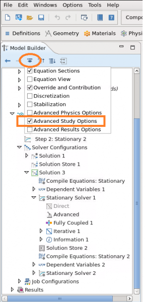
- In the Model Builder, right-click a Study node and select Cluster Computing, as shown in the picture below:
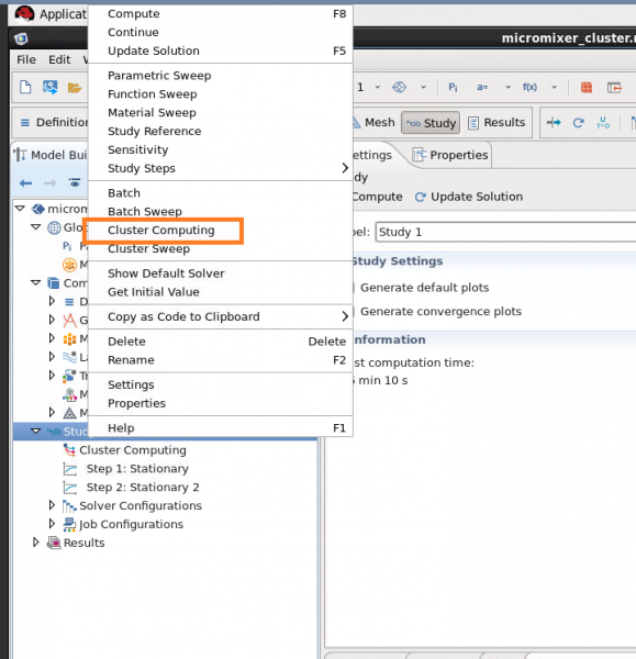
- In the Cluster Computing node's setting window, select General from the Cluster type list. Provide the name of Host file as hostfile. Browse to the directory where your COMSOL input file is located, as shown in the picture below:
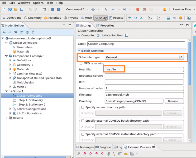
- Save all the settings. Then you should be able to run an interactive parallel COMSOL job at OSC
Supercomputer:
Fields of Science:
CP2K
CP2K is a quantum chemistry and solid state physics software package that can perform atomistic simulations of solid state, liquid, molecular, periodic, material, crystal, and biological systems. CP2K provides a general framework for different modeling methods such as DFT using the mixed Gaussian and plane waves approaches GPW and GAPW. Supported theory levels include DFTB, LDA, GGA, MP2, RPA, semi-empirical methods and classical force fields. CP2K can do simulations of molecular dynamics, metadynamics, Monte Carlo, Ehrenfest dynamics, vibrational analysis, core level spectroscopy, energy minimization, and transition state optimization using NEB or dimer method.
Availability and Restrictions
Versions
CP2K is available on the OSC clusters. These are the versions currently available:
| VERSION | Owens | Pitzer | Notes |
|---|---|---|---|
| 6.1* | X | X | (owens) gnu/7.3.0 intelmpi/2018.3 (pitzer) gnu/4.8.5 openmpi/3.1.6-hpcx (pitzer) gnu/7.3.0 intelmpi/2018.3 (pitzer) gnu/7.3.0 openmpi/3.1.4-hpcx |
| 7.1 | X | X | gnu/8.4.0 intelmpi/2019.7 |
| 2022.2 | X | gnu/11.2.0 openmpi/4.1.4-hpcx |
* See known issues
You can use module spider cp2k to view available modules for a given machine. Feel free to contact OSC Help if you need other versions for your work.
Access
CP2K is available to all OSC users.
Publisher/Vendor/Repository and License Type
CP2K, GNU General Public License
Usage
IMPORTANT NOTE: You need to load the prerequisite compiler and MPI modules before you can load CP2K. To determine those modules, use
module spider cp2k/{version}.We have found some types of CP2K jobs would fail or crash nodes using cp2k.popt and cp2k.psmp from MVAPICH2 and OpenMPI builds due to unstable numerical issues. It is recommended to use Intel MPI, which is more stable unless you experience any other issue.
Usage
Set-up
CP2K usage is controlled via modules. Load one of the CP2K modulefiles at the command line, in your shell initialization script, or in your batch scripts. You need to load the prerequisite compiler and MPI modules before you can load CP2K. To determine those modules, use module spider cp2k/7.1.
Batch Usage
When you log into pitzer.osc.edu you are actually logged into the login node. To gain access to the vast resources in the computing environment, you must submit your job to the batch system for execution. Batch jobs can request mutiple nodes/cores and compute time up to the limits of the OSC systems. Refer to Queues and Reservations and Batch Limit Rules for more info. Batch jobs run on the compute nodes of the system and not on the login node. It is desirable for big problems since more resources can be used.
Interactive Batch Session
For an interactive batch session one can run the following command:
sinteractive -A <project-account> -n 1 -t 00:20:00
which requests one core (-n 1), for a walltime of 20 minutes (-t 00:20:00). You may adjust the numbers per your need.
Non-interactive Batch Job
A batch script can be created and submitted for a serial or parallel run. You can create the batch script using any text editor you like in a working directory on the system of your choice. Below is the example batch script for a parallel run:
#!/bin/bash #SBATCH --nodes=2 #SBATCH --time=1:00:0 #SBATCH --account=<project-account> #SBATCH --gres=pfsdir module load gnu/8.4.0 intelmpi/2019.7 module load cp2k/7.1 module list cp job.inp $PFSDIR/job.inp cd $PFSDIR srun cp2k.popt -i job.inp -o job.out.$SLURM_JOB_ID cp job.out.$SLURM_JOB_ID $SLURM_SUBMIT_DIR/job.out.$SLURM_JOB_ID
This script uses the Scratch storage system, which is designed to synchronize storage across nodes temporarily, more information is available under the storage documentation in the "Further reading" section.
Known Issues
Update: 06/10/2021
Version: 6.1
Version: 6.1
CP2K 6.1 Floating-point exception on Pitzer Cascade Lakes (48-core) node:
Program received signal SIGFPE: Floating-point exception - erroneous arithmetic operation. Backtrace for this error:
Thid could be a bug in libxsmm 1.9.0 which is released on Mar 15, 2018 (Cascade Lake is launched in 2019). The bug has been fixed in cp2k/7.1.
Further Reading
General documentation is available from the CP2K website.
Scratch Storage documentation is available from the Storage Guide
Service:
Fields of Science:
CUDA
CUDA™ (Compute Unified Device Architecture) is a parallel computing platform and programming model developed by Nvidia that enables dramatic increases in computing performance by harnessing the power of the graphics processing unit (GPU).
Availability and Restrictions
Versions
CUDA is available on the clusters supporting GPUs. The versions currently available at OSC are:
| Version | Owens | Pitzer | Ascend | cuDNN library |
|---|---|---|---|---|
| 8.0.44 | X | 5.1.5 | ||
| 8.0.61 | X | 6.0.21 | ||
| 9.0.176 | X | X | 7.3.0 | |
| 9.1.85 | X | X | 6.0.21 and 7.0.5 | |
| 9.2.88 | X | X | 7.1.4 | |
| 10.0.130 | X | X | 7.2.4 | |
| 10.1.168 | X | X | 7.6.5 | |
| 10.2.89 | X* | X* | 7.6.5 | |
| 11.0.3 | X | X | X | 8.0.5 |
| 11.1.1 | X | X | 8.0.5 | |
| 11.2.2 | X | X | 8.1.1 | |
| 11.5.2 | X | X | 8.3.2 | |
| 11.6.1 | X | X | X | 8.3.2 |
| 11.6.2 | X | |||
| 11.7.1 | X* | |||
| 11.8.0 | X | X | X | 8.8.1 |
* Current default version
From CUDA 11 onwards, applications compiled with a CUDA major release can have minor version compatibility, meaning you may run a CUDA 11 application with any CUDA 11.x toolkit. See https://docs.nvidia.com/deploy/cuda-compatibility/#minor-version-compati... for more detail.
You can use module spider cuda to view available modules for a given machine. Feel free to contact OSC Help if you need other versions for your work.
Access
CUDA is available for use by all OSC users.
Publisher/Vendor/Repository and License Type
Nvidia, Freeware
Usage
Usage on Owens
Set-up on Owens
To load the default version of CUDA module, usemodule load cuda. To select a particular software version, use module load cuda/version.
GPU Computing SDK
The NVIDIA GPU Computing SDK provides hundreds of code samples and covers a wide range of applications/techniques to help you get started on the path of writing software with CUDA C/C++ or DirectCompute.
Programming in CUDA
Please visit the following link to learn programming in CUDA, http://developer.nvidia.com/cuda-education-training. The link also contains tutorials on optimizing CUDA codes to obtain greater speedups.
Compiling CUDA Code
Many of the tools loaded with the CUDA module can be used regardless of the compiler modules loaded. However, CUDA codes are compiled with nvcc, which depends on the GNU compilers. In particular, if you are trying to compile CUDA codes and encounter a compiler error such as
#error -- unsupported GNU version! gcc versions later than X are not supported!
then you need to load an older GNU compiler with the module load gnu/version command (if compiling standard C code with GNU compilers) or the module load gcc-compatibility/version command (if compiling standard C code with Intel or PGI compilers).
One can type module show cuda-version-number to view the list of environment variables.
To compile a cuda code contained in a file, let say mycudaApp.cu, the following could be done after loading the appropriate CUDA module: nvcc -o mycudaApp mycudaApp.cu. This will create an executable by name mycudaApp.
The environment variable OSC_CUDA_ARCH defined in the module can be used to specify the CUDA_ARCH, to compile with nvcc -o mycudaApp -arch=$OSC_CUDA_ARCH mycudaApp.cu.
Important: The devices are configured in exclusive mode. This means that 'cudaSetDevice' should NOT be used if requesting one GPU resource. Once the first call to CUDA is executed, the system will figure out which device it is using. If both cards per node is in use by a single application, please use 'cudaSetDevice'.
Debugging CUDA code
cuda-gdb can be used to debug CUDA codes. module load cuda will make it available to you. For more information on how to use the CUDA-GDB please visit http://developer.nvidia.com/cuda-gdb.
Detecting memory access errors
CUDA-MEMCHECK could be used for detecting the source and cause of memory access errors in your program. For more information on how to use CUDA-MEMCHECK please visit http://developer.nvidia.com/cuda-memcheck.
Setting the GPU compute mode on Owens
The GPUs on Owens can be set to different compute modes as listed here.
The default compute mode is the default setting on our GPU nodes (--gpu_cmode=shared), so you don't need to specify if you require this mode. With this mode, mulitple CUDA processes across GPU nodes are allowed, e.g CUDA processes via MPI. So, if you need to run a MPI-CUDA job, just keep the default compute mode. Should you need to use another compute mode, use --gpu_cmode to specify the mode setting. For example:
--nodes=1 --ntasks-per-node=28 --gpus-per-node=1 --gpu_cmode=exclusive
Batch Usage on Owens
When you log into owens.osc.edu you are actually logged into a linux box referred to as the login node. To gain access to the mutiple processors in the computing environment, you must submit your job to the batch system for execution. Batch jobs can request mutiple nodes/cores and compute time up to the limits of the OSC systems. Refer to Queues and Reservations and Batch Limit Rules for more info.
Interactive Batch Session
For an interactive batch session one can run the following command:
sinteractive -A <project-account> -N 1 -n 28 -g 1 -t 00:20:00
which requests one whole node with 28 cores (-N 1 -n 1), for a walltime of 20 minutes (-t 00:20:00), with one gpu (-g 1). You may adjust the numbers per your need.
Non-interactive Batch Job (Serial Run)
A batch script can be created and submitted for a serial or parallel run. You can create the batch script using any text editor you like in a working directory on the system of your choice. Below is the example batch script (job.txt) for a serial run:
#!/bin/bash #SBATCH -- time=01:00:00 #SBATCH --nodes=1 --ntasks-per-node=1:gpus=1 #SBATCH --job-name compute #SBATCH --account=<project-account> module load cuda cd $HOME/cuda cp mycudaApp $TMPDIR cd $TMPDIR ./mycudaApp
Usage on Pitzer
Set-up on Pitzer
To load the default version of CUDA module, usemodule load cuda.
GPU Computing SDK
The NVIDIA GPU Computing SDK provides hundreds of code samples and covers a wide range of applications/techniques to help you get started on the path of writing software with CUDA C/C++ or DirectCompute.
Programming in CUDA
Please visit the following link to learn programming in CUDA, http://developer.nvidia.com/cuda-education-training. The link also contains tutorials on optimizing CUDA codes to obtain greater speedups.
Compiling CUDA Code
Many of the tools loaded with the CUDA module can be used regardless of the compiler modules loaded. However, CUDA codes are compiled with nvcc, which depends on the GNU compilers. In particular, if you are trying to compile CUDA codes and encounter a compiler error such as
#error -- unsupported GNU version! gcc versions later than X are not supported!
then you need to load an older GNU compiler with the module load gnu/version command (if compiling standard C code with GNU compilers) or the module load gcc-compatibility/version command (if compiling standard C code with Intel or PGI compilers).
One can type module show cuda-version-number to view the list of environment variables.
To compile a cuda code contained in a file, let say mycudaApp.cu, the following could be done after loading the appropriate CUDA module: nvcc -o mycudaApp mycudaApp.cu. This will create an executable by name mycudaApp.
The environment variable OSC_CUDA_ARCH defined in the module can be used to specify the CUDA_ARCH, to compile with nvcc -o mycudaApp -arch=$OSC_CUDA_ARCH mycudaApp.cu.
Important: The devices are configured in exclusive mode. This means that 'cudaSetDevice' should NOT be used if requesting one GPU resource. Once the first call to CUDA is executed, the system will figure out which device it is using. If both cards per node is in use by a single application, please use 'cudaSetDevice'.
Debugging CUDA code
cuda-gdb can be used to debug CUDA codes. module load cuda will make it available to you. For more information on how to use the CUDA-GDB please visit http://developer.nvidia.com/cuda-gdb.
Detecting memory access errors
CUDA-MEMCHECK could be used for detecting the source and cause of memory access errors in your program. For more information on how to use CUDA-MEMCHECK please visit http://developer.nvidia.com/cuda-memcheck.
Setting the GPU compute mode on Pitzer
The GPUs on Pitzer can be set to different compute modes as listed here.
The default compute mode is the default setting on our GPU nodes (--gpu_cmode=shared), so you don't need to specify if you require this mode. With this mode, mulitple CUDA processes across GPU nodes are allowed, e.g CUDA processes via MPI. So, if you need to run a MPI-CUDA job, just keep the default compute mode. Should you need to use another compute mode, use --gpu_cmode to specify the mode setting. For example:
--nodes=1 --ntasks-per-node=40 --gpus-per-node=1 --gpu_cmode=exclusive
Batch Usage on Pitzer
When you log into pitzer.osc.edu you are actually logged into a linux box referred to as the login node. To gain access to the mutiple processors in the computing environment, you must submit your job to the batch system for execution. Batch jobs can request mutiple nodes/cores and compute time up to the limits of the OSC systems. Refer to Queues and Reservations and Batch Limit Rules for more info.
Interactive Batch Session
For an interactive batch session one can run the following command:
sinteractive -A <project-account> -N 1 -n 40 -g 2 -t 00:20:00
which requests one whole node (-N 1), 40 cores (-n 40), 2 gpus (-g 2), and a walltime of 20 minutes (-t 00:20:00). You may adjust the numbers per your need.
Non-interactive Batch Job (Serial Run)
A batch script can be created and submitted for a serial or parallel run. You can create the batch script using any text editor you like in a working directory on the system of your choice. Below is the example batch script (job.txt) for a serial run:
#!/bin/bash #SBATCH --time=01:00:00 #SBATCH --nodes=1 --ntasks-per-node=1 --gpus-per-node=1 #SBATCH --job-name Compute #SBATCH --account=<project-account> module load cuda cd $HOME/cuda cp mycudaApp $TMPDIR cd $TMPDIR ./mycudaApp
GNU Compiler Support for NVCC
| CUDA Version | Max supported GCC version |
|---|---|
| 9.2.88 - 10.0.130 | 7 |
| 10.1.168 - 10.2.89 | 8 |
| 11.0 | 9 |
| 11.1 - 11.4.0 | 10 |
| 11.4.1 - 11.8 | 11 |
| 12.0 | 12.1 |
Further Reading
Online documentation is available on the CUDA homepage.
Compiler support for the latest version of CUDA is available here.
CUDA optimization techniques.
Service:
Technologies:
Fields of Science:
Caffe
Caffe is "
From their README:
Caffe is a deep learning framework made with expression, speed, and modularity in mind. It is developed by the Berkeley Vision and Learning Center (BVLC) and by community contributors. Yangqing Jia created the project during his PhD at UC Berkeley. Caffe is released under the BSD 2-Clause license.
Caffe also includes interfaces for both Python and Matlab, which have been built but have not been tested.
Availability and Restrictions
Versions
The following versions of Caffe are available on OSC clusters:
| Version | Owens |
|---|---|
| 1.0.0-rc3 | X* |
* Current Default Version
You can use module spider caffe to view available modules for a given machine. Feel free to contact OSC Help if you need other versions for your work.
The current version of Caffe on Owens requires cuda/8.0.44 for GPU calculations.
Access
Caffe is available to all OSC users. If you have any questions, please contact OSC Help.
Publisher/Vendor/Repository and License Type
Berkeley AI Research, Open source
Usage
Usage on Owens
Setup on Owens
To configure the Owens cluster for the use of Caffe, use the following commands:
module load caffe
Batch Usage on Owens
Batch jobs can request mutiple nodes/cores and compute time up to the limits of the OSC systems. Refer to Queues and Reservations for Owens, and Scheduling Policies and Limits for more info. In particular, Caffe should be run on a GPU-enabled compute node.
An Example of Using Caffe with MNIST Training Data on Owens
Below is an example batch script (job.txt) for using Caffe, see this resource for a detailed explanation http://caffe.berkeleyvision.org/gathered/examples/mnist.html
#!/bin/bash
#SBATCH --job-name=Caffe
#SBATCH --nodes=1 --ntask-per-node=28:gpu
#SBATCH --time=30:00
#SBATCH --account <project-account>
. /etc/profile.d/lmod.sh
# Load the modules for Caffe
ml caffe
# Migrate to job temp directory and copy folders over
cd $TMPDIR
cp -r $CAFFE_HOME/{examples,data} .
# Download, create, train
./data/mnist/get_mnist.sh
./examples/mnist/create_mnist.sh
./examples/mnist/train_lenet.sh
# Serialize log files
echo; echo 'LOG 1'
cat convert_mnist_data.bin.$(hostname)*
echo; echo 'LOG 2'
cat caffe.INFO
echo; echo 'LOG 3'
cat convert_mnist_data.bin.INFO
echo; echo 'LOG 4'
cat caffe.$(hostname).*
cp examples/mnist/lenet_iter_10000.* $SLURM_SUBMIT_DIR
In order to run it via the batch system, submit the job.txt file with the following command:
sbatch job.txt
Further Reading
Supercomputer:
Service:
Technologies:
Fields of Science:
Cell Ranger
Cell Ranger is a cell analysis library for generate feature-barcode matrices, perform Analysis for RNA samples. Cell Ranger works in pipelines for it's RNA sequencing analysis which allows it to: process raw sequencing output, read alignment, generate gene-cell matrices, and can perform downstream analyses such as clustering and gene expression analysis.
Availability and Restrictions
Versions
Cell Ranger is available on the Pitzer Cluster. The versions currently available at OSC are:
| Version | Pitzer | Notes |
|---|---|---|
| 7.0.0 | X* | |
| 7.2.0 | X |
* Current Default Version
You can use module spider cellranger to view available modules for a given machine. Feel free to contact OSC Help if you need other versions for your work.
Access
Cell Ranger is available to only academic OSC users. Please review the license agreement and 10x Privacy Policy before use. If you have any questions, please contact OSC Help.
Publisher/Vendor/Repository and License Type
The 10x Genomics group, Closed source (academic)
Usage
Usage on Pitzer
Set-up
To configure your environment for use of Cell Ranger, run the following command: module load cellranger. The default version will be loaded. To select a particular Cell Ranger version, use module load cellranger/version. For example, use module load cellranger/7.0.0 to load Cell Ranger 7.0.0.
Further Reading
Tag:
Supercomputer:
Service:
Fields of Science:
Clara Parabricks
Clara Parabricks is a powerful toolkit designed for genomic analysis. It is primarily designed for GPU computation.
Availability and Restrictions
Versions
Clara Parabricks is available on Pitzer and Owens Clusters. The versions currently available at OSC are the following:
| Version | Owens | Pitzer | Notes |
|---|---|---|---|
| 4.0.0-1 | X* | X* |
* Current default version
You can use module spider clara-parabricks to view available modules for a given machine. Feel free to contact OSC Help if you need other versions for your work.
Access
Clara-Parabricks is available to all OSC users. If you have any questions, please contact OSC Help.
Publisher/Vendor/Repository and License Type
Open source
Usage
Usage on Owens
Set-up
To load the module for the default version of Parabricks, which initializes your environment for the Clara-Parabricks application, use
module load clara-parabricks. To select a particular software version, use module load clara-parabricks/version. For example, use module load clara-parabricks/4.0.0-1 to load Parabricks version 4.0.0-1; and use module help clara-parabricks/4.0.0-1 to view details, such as compiler prerequisites, additional modules required for specific executables, the suffixes of executables, etc.; some versions require specific prerequisite modules, and such details may be obtained with the command module spider clara-parabricks/version.Batch Usage
When you log into Owens you are actually connected to a login node. To access the compute nodes, you must submit a job to the batch system for execution. Batch jobs can request multiple nodes/cores and compute time up to the limits of the OSC systems. Refer to Queues and Reservations and Batch Limit Rules for more info.
Interactive Batch Session
For an interactive batch session, one can run the following command:sinteractive -A <project-account> -N 1 -n 28 -t 1:00:00which gives you one node with 28 cores (
-N 1 -n 28), with 1 hour (-t 1:00:00). You may adjust the numbers per your need.Usage on Pitzer
Set-up
To load the module for the default version of Parabricks, which initializes your environment for the Clara-Parabricks application, use
module load clara-parabricks. To select a particular software version, use module load clara-parabricks/version. For example, use module load clara-parabricks/4.0.0-1 to load Parabricks version 4.0.0-1; and use module help clara-parabricks/4.0.0-1 to view details, such as, compiler prerequisites, additional modules required for specific executables, the suffixes of executables, etc.; some versions require specific prerequisite modules, and such details may be obtained with the command module spider clara-parabricks/version.Batch Usage
When you log into Owens you are actually connected to a login node. To access the compute nodes, you must submit a job to the batch system for execution. Batch jobs can request multiple nodes/cores and compute time up to the limits of the OSC systems. Refer to Queues and Reservations and Batch Limit Rules for more info.
Interactive Batch Session
For an interactive batch session, one can run the following command:sinteractive -A <project-account> -N 1 -n 28 -t 1:00:00which gives you one node with 28 cores (
-N 1 -n 28), with 1 hour (-t 1:00:00). You may adjust the numbers per your need.Further Reading
Service:
Technologies:
Fields of Science:
Clustal W
Clustal W is a multiple sequence alignment program written in C++.
Availability and Restrictions
Versions
The following versions of bedtools are available on OSC clusters:
| Version | Owens | Pitzer |
|---|---|---|
| 2.1 | X* | X* |
* Current default version
You can use module spider clustalw to view available modules for a given machine. Feel free to contact OSC Help if you need other versions for your work.
Access
Clustal W is available to all OSC users. If you have any questions, please contact OSC Help.
Publisher/Vendor/Repository and License Type
GNU Lesser GPL.
Usage
Usage on Owens
Set-up
To configure your environment for use of metilene, run the following command:
module load clustalw. The default version will be loaded. To select a particular MUSCLE version, use module load clustalw/version. For example, use module load clustalw/2.1 to load Clustal W 2.1.Usage on Pitzer
Set-up
To configure your environment for use of metilene, run the following command:
module load clustalw. The default version will be loaded. To select a particular MUSCLE version, use module load clustalw/version. For example, use module load clustalw/2.1 to load Clustal W 2.1.Further Reading
Service:
Fields of Science:
Connectome
Connectome is an open-source visualization and discovery tool used to explore data generated by the Human Connectome Project. The distribution includes wb_view, a GUI-based visualization platform, and wb_command, a command-line program for performing a variety of algorithmic tasks using volume, surface, and grayordinate data.
Availability and Restrictions
Versions
The following versions are available on OSC clusters:
| Version | Pitzer |
|---|---|
| 1.5.0 | X* |
* Current default version
You can use module spider connectome to view available modules for a given machine. Feel free to contact OSC Help if you need other versions for your work.
Access
Connectome is available to all OSC users. If you have any questions, please contact OSC Help.
Publisher/Vendor/Repository and License Type
Connectome Workbench is made available via the GNU General Public License, version 2. The full license is available from here.
Usage
Usage on Pitzer
Set-up
To configure your environment for use of connectome, run the following command: module load connectome. The default version will be loaded. To select a particular connectome version, use module load connectome/version. For example, use module load connectome/1.5.0 to load Connectome 1.5.0.
If you want the hardware-accelerated 3D graphics, use these on a compute node with a GPU:
module load virutalgl/2.6.5 module load connectome viglrun wb_view
The command will open the GUI environment, thus we recommend Ondemand VDI or Desktop.
Further Reading
Supercomputer:
Service:
Fields of Science:
Connectome Workbench
Connectome Workbench is an open source, freely available visualization and analysis tool for neuroimaging data, especially data generated by the Human Connectome Project.
Availability and Restrictions
Versions
Connectome Workbench is available on Owens and Pitzer clusters. These are the versions currently available:
| Version | Owens | Pitzer | Notes |
|---|---|---|---|
| 1.3.2 | X* | X* | |
| 1.5.0 | X | X |
* Current default version
You can use module spider connectome-workbench to view available modules for a given machine. Feel free to contact OSC Help if you need other versions for your work.
Access
Connectome Workbench is available to all OSC users.
Publisher/Vendor/Repository and License Type
Washington University School of Medicine, GPL
Usage
Set-up
To configure your environment for use of the workbench, run the following command: module load connectome-workbench virtualgl. The default version will be loaded; the virtualgl module is required as well on some platforms. To select a particular version, use module load connectome-workbench/version. For example, use module load connectome-workbench/1.3.2 to load Connectome Workbench 1.3.2.
Further Reading
General documentation is available from the Connectome Workbench hompage.
Service:
Fields of Science:
Cufflinks
Cufflinks is a program that analyzes RNA -Seq samples. It assembles aligned RNA-Seq reads into a set of transcripts, then inspects the transcripts to estimate abundances and test for differential expression and regulation in the RNA-Seq reads.
Availability and Restrictions
Versions
Cufflinks is available on the Owens Cluster. The versions currently available at OSC are:
| Version | Owens |
|---|---|
| 2.2.1 | X* |
* Current Default Version
You can use module spider cufflinks to view available modules for a given machine. Feel free to contact OSC Help if you need other versions for your work.
Access
Cufflinks is available to all OSC users. If you have any questions, please contact OSC Help.
Publisher/Vendor/Repository and License Type
Cole Trapnell et al., Open source
Usage
Usage on Owens
Set-up
To configure your enviorment for use of Cufflinks, use command module load cufflinks. This will load the default version.
Further Reading
Supercomputer:
Fields of Science:
DS9
SAOImageDS9 is a astronomical imaging and data visualization application. DS9 provides support for FITS images, binary tables, multiple frame buffers, region manipulation, and colormaps display options
Availability and Restrictions
The following versions of DS9 are available on OSC clusters:
| Version | Owens | Pitzer |
|---|---|---|
| 7.8.3 | X* | X* |
* Current default version
You can use module spider ds9to view available modules for a given machine. Feel free to contact OSC Help if you need other versions for your work.
Access
DS9 is available to all OSC users. If you have any questions, please contact OSC Help.
Publisher/Vendor/Repository and License Type
Jessica Mink, Smithsonian Astrophysical Observatory/ Open source
Usage
Usage on Owens
Set-up
To configure your environment for use of DS9, run the following command:
module load ds9. The default version will be loaded. To select a particular DS9 version, use module load ds9/version . For example, use module load ds9/7.8.3to load DS9 7.8.3.Usage on Pitzer
Set-up
To configure your environment for use of DS9, run the following command:
module load ds9. The default version will be loaded. To select a particular DS9 version, use module load ds9/version . For example, use module load ds9/7.8.3to load DS9 7.8.3.Further Reading
Tag:
Service:
Fields of Science:
DSI Studio
DSI Studio is a tractography software tool that maps brain connections and correlates findings with neuropsychological disorders. It is a collective implementation of several diffusion MRI methods, including diffusion tensor imaging (DTI), generalized q-sampling imaging (GQI), q-space diffeomorphic reconstruction (QSDR), diffusion MRI connectometry, and generalized deterministic fiber tracking.
Availability and Restrictions
The following versions of DSI Studio are available on OSC clusters:
| Version | Pitzer |
|---|---|
| 2.0 | X |
* Current default version
You can use module spider dsi-studio to view available modules for a given machine. Feel free to contact OSC Help if you need other versions for your work.
Access
DSI Studio is available to all OSC users. If you have any questions, please contact OSC Help.
Publisher/Vendor/Repository and License Type
DSI Studio is free and licensing information for both academic and non-academic licenses is available at the DSI Studio homepage.
Please refer to the citation page about how to acknowledge DSI Studio.
Usage
Usage on Pitzer
Set-up
To configure your environment for use of DSI Studio, run the following command:
module load dsi-studio. The default version will be loaded. To select a particular version, use module load dsi-studio/version. For example, use module load dsi-studio/2021.May to load DSI Studio 2.0. It is also recommended you use in conjunction with module load singularity.DSI Studio is installed in a singularity container. DSI_IMG environment variable contains the container image file path. So, an example usage would be
module load dsi-studio singularity exec $DSI_IMG dsi_studio
This command will open the DSI Studio GUI environment, and we recommend Ondemand VDI or Desktop for GUI.
For more information about singularity usages, please read OSC singularity page
Further Reading
Supercomputer:
Service:
Fields of Science:
Darshan
Darshan is a lightweight "scalable HPC I/O characterization tool
Availability and Restrictions
Versions
The following versions of Darshan are available on OSC clusters:
| Version | Owens | Pitzer |
|---|---|---|
| 3.1.2 | X | |
| 3.1.4 | X | |
| 3.1.5-pre1 | X | |
| 3.1.5 | X | |
| 3.1.6 | X | X |
| 3.1.8 | X* | X* |
| 3.2.1 | X | X |
* Current default version
You can use module spider darshan to view available modules for a given machine. Feel free to contact OSC Help if you need other versions for your work.
Access
Darshan is available to all OSC users. If you have any questions, please contact OSC Help.
Publisher/Vendor/Repository and License Type
MCSD, Argonne National Laboratory, Open source
Usage
Usage on Owens & Pitzer
Setup
To configure the Owens/Pitzer cluster for Darshan run module spider darshan/VERSION to find supported compiler and MPI implementations, e.g.
$ module spider darshan/3.2.1 ------------------------------------------------------------------------------------------------ darshan: darshan/3.2.1 ------------------------------------------------------------------------------------------------ You will need to load all module(s) on any one of the lines below before the "darshan/3.2.1" module is available to load. intel/19.0.3 intelmpi/2019.7 intel/19.0.3 mvapich2/2.3.1 intel/19.0.3 mvapich2/2.3.2 intel/19.0.3 mvapich2/2.3.3 intel/19.0.3 mvapich2/2.3.4 intel/19.0.3 mvapich2/2.3.5 intel/19.0.5 intelmpi/2019.3 intel/19.0.5 intelmpi/2019.7 intel/19.0.5 mvapich2/2.3.1 intel/19.0.5 mvapich2/2.3.2 intel/19.0.5 mvapich2/2.3.3 intel/19.0.5 mvapich2/2.3.4 intel/19.0.5 mvapich2/2.3.5
then switch to the favorite programming environment and load the Darshan module:
$ module load intel/19.0.5 mvapich2/2.3.5 $ module load darshan/3.2.1
Batch Usage
Batch jobs can request mutiple nodes/cores and compute time up to the limits of the OSC systems. Refer to Queues and Reservations (Owens, Pitzer) and Scheduling Policies and Limits for more info.
If you have an MPI-based program the syntax is as simple as
module load darshan # basic call to darshan export MV2_USE_SHARED_MEM=0 export LD_PRELOAD=$OSC_DARSHAN_DIR/lib/libdarshan.so srun [args] ./my_mpi_program # to show evidence that Darshan is working and to see internal timing export DARSHAN_INTERNAL_TIMING=yes srun [args] ./my_mpi_program
An Example of Using Darshan with MPI-IO
Below is an example batch script (darshan_mpi_pfsdir_test.sh) for testing MPI-IO and POSIX-IO. Because the files generated here are large scratch files there is no need to retain them.
#!/bin/bash
#SBATCH --job-name="darshan_mpi_pfsdir_test"
#SBATCH --ntasks=4
#SBATCH --ntasks-per-node=2
#SBATCH --output=rfm_darshan_mpi_pfsdir_test.out
#SBATCH --time=0:10:0
#SBATCH -p parallel
#SBATCH --gres=pfsdir:ess
# Setup Darshan
module load intel
module load mvapich2
module load darshan
export DARSHAN_LOGFILE=${LMOD_SYSTEM_NAME}_${SLURM_JOB_ID/.*/}_${SLURM_JOB_NAME}.log
export DARSHAN_INTERNAL_TIMING=yes
export MV2_USE_SHARED_MEM=0
export LD_PRELOAD=$OSC_DARSHAN_DIR/lib/libdarshan.so
# Prepare the scratch files and run the cases
cp ~support/share/reframe/source/darshan/io-sample.c .
mpicc -o io-sample io-sample.c -lm
for x in 0 1 2 3; do dd if=/dev/zero of=$PFSDIR/read_only.$x bs=2097152000 count=1; done
shopt -s expand_aliases
srun ./io-sample -p $PFSDIR -b 524288000 -v
# Generat report
darshan-job-summary.pl --summary $DARSHAN_LOGFILE
In order to run it via the batch system, submit the darshan_mpi_pfsdir_test.sh file with the following command:
sbatch darshan_mpi_pfsdir_test.sh
Further Reading
Service:
Technologies:
Fields of Science:
Desmond
Desmond is a software package that perform high-speed molecular dynamics simulations of biological systems on conventional commodity clusters, general-purpose supercomputers, and GPUs. The code uses novel parallel algorithms and numerical techniques to achieve high performance and accuracy on platforms containing a large number of processors, but may also be executed on a single computer. Desmond includes code optimized for machines with an NVIDIA GPU.
Availability and Restrictions
Versions
The Desmond package is available on Owens. The versions currently available at OSC are:
| Version | Owens | Note |
|---|---|---|
| 2018.2 | X | |
| 2019.1 | X* | |
| 2020.1 | X | GPU support only |
| 2022.4 | X | GPU support only |
* Current default version
You can use module spider desmond to view available modules for a given machine. Feel free to contact OSC Help if you need other versions for your work.
Access for Academic Users
Desmond is available to academic OSC users. Please review the license agreement carefully before use. If you have any questions, please contact OSC Help.
Publisher/Vendor/Repository and License Type
D. E. Shaw Research, Non-Commercial
Usage
Usage on Owens
Set-up
To set up your environment for desmond load one of its module files:
module load desmond/2018.2
If you already have input and configuration files ready, here is an example batch script that uses Desmond non-interactively via the batch system:
#!/bin/bash #SBATCH --job-name multisim-batch #SBATCH --time=0:20:00 #SBATCH --nodes=1 #SBATCH --ntasks-per-node=24 #SBATCH --account=<account># Example Desmond single-node batch script. sstat -j $SLURM_JOB_ID export module load desmond/2018.2 module list sbcast -p desmondbutane.msj $TMPDIR/desmondbutane.msj sbcast -p desmondbutane.cfg $TMPDIR/desmondbutane.cfg sbcast -p desmondbutane.cms $TMPDIR/desmondbutane.cms cd $TMPDIR $SCHRODINGER/utilities/multisim -HOST localhost -maxjob 1 -cpu 24 -m desmondbutane.msj -c desmondbutane.cfg desmondbutane.cms -mode umbrella -ATTACHED -WAIT ls -l cd $SLURM_SUBMIT_DIR sgather -r $TMPDIR $SLURM_SUBMIT_DIR
The WAIT option forces the multisim command to wait until all tasks of the command are completed. This is necessary for batch jobs to run effectively. The HOST option specifies how tasks are distributed over processors.
Set-up via Maestro
Desmond comes with the Schrodinger interactive builder, Maestro. To run maestro, connect to OSC OnDemand and luanch a desktop, either via Desktops in the Interactive Apps drop down menu (these were labelled Virtual Desktop Interface (VDI) previously) or via Shell Access in the Clusters drop down menu (these were labelled Interactive HPC Desktop previously). Click "Setup process" below for more detailed instructions. Note that one cannot launch desmond jobs in maestro via the Schrodinger GUI in the Interactive Apps drop down menu.
Setup process
Log in to OSC OnDemand and request a Desktop/VDI session (this first screen shot below does not reflect the current, 2024, labelling in OnDemand).
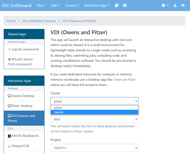
In a Desktop/VDI environment, open a terminal and run (this is a critical step; one cannot launch desmond jobs in maestro via the Schrodinger GUI in the Interactive Apps drop down menu.
module load desmond maestro
In the main window of Maestro, you can open File and import structures or create new project
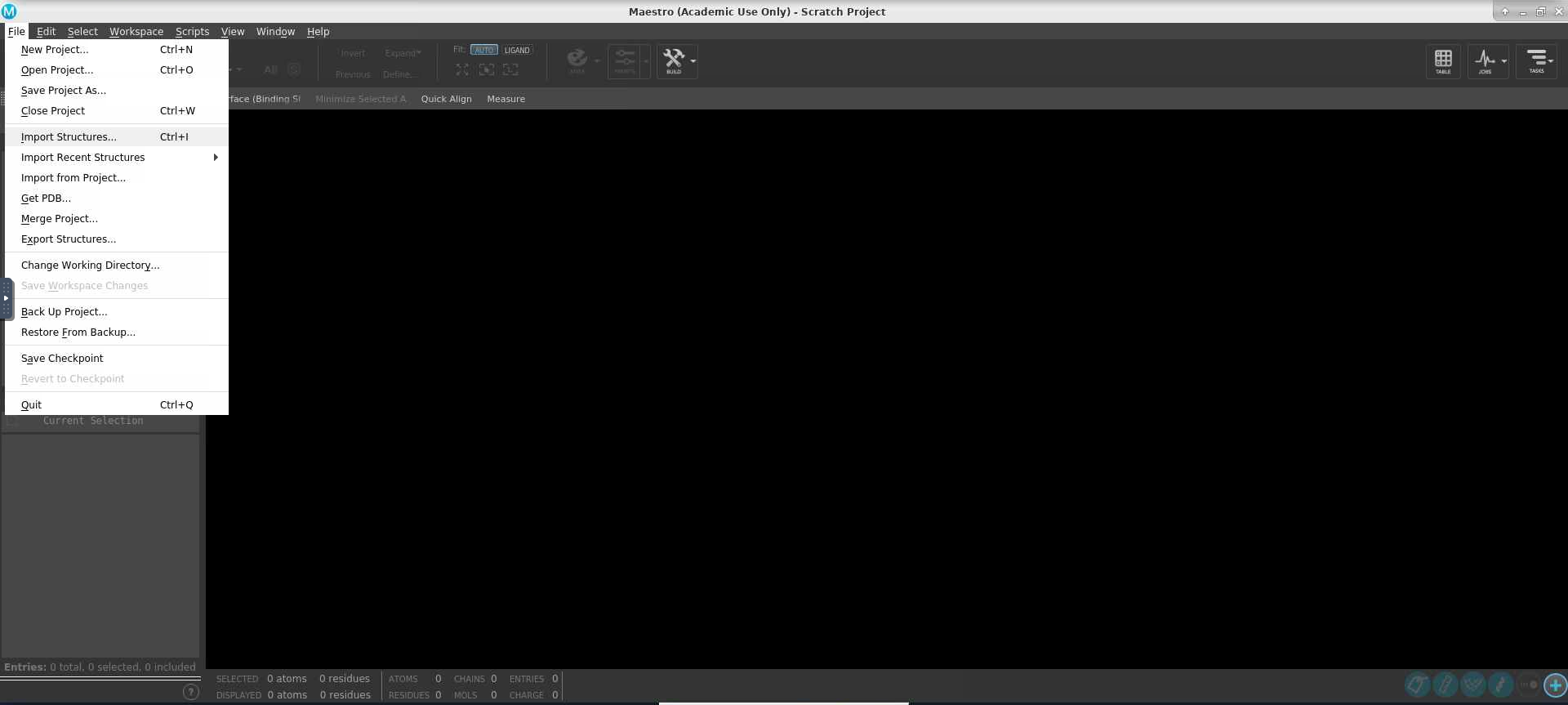
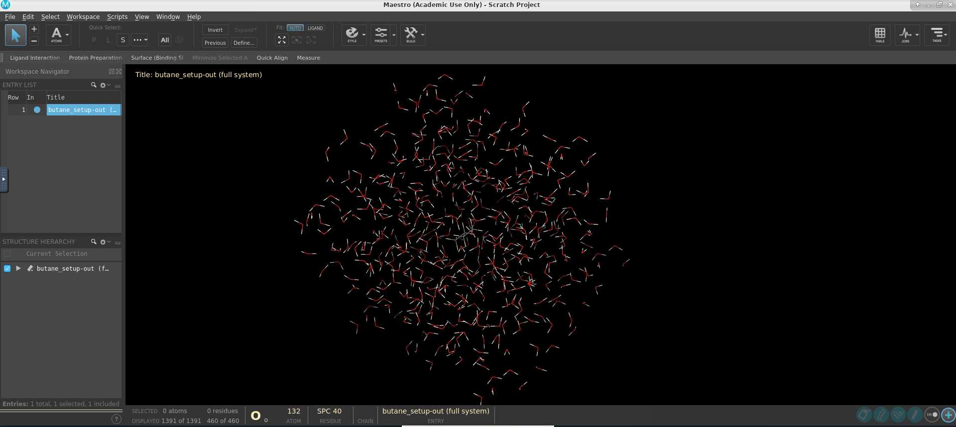
Once the structure is ready, navigate to the top right Tasks icon and find Desmond application; the details of this step depend on the software version; if you do not find desmond listed then use the search bar.
Tasks >> Browse... > Applications tab >> Desmond
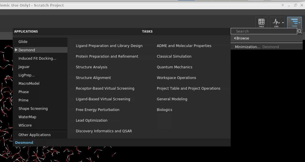
In this example a Minimazation job will be done.
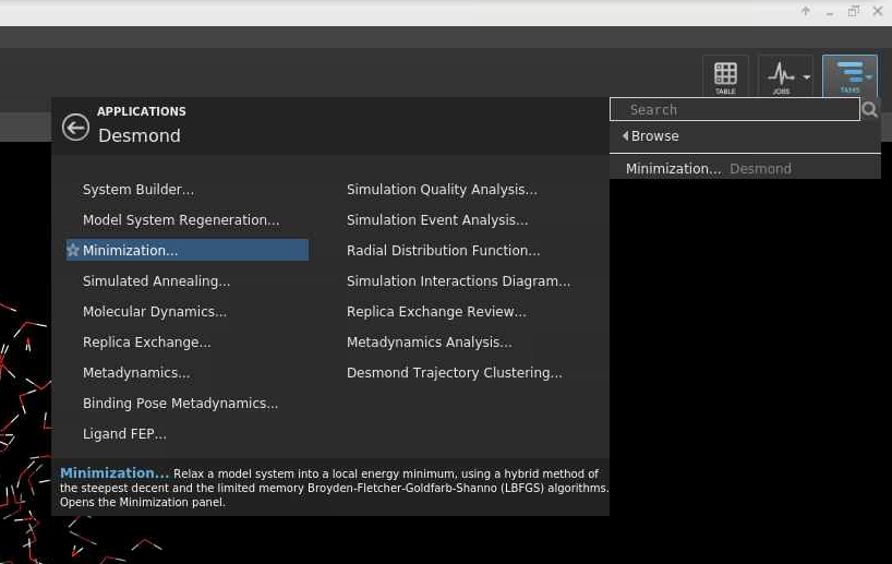
Make sure the Model system is ready:
Model system >> Load from workspace >> Load
You can change the Job name; and you can write out the script and configuration files by clicking Write as shown below:
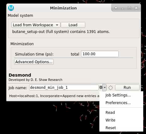
The green text will indicate the job path with the prefix "Job written to...". The path is a new folder located in the working directory indicated earlier.
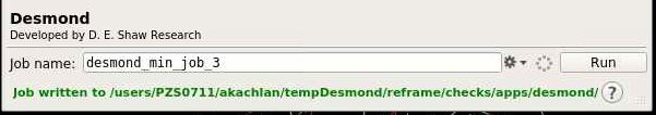
Navigate using the terminal to that directory. You can modify the script to either run the simulation with a GPU or a CPU.
Run simulation with GPU
Navigate using the terminal to that directory and add the required SLURM directives and module commands at the top of the script, e.g.: desmond_min_job_1.sh:
#!/bin/bash #SBATCH --time=0:20:00 #SBATCH --nodes=1 #SBATCH --ntasks-per-node=8 #SBATCH --gpus-per-node=1 #SBATCH --account=<account> module reset module load desmond/2019.1 # Desmond job script starts here
The setup is complete.
Run simulation with CPU only
Navigate using the terminal to that directory and edit the script, e.g.: desmond_min_job_1.sh:
"${SCHRODINGER}/utilities/multisim" -JOBNAME desmond_min_job_1 -HOST localhost -maxjob 1 -cpu 1 -m desmond_min_job_1.msj -c desmond_min_job_1.cfg -description Minimization desmond_min_job_1.cms -mode umbrella -set stage[1].set_family.md.jlaunch_opt=["-gpu"] -o desmond_min_job_1-out.cms -ATTACHED
Delete the -set stage[1].set_family.md.jlaunch_opt=["-gpu"] argument and change the -cpu argument from 1 to the number of CPUs you want, e.g. 8, resulting in
"${SCHRODINGER}/utilities/multisim" -JOBNAME desmond_min_job_1 -HOST localhost -maxjob 1 -cpu 8 -m desmond_min_job_1.msj -c desmond_min_job_1.cfg -description Minimization desmond_min_job_1.cms -mode umbrella -o desmond_min_job_1-out.cms -ATTACHED
Add the required SLURM directives and module commands at the top of the script:
#!/bin/bash #SBATCH --time=0:20:00 #SBATCH --nodes=1 #SBATCH --ntasks-per-node=24 #SBATCH --account=<account> module reset module load desmond/2019.1 # Desmond job script starts here
The setup is complete.
Further Reading
Tag:
Supercomputer:
Service:
Fields of Science:
FASTX-Toolkit
The FASTX-Toolkit is a collection of command line tools for Short-Reads FASTA/FASTQ files preprocessing.
Availability and Restrictions
Verisons
The following versions of FASTX-Toolkit are available on OSC clusters:
| Version | Owens |
|---|---|
| 0.0.14 | X* |
*:Current default version
You can use module spider fastx to view available modules for a given machine. Feel free to contact OSC Help if you need other versions for your work.
Access
FASTX-Toolkit is available to all OSC users. If you have any questions, please contact OSC Help.
Publisher/Vendor/Repository and License Type
Assaf Gordon, Open source
Usage
Usage on Owens
Set-up
To configure your environment for use of FASTX-Toolkit, run the following command:
module load fastx. The default version will be loaded. To select a particular FASTX-Toolkit version, use module load fastx/version. For example, use module load fastx/0.0.14 to load FASTX-Toolkit 0.0.14.Further Reading
Supercomputer:
Service:
Fields of Science:
FFTW
FFTW is a C subroutine library for computing the Discrete Fourier Transform (DFT) in one or more dimensions, of arbitrary input size, and of both real and complex data. It is portable and performs well on a wide variety of platforms.
Availability and Restrictions
Versions
FFTW is available on Ruby, and Owens Clusters. The versions currently available at OSC are:
| Version | Owens | Pitzer | Ascend |
|---|---|---|---|
| 3.3.4 | X | ||
| 3.3.5 | X | ||
| 3.3.8 | X* | X* | |
| 3.3.10 | X | X | X* |
NOTE: FFTW2 and FFTW3 are tracked separately in the module system
You can use module spider fftw2 or module spider fftw3 to view available modules for a given machine. Feel free to contact OSC Help if you need other versions for your work.
Access
FFTW is available to all OSC users. If you have any questions, please contact OSC Help.
Publisher/Vendor/Repository and License Type
www.fftw.org, Open source
Usage
Usage on Owens
Set-up
Initalizing the system for use of the FFTW library is dependent on the system you are using and the compiler you are using. A successful build of your program will depend on an understanding of what module fits your circumstances. To load a particular version, use module load name . For example, use module load fftw3/3.3.4 to load FFTW3 version 3.3.4. You can use module spider fftw to view available modules.
Building with FFTW
The following environment variables are setup when the FFTW library is loaded:
| Variable | Use |
|---|---|
$FFTW3_CFLAGS |
Use during your compilation step for C programs. |
$FFTW3_FFLAGS |
Use during your compilation step for Fortran programs. |
$FFTW3_LIBS |
Use during your link step for the sequential version of the library. |
$FFTW3_LIBS_OMP |
Use during your link step for the OpenMP version of the library. |
$FFTW3_LIBS_MPI |
Use during your link step for the MPI version of the library. |
$FFTW3_LIBS_THREADS |
Use during your link step for the "threads" version of the library. |
below is a set of example commands used to build a file called my-fftw.c .
module load fftw3 icc $FFTW3_CFLAGS my-fftw.c -o my-fftw $FFTW3_LIBS ifort $FFTW3_FFLAGS more-fftw.f -o more-fftw $FFTW3_LIBS
Usage on Pitzer
Set-up
Initalizing the system for use of the FFTW library is dependent on the system you are using and the compiler you are using. A successful build of your program will depend on an understanding of what module fits your circumstances. To load a particular version, use module load fftw3/.
Building with FFTW
The following environment variables are setup when the FFTW library is loaded:
| VARIABLE | USE |
|---|---|
$FFTW3_CFLAGS |
Use during your compilation step for C programs. |
$FFTW3_FFLAGS |
Use during your compilation step for Fortran programs. |
$FFTW3_LIBS |
Use during your link step for the sequential version of the library. |
$FFTW3_LIBS_OMP |
Use during your link step for the OpenMP version of the library. |
$FFTW3_LIBS_MPI |
Use during your link step for the MPI version of the library. |
below is a set of example commands used to build a file called my-fftw.c .
module load fftw3 icc $FFTW3_CFLAGS my-fftw.c -o my-fftw $FFTW3_LIBS ifort $FFTW3_FFLAGS more-fftw.f -o more-fftw $FFTW3_LIBS
Usage on Ascend
Set-up
Initalizing the system for use of the FFTW library is dependent on the system you are using and the compiler you are using. A successful build of your program will depend on an understanding of what module fits your circumstances. To load a particular version, use module spider fftw3 to check what other modules need to be loaded first. Use module load [module name and version] to load the necessary modules. Then use module load fftw3 to load the default FFTW module version.
Building with FFTW
The following environment variables are setup when the FFTW library is loaded:
| VARIABLE | USE |
|---|---|
$FFTW3_CFLAGS |
Use during your compilation step for C programs. |
$FFTW3_FFLAGS |
Use during your compilation step for Fortran programs. |
$FFTW3_LIBS |
Use during your link step for the sequential version of the library. |
$FFTW3_LIBS_OMP |
Use during your link step for the OpenMP version of the library. |
$FFTW3_LIBS_MPI |
Use during your link step for the MPI version of the library. |
below is a set of example commands used to build a file called my-fftw.c .
module load fftw3 icc $FFTW3_CFLAGS my-fftw.c -o my-fftw $FFTW3_LIBS ifort $FFTW3_FFLAGS more-fftw.f -o more-fftw $FFTW3_LIBS
Further Reading
See Also
Service:
Fields of Science:
FSL
FSL is a library of tools for analyzing FMRI, MRI and DTI brain imaging data.
Availability and Restrictions
Versions
The following versions of FSL are available on OSC clusters:
| Version | Owens | Pitzer |
|---|---|---|
| 5.0.10 |
X* |
|
| 6.0.4 | X | X |
* Curent default version
You can use module spider fsl to view available modules for a given machine. Feel free to contact OSC Help if you need other versions for your work.
Access
FSL is available to academic OSC users. Please review the license agreement carefully before use. If you have any questions, please contact OSC Help.
Publisher/Vendor/Repository and License Type
Analysis Group, University of Oxford/ freeware
Usage
Usage on Owens and Pitzer
Set-up
Configure your environment for use of FSL with module load fsl. This will load the default version.
Using FSL GUI
Access the FSL GUI with command for bash
source $FSLDIR/etc/fslconf/fsl.sh fsl
For csh, one can use
source $FSLDIR/etc/fslconf/fsl.csh fsl
This will bring up a menu of all FSL tools. For information on individual FSL tools see FSL Overview page.
Using BASIL GUI
module load fsl/6.0.4 source $FSLDIR/etc/fslconf/fsl.sh asl_gui --matplotlib
For more information, please visit https://fsl.fmrib.ox.ac.uk/fsl/fslwiki/BASIL.
Further Reading
Fields of Science:
FastQC
FastQC provides quality control checks of high throughput sequence data that identify areas of the data that may cause problems during further analysis.
Availability and Restrictions
Versions
FastQC is available on the Owens cluster. The versions currently available at OSC are:
| Version | Owens | Pitzer |
|---|---|---|
| 0.11.5 | X* | |
| 0.11.7 | X | |
| 0.11.8 | X* |
* Current Default Version
You can use module spider fastqc to view available modules for a given machine. Feel free to contact OSC Help if you need other versions for your work.
Access
FastQC is available to all OSC users. If you have any questions, please contact OSC Help.
Publisher/Vendor/Repository and License Type
Babraham Bioinformatics, Open source
Usage
Usage on Owens
Set-up
To configure your enviorment for use of FastQC, use command module load fastqc. This will load the default version.
Usage on Pitzer
Set-up
To configure your enviorment for use of FastQC, use command module load fastqc. This will load the default version.
Further Reading
Fields of Science:
FreeSurfer
FreeSurfer is a software package used to anaylze nueroimaging data.
Availability & Restrictions
Versions
The following versions of FreeSurfer are available on OSC clusters:
| Version | Owens | Pitzer | Note |
|---|---|---|---|
| 5.3.0 | X | ||
| 6.0.0 |
X* |
X | |
| 7.1.1 | X | X* | |
| 7.2.0 | X | X | |
| 7.3.0 | X | X |
* Curent default version
You can use module spider freesurfer to view available modules for a given machine. Feel free to contact OSC Help if you need other versions for your work.
Access
FreeSurfer is available to academic OSC users. Please review the license agreement carefully before use. If you have any questions, please contact OSC Help.
Publisher/Vendor/Repository and License Type
Athinoula A. Martinos Center, Open source
Usage
Usage on Owens and Pitzer
Set-up
Load the FreeSurfer module with module load freesurfer. This will load the default version. Then, to continue configuring your environment, you must source the setup script for Freesurfer. Do this with the following command that corresponds to the Linux shell you are using. If using bash, use:
source $FREESURFER_HOME/SetUpFreeSurfer.sh
If using tcsh, use:
source $FREESURFER_HOME/SetUpFreeSurfer.csh
To finish configuring FreeSurfer, set the the FreeSurfer environment variable SUBJECTS_DIR to the directory of your subject data. The SUBJECTS_DIR variable defaults to the FREESURFER_HOME/subjects directory, so if this is your intended directory to use the enviornment set-up is complete.
To alter the SUBJECTS_DIR variable, however, again use the following command that corresponds to the Linux shell you are using. For bash:
export SUBJECTS_DIR=<path to subject data>
For tcsh:
setenv SUBJECTS_DIR=<path to subject data>
Note that you can set the SUBJECT_DIR variable before or after sourcing the setup script.
The cuda applications from FreeSurfer requires CUDA 5 library (which is not avaiable through module system). To set up cuda environment, run the following command after load the FreeSurfer module. If you are using bash, run:
source $FREESURFER_HOME/bin/cuda5_setup.sh
If using tcsh, use:
source $FREESURFER_HOME/bin/cuda5_setup.csh
Further Reading
Service:
Fields of Science:
GAMESS
The General Atomic and Molecular Electronic Structure System (GAMESS) is a flexible ab initio electronic structure program. Its latest version can perform general valence bond, multiconfiguration self-consistent field, Möller-Plesset, coupled-cluster, and configuration interaction calculations. Geometry optimizations, vibrational frequencies, thermodynamic properties, and solution modeling are available. It performs well on open shell and excited state systems and can model relativistic effects. The GAMESS Home Page has additional information.
Availability and Restrictions
Versions
The current versions of GAMESS available on the Oakley and Owens Clusters are:
|
VERSION |
owens | Pitzer |
|---|---|---|
| 18 AUG 2016 (R1) | X | |
| 30 Sep 2019 (R2) | X* | X* |
* Current default version
You can use module spider gamess to view available modules for a given machine. Feel free to contact OSC Help if you need other versions for your work.
Access
GAMESS is available to all OSC users. Please review the license agreement carefully before use. If you have any questions, please contact OSC Help.
Publisher/Vendor/Repository and License Type
Gordon research group, Iowa State Univ./ Proprietary freeware
Usage
Set-up
GAMESS usage is controlled via modules. Load one of the GAMESS modulefiles at the command line, in your shell initialization script, or in your batch scripts, for example:
module load gamess
Examples
- Test input files are in the tests subdirectory
- Computational Chemistry Workshop materials are in ~srb/workshops/compchem/gamess
Further Reading
General documentation is available from the GAMESS Home page and in the local machine directories.
Service:
Fields of Science:
GATK
GATK is a software package for analysis of high-throughput sequencing data. The toolkit offers a wide variety of tools, with a primary focus on variant discovery and genotyping as well as strong emphasis on data quality assurance.
Availability and Restrictions
Versions
The following versions of GATK are available on OSC clusters:
| Version | Owens | Pitzer | Notes |
|---|---|---|---|
| 3.5 | X | ||
| 4.0.11.0 | X | ||
| 4.1.2.0 | X* | X* | |
| 4.4.0.0 | X | X |
* Current default version
You can use module spider gatk to view available modules for a given machine. Feel free to contact OSC Help if you need other versions for your work.
Access for Academic Users
GATK4 is available to all OSC users under BSD 3-clause License.
GATK3 is available to academic OSC users. Please review the license agreement carefully before use. If you have any questions, please contact OSC Help.
Publisher/Vendor/Repository and License Type
Broad Institute, Inc., BSD 3-clause License (GATK4 only)
Usage
Usage on Owens
Set-up
To configure your environment for use of GATK, run the following command:
module load gatk. The default version will be loaded. To select a particular GATK version, use module load gatk/version. For example, use module load gatk/4.1.2.0 to load GATK 4.1.2.0.Usage
This software is a Java executable .jar file; thus, it is not possible to add to the PATH environment variable. From module load gatk, a new environment variable, GATK, will be set. Thus, users can use the software by running the following command: gatk {other options},e.g run gatk -h to see all options.
Usage on Pitzer
Set-up
To configure your environment for use of GATK, run the following command:
module load gatk. The default version will be loaded.Usage
This software is a Java executable .jar file; thus, it is not possible to add to the PATH environment variable. From module load gatk, a new environment variable, GATK, will be set. Thus, users can use the software by running the following command: gatk {other options},e.g run gatk -h to see all options.
Known Issues
CBLAS undefined symbol error
Update: 05/22/2019
Version: all
Version: all
If you use GATK tools that need CBLAS (e.g. CreateReadCountPanelOfNormals), you might encounter an error as
INFO: successfully loaded /tmp/jniloader1239007313705592313netlib-native_system-linux-x86_64.so java: symbol lookup error: /tmp/jniloader1239007313705592313netlib-native_system-linux-x86_64.so: undefined symbol: cblas_dspr java: symbol lookup error: /tmp/jniloader1239007313705592313netlib-native_system-linux-x86_64.so: undefined symbol: cblas_dspr
The error raises because the system-default LAPACK does not support CBLAS. The remedy is to run GATK in conjunction with lapack/3.8.0:
$ module load lapack/3.8.0 $ module load gatk/4.1.2.0 $ LD_LIBRARY_PATH=$OSC_LAPACK_DIR/lib64 gatk AnyTool toolArgs
Alternatively, we recommend using the GATK container. First, download the GATK container to your home or project directory
$ qsub -I -l nodes=1:ppn=1 $ cd $TMPDIR $ export SINGULARITY_CACHEDIR=$TMPDIR $ SINGULARITY_TMPDIR=$TMPDIR $ singularity pull docker://broadinstitute/gatk:4.1.2.0 $ cp gatk_4.1.2.0.sif ~/
Then run any GATK tool via
$ singularity exec ~/gatk_4.1.2.0.sif gatk AnyTool ToolArgs
You can read more about container in general from here. If you have any further questions, please contact OSC Help.
Further Reading
Service:
Fields of Science:
GLPK
GLPK (GNU Linear Programming Kit) is a set of open source LP (linear programming) and MIP (mixed integer problem) routines written in ANSI C, which can be called from within C programs.
Availability and Restrictions
Versions
The following versions are available on OSC systems:
| Version | Owens |
|---|---|
| 4.60 | X* |
* Current default version
You can use module spider glpk to view available modules for a given machine. Feel free to contact OSC Help if you need other versions for your work.
Access
GLPK is available to all OSC users. If you have any questions, please contact OSC Help.
Publisher/Vendor/Repository and License Type
GNU, Open source
Usage
Set-up
To set up your environment for using GLPK on Oakley, run the following command:
module load glpk
Compiling and Linking
To compile your C code using GLPK API routines, use the environment variable $GLPK_CFLAGS provided by the module:
gcc $GLPK_CFLAGS -c my_prog.c
To link your code, use the variable $GLPK_LIBS:
gcc my_prog.o $GLPK_LIBS -o my_prog
glpsol
Additionally, the GLPK module contains a stand-alone LP/MIP solver, which can be used to process files written in the GNU MathProg modeling language. The solver can be invoked using the following command syntax:
glpsol [options] [filename]
For a complete list of options, use the following command:
glpsol --help
Further Reading
Supercomputer:
Service:
GMAP
GMAP is a genomic mapping and alignment program for mRNA and EST sequences.
Availability and Restrictions
Versions
The following versions of GMAP are available on OSC clusters:
| Version | Owens |
|---|---|
| 2016-06-09 | X* |
* Current default version
You can use module spider gmap to view available modules for a given machine. Feel free to contact OSC Help if you need other versions for your work.
Access
GMAP is available to all OSC users. If you have any questions, please contact OSC Help.
Publisher/Vendor/Repository and License Type
Genentech, Inc., Open source
Usage
Usage on Owens
Set-up
To configure your environment for use of GMAP, run the following command:
module load gmap. The default version will be loaded. To select a particular GMAP version, use module load gmap/version. For example, use module load gmap/2016-06-09 to load GMAP 2016-06-09.Further Reading
Supercomputer:
Service:
Fields of Science:
GNU Compilers
Fortran, C and C++ compilers produced by the GNU Project.
Availability and Restrictions
Versions
GNU compilers are available on all our clusters. These are the versions currently available:
| Version | Owens | Pitzer | Ascend | Notes |
|---|---|---|---|---|
| 4.8.5 | X# | X# | **See note below. | |
| 4.9.1 | ||||
| 5.2.0 | ||||
| 6.1.0 | X | |||
| 6.3.0 | X | |||
| 7.3.0 | X | X | ||
| 8.1.0 | X | |||
| 8.4.0 | X | X | The variant supporting OpenMP and OpenACC offload is available. See the GPU offloading section below |
|
| 9.1.0 | X* | X* | X | |
| 10.3.0 | X | X | X | |
| 11.2.0 | X | X | X* |
* Current Default Version; # System version
** There is always some version of the GNU compilers in the environment. If you want a specific version you should load the appropriate module. If you don't have a gnu module loaded you will get either the system version or some other version, depending on what modules you do have loaded.
You can use module spider gnu to view available modules for a given machine. Feel free to contact OSC Help if you need other versions for your work.
To find out what version of gcc you are using, type gcc --version.
Access
The GNU compilers are available to all OSC users. If you have any questions, please contact OSC Help.
Publisher/Vendor/Repository and License Type
https://www.gnu.org/software/gcc/, Open source
Usage
Usage on Owens
Set-up
To configure your environment for use of the GNU compilers, run the following command (you may have to unload your selected compiler - if an error message appears, it will provide instructions):
module load gnu. The default version will be loaded. To select a particular GNU version, use module load gnu/version. For example, use module load gnu/4.8.5 to load GNU 4.8.5.How to Compile
Once the module is loaded, follow the guides below for compile commands:
| Language | non-mpi | mpi |
|---|---|---|
| Fortran 90 or 95 | gfortran |
mpif90 |
| Fortran 77 | gfortran |
mpif77 |
| c | gcc |
mpicc |
| c++ | g++ |
mpicxx |
Building Options
The GNU compilers recognize the following command line options :
| Compiler Option | Purpose |
|---|---|
-fopenmp |
Enables compiler recognition of OpenMP directives (except mpif77) |
-o FILENAME |
Specifies the name of the object file |
-O0 or no -O option |
Disable optimization |
-O1 or -O |
Ligh optimization |
-O2 |
Heavy optimization |
-O3 |
Most expensive optimization (Recommended) |
There are numerous flags that can be used. For more information run man <compiler binary name>.
Batch Usage
When you log into owens.osc.edu you are actually logged into a linux box referred to as the login node. To gain access to the mutiple processors in the computing environment, you must submit your job to the batch system for execution. Batch jobs can request mutiple nodes/cores and compute time up to the limits of the OSC systems. Refer to Queues and Reservations and Batch Limit Rules for more info.
Interactive Batch Session
For an interactive batch session, one can run the following command:sinteractive -A <project-account> -N 1 -n 28 -l -t 1:00:00which gives you 1 node and 28 cores (
-N 1 -n 28), with 1 hour (-t 1:00:00). You may adjust the numbers per your need.
Non-interactive Batch Job (Serial Run)
A batch script can be created and submitted for a serial or parallel run. You can create the batch script using any text editor you like in a working directory on the system of your choice. The following example batch script file will use the input file namedhello.c and the output file named hello_results. Below is the example batch script (
job.txt) for a serial run:
#!/bin/bash #SBATCH --time=1:00:00 #SBATCH --nodes=1 --ntasks-per-node=28 #SBATCH --job-name jobname #SBATCH --account=<project-account> module load gnu cp hello.c $TMPDIR cd $TMPDIR gcc -O3 hello.c -o hello ./hello > hello_results cp hello_results $SLURM_SUBMIT_DIR
In order to run it via the batch system, submit the job.txt file with the following command:
sbatch job.txt
Non-interactive Batch Job (Parallel Run)
Below is the example batch script (job.txt) for a parallel run:
#!/bin/bash #SBATCH --time=1:00:00 #SBATCH --nodes=2 --ntasks-per-node=28 #SBATCH --job-name jobname #SBATCH --account=<project-account> module load gnu mpicc -O3 hello.c -o hello cp hello $TMPDIR cd $TMPDIR mpiexec ./hello > hello_results cp hello_results $SLURM_SUBMIT_DIR
Usage on Pitzer
Set-up
To configure your environment for use of the GNU compilers, run the following command (you may have to unload your selected compiler - if an error message appears, it will provide instructions):
module load gnu. The default version will be loaded. To select a particular GNU version, use module load gnu/version. For example, use module load gnu/8.1.0 to load GNU 8.1.0.How to Compile
Once the module is loaded, follow the guides below for compile commands:
| LANGUAGE | NON-MPI | MPI |
|---|---|---|
| Fortran 90 or 95 | gfortran |
mpif90 |
| Fortran 77 | gfortran |
mpif77 |
| c | gcc |
mpicc |
| c++ | g++ |
mpicxx |
Building Options
The GNU compilers recognize the following command line options :
| COMPILER OPTION | PURPOSE |
|---|---|
-fopenmp |
Enables compiler recognition of OpenMP directives (except mpif77) |
-o FILENAME |
Specifies the name of the object file |
-O0 or no -O option |
Disable optimization |
-O1 or -O |
Ligh optimization |
-O2 |
Heavy optimization |
-O3 |
Most expensive optimization (Recommended) |
There are numerous flags that can be used. For more information run man <compiler binary name>.
Known Issues
Type mismatch error
GNU compiler versions 10+ may have Fortran compiler errors like
Error: Type mismatch between actual argument at (1) and actual argument at (2) (REAL(4)/REAL(8))
that result in a error response during configuration
configure: error: The Fortran compiler gfortran will not compile files that call the same routine with arguments of different types.
This can be caused when codes are using types that don't match the subroutine arguement types. The mismatches are now reject with an error to warn about future errors that may occur. It is bypassable by appending the -fallow-argument-mismatch arguement while calling gfortran.
Multiple definition error
GNU compiler versions 10+ may have C compiler errors like
/.libs/libmca_mtl_psm.a(mtl_psm_component.o): multiple definition of `mca_mtl_psm_component'
This is a common mistake in C is omitting extern when declaring a global variable in a header file. In previous GCC versions this error is ignored. GCC 10 defaults to -fno-common, which means a linker error will now be reported. It is bypassable by appending the -fcommon to compilation flags.
Further Reading
See Also
Tag:
Service:
Technologies:
Fields of Science:
GROMACS
GROMACS is a versatile package of molecular dynamics simulation programs. It is primarily designed for biochemical molecules, but it has also been used on non-biological systems. GROMACS generally scales well on OSC platforms. Starting with version 4.6 GROMACS includes GPU acceleration.
Availability and Restrictions
Versions
GROMACS is available on Pitzer and Owens Clusters. Both single and double precision executables are installed. The versions currently available at OSC are the following:
| Version | Owens | Pitzer | Ascend | Notes |
|---|---|---|---|---|
| 5.1.2 | SPC | Default version on Owens prior to 09/04/2018 | ||
| 2016.4 | SPC | |||
| 2018.2 | SPC | SPC | ||
| 2020.2 | SPC* | SPC* | ||
| 2020.5 | SPC | SPC | ||
| 2022.1 | SPC | SPC | SPC* | |
| 2023.2 | SPC | SPC | SPC |
* Current default version; S = serial single node executables; P = parallel multinode; C = CUDA (GPU)
You can use module spider gromacs to view available modules for a given machine. Feel free to contact OSC Help if you need other versions for your work.
Access
GROMACS is available to all OSC users. If you have any questions, please contact OSC Help.
Publisher/Vendor/Repository and License Type
http://www.gromacs.org/ Open source
Usage
Usage on Owens
Set-up
To load the module for the default version of GROMACS, which initializes your environment for the GROMACS application, use
module load gromacs. To select a particular software version, use module load gromacs/version. For example, use module load gromacs/5.1.2 to load GROMACS version 5.1.2; and use module help gromacs/5.1.2 to view details, such as, compiler prerequisites, additional modules required for specific executables, the suffixes of executables, etc.; some versions require specific prerequisite modules, and such details may be obtained with the command module spider gromacs/version.Using GROMACS
To execute a serial GROMACS versions 5 program interactively, simply run it on the command line, e.g.:
gmx pdb2gmx
Parallel multinode GROMACS versions 5 programs should be run in a batch environment with srun, e.g.:
srun gmx_mpi_d mdrun
Note that '_mpi' indicates a parallel executable and '_d' indicates a program built with double precision ('_gpu' denotes a GPU executable built with CUDA). See the module help output for specific versions for more details on executable naming conventions.
Batch Usage
When you log into Owens you are actually connected to a login node. To access the compute nodes, you must submit a job to the batch system for execution. Batch jobs can request multiple nodes/cores and compute time up to the limits of the OSC systems. Refer to Queues and Reservations and Batch Limit Rules for more info.
Interactive Batch Session
For an interactive batch session on Owens, one can run the following command:sinteractive -A <project-account> -N 1 -n 28 -t 1:00:00which gives you one node with 28 cores (
-N 1 -n 28), with 1 hour (-t 1:00:00). You may adjust the numbers per your need.
Non-interactive Batch Job (Parallel Run)
A batch script can be created and submitted for a serial, cuda (GPU), or parallel run. You can create the batch script using any text editor in a working directory on the system of your choice. Sample batch scripts and input files for all types of hardware resources are available here:
~srb/workshops/compchem/gromacs/
This simple batch script demonstrates some important points:
#!/bin/bash # GROMACS Tutorial for Solvation Study of Spider Toxin Peptide # see fwspider_tutor.pdf #SBATCH --job-name fwsinvacuo.owens #SBATCH --nodes=2 --ntasks-per-node=28 #SBATCH --account=PZS0711 # turn off verbosity for noisy module commands set +vx module purge module load intel/18.0.3 module load mvapich2/2.3 module load gromacs/2018.2 module list set -vx cd $SLURM_SUBMIT_DIR echo $SLURM_SUBMIT_DIR sbcast -p 1OMB.pdb $TMPDIR/1OMB.pdb sbcast -p em.mdp $TMPDIR/em.mdp cd $TMPDIR mpiexec -ppn 1 gmx pdb2gmx -ignh -ff gromos43a1 -f 1OMB.pdb -o fws.gro -p fws.top -water none mpiexec -ppn 1 gmx editconf -f fws.gro -d 0.7 mpiexec -ppn 1 gmx editconf -f out.gro -o fws_ctr.gro -center 2.0715 1.6745 1.914 mpiexec -ppn 1 gmx grompp -f em.mdp -c fws_ctr.gro -p fws.top -o fws_em.tpr -maxwarn 1 mpiexec -ppn 1 ls -l mpiexec gmx_mpi mdrun -s fws_em.tpr -o fws_em.trr -c fws_ctr.gro -g em.log -e em.edr cp -p * $SLURM_SUBMIT_DIR/
* Note that sbcast does not recursively look through folders a loop in the jobscript is needed, please visit our Job Preparations page to learn more.
Usage on Pitzer
Set-up
To load the module for the default version of GROMACS, which initializes your environment for the GROMACS application, use
module load gromacs.Using GROMACS
To execute a serial GROMACS versions 5 program interactively, simply run it on the command line, e.g.:
gmx pdb2gmx
Parallel multinode GROMACS versions 5 programs should be run in a batch environment with srun, e.g.:
srun gmx_mpi_d mdrun
Note that '_mpi' indicates a parallel executable and '_d' indicates a program built with double precision ('_gpu' denotes a GPU executable built with CUDA). See the module help output for specific versions for more details on executable naming conventions.
Batch Usage
When you log into Pitzer you are actually connected to a login node. To access the compute nodes, you must submit a job to the batch system for execution. Batch jobs can request multiple nodes/cores and compute time up to the limits of the OSC systems. Refer to Queues and Reservations and Batch Limit Rules for more info.
Interactive Batch Session
For an interactive batch session on Pitzer, one can run the following command:sinteractive -A <project-account> -N 1 -n 40 -t 1:00:00which gives you one node and 40 cores (-N 1 -n 40) with 1 hour (
-t 1:00:00). You may adjust the numbers per your need.
Non-interactive Batch Job (Parallel Run)
A batch script can be created and submitted for a serial, cuda (GPU), or parallel run. You can create the batch script using any text editor in a working directory on the system of your choice. Sample batch scripts and input files for all types of hardware resources are available here:
~srb/workshops/compchem/gromacs/
This simple batch script demonstrates some important points:
#!/bin/bash # GROMACS Tutorial for Solvation Study of Spider Toxin Peptide # see fwspider_tutor.pdf #SBATCH --job-name fwsinvacuo.owens #SBATCH --nodes=2 --ntasks-per-node=28 #SBATCH --account=PZS0711 # turn off verbosity for noisy module commands set +vx module purge module load intel/18.0.3 module load mvapich2/2.3 module load gromacs/2018.2 module list set -vx cd $SLURM_SUBMIT_DIR echo $SLURM_SUBMIT_DIR sbcast -p 1OMB.pdb $TMPDIR/1OMB.pdb sbcast -p em.mdp $TMPDIR/em.mdp cd $TMPDIR mpiexec -ppn 1 gmx pdb2gmx -ignh -ff gromos43a1 -f 1OMB.pdb -o fws.gro -p fws.top -water none mpiexec -ppn 1 gmx editconf -f fws.gro -d 0.7 mpiexec -ppn 1 gmx editconf -f out.gro -o fws_ctr.gro -center 2.0715 1.6745 1.914 mpiexec -ppn 1 gmx grompp -f em.mdp -c fws_ctr.gro -p fws.top -o fws_em.tpr -maxwarn 1 mpiexec -ppn 1 ls -l mpiexec gmx_mpi mdrun -s fws_em.tpr -o fws_em.trr -c fws_ctr.gro -g em.log -e em.edr cp -p * $SLURM_SUBMIT_DIR/
* Note that sbcast does not recursively look through folders a loop in the jobscript is needed, please visit our Job Preparations page to learn more
Further Reading
Service:
Fields of Science:
GSL
GSL is a library of mathematical methods for C and C++ languages.
Availability and Restrictions
Versions
GSL is available on all clusters. The versions currently available at OSC are:
| Version | Owens | Pitzer | Ascend |
|---|---|---|---|
| 2.6 | X* | X* |
|
| 2.7.1 |
X* |
* Current default version
You can use module spider gslto view available modules for a given machine. Feel free to contact OSC Help if you need other versions for your work.
Access
GSL is available to all OSC users. If you have any questions, please contact OSC Help.
Publisher/Vendor/Repository and License Type
GNU opensource
Usage
Usage on Owens
Set-up
To configure your environment for use of GSL, use the command module load gsl. This will load the default version.
Usage on Pitzer
Set-up
To configure your environment for use of GSL, use the command module load gsl. This will load the default version.
Usage on Ascend
Set-up
To configure your environment for use of GSL, use the command module load gsl. This will load the default version.
Further Reading
Gaussian
Gaussian is a very popular general purpose electronic structure program. Recent versions can perform density functional theory, Hartree-Fock, Möller-Plesset, coupled-cluster, and configuration interaction calculations among others. Geometry optimizations, vibrational frequencies, magnetic properties, and solution modeling are available. It performs well as black-box software on closed-shell ground state systems.
Availability and Restrictions
Versions
Gaussian is available on the Pitzer and Owens Clusters. These versions are currently available at OSC (S means single node serial/parallel and C means CUDA, i.e., GPU enabled):
| Version | Owens | Pitzer | Ascend |
|---|---|---|---|
| g09e01 | S | ||
|
g16a03 |
S |
S | |
| g16b01 | SC | S | |
| g16c01 | SC* | SC* | |
| g16c02 | SC* |
* Current default version
You can use module spider gaussian to view available modules for a given machine. Feel free to contact OSC Help if you need other versions for your work.
Access for Academic Users
Use of Gaussian for academic purposes requires validation. In order to obtain validation, please contact OSC Help for further instruction.
Publisher/Vendor/Repository and License Type
Gaussian, commercial
Usage
Usage on Owens
Set-up on Owens
To load the default version of the Gaussian module which initalizes your environment for Gaussian, usemodule load gaussian. To select a particular software version, use module load gaussian/version. For example, use module load gaussian/g09e01 to load Gaussian version g09e01 on Owens.
Using Gaussian
To execute Gaussian, simply run the Gaussian binary (g16 or g09) with the input file on the command line:
g16 < input.com
When the input file is redirected as above ( < ), the output will be standard output; in this form the output can be seen with viewers or editors when the job is running in a batch queue because the batch output file, which captures standard output, is available in the directory from which the job was submitted. Alternatively, Gaussian can be invoked without file redirection:
g16 input.com
in which case the output file will be named 'input.log' and its path will be the working directory when the command started; in this form outputs may not be available when the job is running in a batch queue, for example if the working directory was .
Batch Usage on Owens
When you log into owens.osc.edu you are logged into a login node. To gain access to the mutiple processors in the computing environment, you must submit your computations to the batch system for execution. Batch jobs can request mutiple processors and compute time up to the limits of the OSC systems. Refer to Queues and Reservations and Batch Limit Rules for more info.
Interactive Batch Session
For an interactive batch session on Owens, one can run the following command:sinteractive -A <project-account> -N 1 -n 28 -t 1:00:00which gives you 28 cores (
-N 1 -n 28) with 1 hour (-t 1:00:00). You may adjust the numbers per your need.
Non-interactive Batch Job (Serial Run)
A batch script can be created and submitted for a serial or parallel run. You can create the batch script using any text editor you like in a working directory on the system of your choice. Sample batch scripts and Gaussian input files are available here:
/users/appl/srb/workshops/compchem/gaussian/
This simple batch script demonstrates the important points:
#!/bin/bash #SBATCH --job-name=GaussianJob #SBATCH --nodes=1 --ntasks-per-node=28 #SBATCH --time=1:00:00 #SBATCH --account=<project-account> cp input.com $TMPDIR # Use TMPDIR for best performance. cd $TMPDIR module load gaussian g16 input.com cp -p input.log *.chk $SLURM_SUBMIT_DIR
Note: OSC does not have a functional distributed parallel version (LINDA) of Gaussian. Parallelism of Gaussian at OSC is only via shared memory. Consequently, do not request more than one node for Gaussian jobs on OSC's clusters.
Usage on Pitzer
Set-up on Pitzer
To load the default version of the Gaussian module which initalizes your environment for Gaussian, use module load gaussian.
Using Gaussian
To execute Gaussian, simply run the Gaussian binary (g16 or g09) with the input file on the command line:
g16 < input.com
When the input file is redirected as above ( < ), the output will be standard output; in this form the output can be seen with viewers or editors when the job is running in a batch queue because the batch output file, which captures standard output, is available in the directory from which the job was submitted. Alternatively, Gaussian can be invoked without file redirection:
g16 input.com
in which case the output file will be named 'input.log' and its path will be the working directory when the command started; in this form outputs may not be available when the job is running in a batch queue, for example if the working directory was .
Batch Usage on Pitzer
When you log into pitzer.osc.edu you are logged into a login node. To gain access to the mutiple processors in the computing environment, you must submit your computations to the batch system for execution. Batch jobs can request mutiple processors and compute time up to the limits of the OSC systems. Refer to Queues and Reservations and Batch Limit Rules for more info.
Interactive Batch Session
For an interactive batch session on Pitzer, one can run the following command:sinteractive -A <project-account> -N 1 -n 40 -t 1:00:00which gives you 40 cores (
-n 40) with 1 hour (-t 1:00:00). You may adjust the numbers per your need.
Non-interactive Batch Job (Serial Run)
A batch script can be created and submitted for a serial or parallel run. You can create the batch script using any text editor you like in a working directory on the system of your choice. Sample batch scripts and Gaussian input files are available here:
/users/appl/srb/workshops/compchem/gaussian/
This simple batch script demonstrates the important points:
#!/bin/bash #SBATCH --job-name=GaussianJob #SBATCH --nodes=1 --ntasks-per-node=40 #SBATCH --time=1:00:00 #SBATCH --account=<project-account> cp input.com $TMPDIR # Use TMPDIR for best performance. cd $TMPDIR module load gaussian g16 input.com cp -p input.log *.chk $SLURM_SUBMIT_DIR
Running Gaussian jobs with GPU
Gaussian jobs can utilize the P100 GPUS of Owens. GPUs are not helpful for small jobs but are effective for larger molecules when doing DFT energies, gradients, and frequencies (for both ground and excited states). They are also not used effectively by post-SCF calculations such as MP2 or CCSD. For more
The above example will utilize CPUs indexed from 0 to 19th, but 0th CPU is associated with 0th GPU.
A sample batch script for GPU on Owens is as follows:
#!/bin/bash #SBATCH --job-name=GaussianJob #SBATCH --nodes=1 --ntasks-per-node=40 #SBATCH --gpus-per-node=1 #SBATCH --time=1:00:00 #SBATCH --account=<project-account> set echo cd $TMPDIR set INPUT=methane.com # SLURM_SUBMIT_DIR refers to the directory from which the job was submitted. cp $SLURM_SUBMIT_DIR/$INPUT . module load gaussian/g16b01 g16 < ./$INPUT ls -al cp -p *.chk $SLURM_SUBMIT_DIR
A sample input file for GPU on Owens is as follows:
%nproc=28 %mem=8gb %CPU=0-27 %GPUCPU=0=0 %chk=methane.chk #b3lyp/6-31G(d) opt methane B3LYP/6-31G(d) opt freq 0,1 C 0.000000 0.000000 0.000000 H 0.000000 0.000000 1.089000 H 1.026719 0.000000 -0.363000 H -0.513360 -0.889165 -0.363000 H -0.513360 0.889165 -0.363000
A sample batch script for GPU on Pitzer is as follows:
#!/bin/tcsh #SBATCH --job-name=methane #SBATCH --output=methane.log #SBATCH --nodes=1 --ntasks-per-node=48 #SBATCH --gpus-per-node=1 #SBATCH --time=1:00:00 #SBATCH --account=<project-account> set echo cd $TMPDIR set INPUT=methane.com # SLURM_SUBMIT_DIR refers to the directory from which the job was submitted. cp $SLURM_SUBMIT_DIR/$INPUT . module load gaussian/g16b01 g16 < ./$INPUT ls -al cp -p *.chk $SLURM_SUBMIT_DIR
A sample input file for GPU on Pitzer is as follows:
%nproc=48 %mem=8gb %CPU=0-47 %GPUCPU=0=0 %chk=methane.chk #b3lyp/6-31G(d) opt methane B3LYP/6-31G(d) opt freq 0,1 C 0.000000 0.000000 0.000000 H 0.000000 0.000000 1.089000 H 1.026719 0.000000 -0.363000 H -0.513360 -0.889165 -0.363000 H -0.513360 0.889165 -0.363000
Known Issues
Out of Memory Problems for Large TMPDIR Jobs
For some Gaussian jobs, the operating system will start swapping and may trigger the out of memory (OOM) killer because of memory consumption by the local filesystem (TMPDIR) cache. For these jobs %mem may not be critical, i.e., these jobs may not be big memory jobs per se; it is the disk usage that causes the OOM; known examples of this case are large ONIOM calculations.
While an investigation is ongoing, a simple workaround is to avoid putting the Gaussian internal files on TMPDIR. The most obvious alternative to TMPDIR is PFSDIR, in which case the commands are
... #SBATCH --gres=pfsdir ... module load gaussian export GAUSS_SCRDIR=$PFSDIR ...
Other workarounds exist; contact oschelp@osc.edu for details.
g16b01 G4 Problem
See the known issue and note that g16c01 is the current default module version.
Further Reading
Service:
Fields of Science:
Git
Git is a version control system used for tracking file changes and facilitating collaborative work.
Availability and Restrictions
Versions
The following versions of Git are available on OSC clusters:
| Version | Owens | Pitzer |
|---|---|---|
| 2.18.0 | X* | X* |
| 2.27.1 | X | X |
| 2.39.0 | X |
* Current default version
You can use module spider git to view available modules for a given machine. Feel free to contact OSC Help if you need other versions for your work.
Access
Git is available to all OSC users. If you have any questions, please contact OSC Help.
Publisher/Vendor/Repository and License Type
Git, Open source
Usage
Usage on Owens
Set-up
To configure your environment for use of Git, run the following command:
module load git. The default version will be loaded. To select a particular Git version, use module load git/version. Usage on Pitzer
Set-up
To configure your environment for use of Git, run the following command:
module load git. The default version will be loaded.Further Reading
Gnuplot
Gnuplot is a portable command-line driven data and function plotting utility. It was originally intended to allow scientists and students to visualize mathematical functions and data.
Gnuplot supports many types of plots in two or three dimensions. It can draw using points, lines, boxes, contours, vector fields surfaces and various associated text. It also supports various specialized plot types.
Gnuplot supports many different types of output: interactive screen display (with mouse and hotkey functionality), pen plotters (like hpgl), printers (including postscript and many color devices), and file formats as vectorial pseudo-devices like LaTeX, metafont, pdf, svg, or bitmap png.
Availability and Restrictions
Versions
The current versions of Gnuplot available at OSC are:
| Version | Owens | Pitzer | Notes |
|---|---|---|---|
| 4.6 patchlevel 2 | System Install | No module needed. | |
| 5.2.2 | X* | ||
| 5.2.4 | X* |
* Current default version
You can use module spider gnuplot to view available modules for a given machine. Feel free to contact OSC Help if you need other versions for your work.
Access
Gnuplot is available to all OSC users.
Publisher/Vendor/Repository and License Type
Thomas Williams, Colin Kelley/ Open source
Usage
Usage on Owens
To start a Gnuplot session, load the module and launch using the following commands:
module load gnuplotgnuplot
To access the Gnuplot help menu, type ? into the Gnuplot command line.
Usage on Pitzer
To start a Gnuplot session, load the module and launch using the following commands:
module load gnuplotgnuplot
To access the Gnuplot help menu, type ? into the Gnuplot command line.
Further Reading
For more information, visit the Gnuplot Homepage.
Service:
Gurobi
Gurobi is a mathematical optimization solver that supports a variety of programming and modeling languages.
Availability and Restrictions
Versions
The following versions of bedtools are available on OSC clusters:
| Version | Owens |
|---|---|
| 8.1.1 | X* |
| 9.1.2 | X |
| 10.0.1 | X |
* Current default version
You can use module spider gurobi to view available modules for a given machine. Feel free to contact OSC Help if you need other versions for your work.
Access
Gurobi is available to academic OSC users with proper validation. In order to obtain validation, please contact OSC Help for further instruction.
Publisher/Vendor/Repository and License Type
Gurobi Optimization, LLC/ Free academic floating license
Usage
Usage on Owens
Set-up
To configure your environment for use of gurobi, run the following command:
module load gurobi. The default version will be loaded. To select a particular Gurobi version, use module load gurobi/version. For example, use module load gurobi/8.1.1 to load Gurobi 8.1.1.You may use Gurobi in Python or Matlab. In either case, you also need to load our gurobi module first in order to use the central license. So, before you use it in Python or Matlab, use module load gurobi.
In addition, if you are using Gurobi for Matlab then you will need to setup Gurobi inside Matlab: launch matlab; change to the gurobi directory using the commad cd /usr/local/gurobi/VERSION/matlab (where VERSION is the version of Gurobi you are using); and execute the command gurobi_setup.
Further Reading
Tag:
Supercomputer:
Service:
Fields of Science:
HDF5
HDF5 is a general purpose library and file format for storing scientific data. HDF5 can store two primary objects: datasets and groups. A dataset is essentially a multidimensional array of data elements, and a group is a structure for organizing objects in an HDF5 file. Using these two basic objects, one can create and store almost any kind of scientific data structure, such as images, arrays of vectors, and structured and unstructured grids.
Availability and Restrictions
Versions
HDF5 is available on the Pitzer and Owens Clusters. The versions currently available at OSC are:
| Version | Owens | Pitzer | Ascend |
|---|---|---|---|
| 1.8.17 | X | ||
| 1.8.19 | X | ||
| 1.10.2 | X | X | |
| 1.10.4 | X | X | |
| 1.10.8 | X | ||
| 1.12.0 | X* | X* | |
| 1.12.2 | X | X | X |
* Current Default Version
You can use module spider hdf5 to view available modules for a given machine. Feel free to contact OSC Help if you need other versions for your work.
Access
HDF5 is available to all OSC users. If you have any questions, please contact OSC Help.
Publisher/Vendor/Repository and License Type
The HDF Group, Open source (academic)
API Compatibility issue on hdf5/1.12
hdf5/1.12 may not compatible with applications created with earlier hdf5 versions. In order to work around, users may use a compatibility macro mapping:
- To compile an application built with a version of HDF5 that includes deprecated symbols (the default), specify:
-DH5_USE_110_API(autotools) or–DH5_USE_110_API:BOOL=ON(CMake)
However, users will not be able to take advantage of some of the new features in 1.12 if using these compatibility mappings. For more detail, please see release note.
Usage
Usage on Owens
Set-up
Initalizing the system for use of the HDF5 library is dependent on the system you are using and the compiler you are using. To load the default HDF5 library, run the following command: module load hdf5. To load a particular version, use module load hdf5/version. For example, use module load hdf5/1.8.17 to load HDF5 version 1.8.17. You can use module spider hdf5 to view available modules.
Building With HDF5
The HDF5 library provides the following variables for use at build time:
| Variable | Use |
|---|---|
$HDF5_C_INCLUDE |
Use during your compilation step for C programs |
$HDF5_CPP_INCLUDE |
Use during your compilation step for C++ programs (serial version only) |
$HDF5_F90_INCLUDE |
Use during your compilation step for FORTRAN programs |
$HDF5_C_LIBS |
Use during your linking step programs |
$HDF5_F90_LIBS |
Use during your linking step for FORTRAN programs |
For example, to build the code myprog.c or myprog.f90 with the hdf5 library you would use:
icc -c $HDF5_C_INCLUDE myprog.c icc -o myprog myprog.o $HDF5_C_LIBS ifort -c $HDF5_F90_INCLUDE myprog.f90 ifort -o myprog myprog.o $HDF5_F90_LIBS
Batch Usage
When you log into owens.osc.edu you are actually logged into a linux box referred to as the login node. To gain access to the mutiple processors in the computing environment, you must submit your job to the batch system for execution. Batch jobs can request mutiple nodes/cores and compute time up to the limits of the OSC systems. Refer to Queues and Reservations and Batch Limit Rules for more info.
Non-interactive Batch Job (Serial Run)
A batch script can be created and submitted for a serial or parallel run. You can create the batch script using any text editor you like in a working directory on the system of your choice. Below is the example batch script that executes a program built with the HDF5 library:#!/bin/bash #SBATCH --job-name=AppNameJob #SBATCH --nodes=1 --ntasks-per-node=28 #SBATCH --account <project-account> module load hdf5 cp foo.dat $TMPDIR cd $TMPDIR appname cp foo_out.h5 $SLURM_SUBMIT_DIR
Usage on Pitzer
Set-up
Initalizing the system for use of the HDF5 library is dependent on the system you are using and the compiler you are using. To load the default HDF5 library, run the following command: module load hdf5.
Building With HDF5
The HDF5 library provides the following variables for use at build time:
| VARIABLE | USE |
|---|---|
$HDF5_C_INCLUDE |
Use during your compilation step for C programs |
$HDF5_CPP_INCLUDE |
Use during your compilation step for C++ programs (serial version only) |
$HDF5_F90_INCLUDE |
Use during your compilation step for FORTRAN programs |
$HDF5_C_LIBS |
Use during your linking step programs |
$HDF5_F90_LIBS |
Use during your linking step for FORTRAN programs |
For example, to build the code myprog.c or myprog.f90 with the hdf5 library you would use:
icc -c $HDF5_C_INCLUDE myprog.c icc -o myprog myprog.o $HDF5_C_LIBS ifort -c $HDF5_F90_INCLUDE myprog.f90 ifort -o myprog myprog.o $HDF5_F90_LIBS
Batch Usage
When you log into owens.osc.edu you are actually logged into a linux box referred to as the login node. To gain access to the mutiple processors in the computing environment, you must submit your job to the batch system for execution. Batch jobs can request mutiple nodes/cores and compute time up to the limits of the OSC systems. Refer to Queues and Reservations and Batch Limit Rules for more info.
Non-interactive Batch Job (Serial Run)
A batch script can be created and submitted for a serial or parallel run. You can create the batch script using any text editor you like in a working directory on the system of your choice. Below is the example batch script that executes a program built with the HDF5 library:#!/bin/bash #SBATCH --job-name=AppNameJob #SBATCH --nodes=1 --ntasks-per-node=48 #SBATCH --account <project-account> module load hdf5 cp foo.dat $TMPDIR cd $TMPDIR appname cp foo_out.h5 $SLURM_SUBMIT_DIR
Further Reading
Tag:
Service:
HDF5-Serial
HDF5 is a general purpose library and file format for storing scientific data. HDF5 can store two primary objects: datasets and groups. A dataset is essentially a multidimensional array of data elements, and a group is a structure for organizing objects in an HDF5 file. Using these two basic objects, one can create and store almost any kind of scientific data structure, such as images, arrays of vectors, and structured and unstructured grids.
For mpi-dependent codes, use the non-serial HDF5 module.
Availability and Restrictions
Versions
HDF5 is available for serial code on Pitzer and Owens Clusters. The versions currently available at OSC are:
| Version | Owens | Pitzer | Notes |
|---|---|---|---|
| 1.8.17 | X | ||
| 1.8.19 | |||
| 1.10.2 | X | X | |
| 1.10.4 | X | X | |
| 1.10.5 | X | X | |
| 1.12.0 | X* | X* | |
| 1.12.2 | X | X |
* Current Default Version
You can use module spider hdf5-serial to view available modules for a given machine. Feel free to contact OSC Help if you need other versions for your work.
Access
HDF5 is available to all OSC users. If you have any questions, please contact OSC Help.
Publisher/Vendor/Repository and License Type
The HDF Group, Open source (academic)
Usage
Usage on Owens
Set-up
Initalizing the system for use of the HDF5 library is dependent on the system you are using and the compiler you are using. To load the default serial HDF5 library, run the following command: module load hdf5-serial. To load a particular version, use module load hdf5-serial/version. For example, use module load hdf5-serial/1.10.5 to load HDF5 version 1.10.5. You can use module spider hdf5-serial to view available modules.
Building With HDF5
The HDF5 library provides the following variables for use at build time:
| Variable | Use |
|---|---|
$HDF5_C_INCLUDE |
Use during your compilation step for C programs |
$HDF5_CPP_INCLUDE |
Use during your compilation step for C++ programs (serial version only) |
$HDF5_F90_INCLUDE |
Use during your compilation step for FORTRAN programs |
$HDF5_C_LIBS |
Use during your linking step programs |
$HDF5_F90_LIBS |
Use during your linking step for FORTRAN programs |
For example, to build the code myprog.c or myprog.f90 with the hdf5 library you would use:
icc -c $HDF5_C_INCLUDE myprog.c icc -o myprog myprog.o $HDF5_C_LIBS ifort -c $HDF5_F90_INCLUDE myprog.f90 ifort -o myprog myprog.o $HDF5_F90_LIBS
Batch Usage
When you log into owens.osc.edu you are actually logged into a linux box referred to as the login node. To gain access to the mutiple processors in the computing environment, you must submit your job to the batch system for execution. Batch jobs can request mutiple nodes/cores and compute time up to the limits of the OSC systems. Refer to Queues and Reservations and Batch Limit Rules for more info.
Non-interactive Batch Job (Serial Run)
A batch script can be created and submitted for a serial or parallel run. You can create the batch script using any text editor you like in a working directory on the system of your choice. Below is the example batch script that executes a program built with the HDF5 library:#PBS -N AppNameJob #PBS -l nodes=1:ppn=28 module load hdf5 cd $PBS_O_WORKDIR cp foo.dat $TMPDIR cd $TMPDIR appname cp foo_out.h5 $PBS_O_WORKDIR
Usage on Pitzer
Set-up
Initalizing the system for use of the HDF5 library is dependent on the system you are using and the compiler you are using. To load the default serial HDF5 library, run the following command: module load hdf5-serial. To load a particular version, use module load hdf5-serial/version. For example, use module load hdf5-serial/1.10.5 to load HDF5 version 1.10.5. You can use module spider hdf5-serial to view available modules.
Building With HDF5
The HDF5 library provides the following variables for use at build time:
| VARIABLE | USE |
|---|---|
$HDF5_C_INCLUDE |
Use during your compilation step for C programs |
$HDF5_CPP_INCLUDE |
Use during your compilation step for C++ programs (serial version only) |
$HDF5_F90_INCLUDE |
Use during your compilation step for FORTRAN programs |
$HDF5_C_LIBS |
Use during your linking step programs |
$HDF5_F90_LIBS |
Use during your linking step for FORTRAN programs |
For example, to build the code myprog.c or myprog.f90 with the hdf5 library you would use:
icc -c $HDF5_C_INCLUDE myprog.c icc -o myprog myprog.o $HDF5_C_LIBS ifort -c $HDF5_F90_INCLUDE myprog.f90 ifort -o myprog myprog.o $HDF5_F90_LIBS
Batch Usage
When you log into owens.osc.edu you are actually logged into a linux box referred to as the login node. To gain access to the mutiple processors in the computing environment, you must submit your job to the batch system for execution. Batch jobs can request mutiple nodes/cores and compute time up to the limits of the OSC systems. Refer to Queues and Reservations and Batch Limit Rules for more info.
Non-interactive Batch Job (Serial Run)
A batch script can be created and submitted for a serial or parallel run. You can create the batch script using any text editor you like in a working directory on the system of your choice. Below is the example batch script that executes a program built with the HDF5 library:#PBS -N AppNameJob #PBS -l nodes=1:ppn=28 module load hdf5 cd $PBS_O_WORKDIR cp foo.dat $TMPDIR cd $TMPDIR appname cp foo_out.h5 $PBS_O_WORKDIR
Further Reading
Tag:
Service:
HISAT2
HISAT2 is a graph-based alignment program that maps DNA and RNA sequencing reads to a population of human genomes.
Availability and Restrictions
Versions
HISAT2 is available on the Owens Cluster. The versions currently available at OSC are:
| Version | Owens | Pitzer |
|---|---|---|
| 2.1.0 | X* | X* |
* Current Default Version
You can use module spider hisat2 to view available modules for a given machine. Feel free to contact OSC Help if you need other versions for your work.
Access
HISAT2 is available to all OSC users. If you have any questions, please contact OSC Help.
Publisher/Vendor/Repository and License Type
https://ccb.jhu.edu/software/hisat2, Open source
Usage
Usage on Owens and Pitzer
Set-up
To configure your enviorment for use of HISAT2, use command module load hisat2. This will load the default version.
Further Reading
Fields of Science:
HMMER
HMMER is used for searching sequence databases for sequence homologs, and for making sequence alignments. It implements methods using probabilistic models called profile hidden Markov models (profile HMMS). HMMER is designed to detect remote homologs as sensitively as possible, relying on the strength of its underlying probability models.
Availability and Restrictions
Versions
HMMER is available on the OSC clusters. These are the versions currently available:
| Version | Owens | Pitzer | Notes |
|---|---|---|---|
| 3.3.2 | X | X |
You can use module spider hmmer to view available modules for a given machine. Feel free to contact OSC Help if you need other versions for your work.
Access
HMMER is available to all OSC users.
Publisher/Vendor/Repository and License Type
Copyright (C) 2020 Howard Hughes Medical Institute.
HMMER and its documentation are feely distributed under the 3-Clause BSD open source license. For a copy of the license, see opensource.org/licenses/BSD-3-Clause.
Usage
Usage on Owens
Set-up on Owens
HMMER usage is controlled via modules. To load the default version of HMMER module, usemodule load hmmer. To select a particular software version, use module load hmmer/version. For example, use module load hmmer/3.3.2 to load HMMER version 3.3.2 on Owens.Usage on Pitzer
Set-up on Pitzer
HMMER usage is controlled via modules. Load one of the HMMER module files at the command line, in your shell initialization script, or in your batch scripts. To load the default version of HMMER module, usemodule load hmmer.Further Reading
Service:
Fields of Science:
HOMER
HOMER (Hypergeometric Optimization of Motif EnRichment) is a suite of tools for Motif Discovery and ChIP-Seq analysis. It is a collection of command line programs for unix-style operating systems written in mostly perl and c++. Homer was primarily written as a de novo motif discovery algorithm that is well suited for finding 8-12 bp motifs in large scale genomics data.
Availability and Restrictions
Versions
The following versions of HOMER are available on OSC clusters:
| Version | Owens |
|---|---|
| 4.8 | X |
| 4.10 | X* |
* Current default version
You can use module spider homer to view available modules for a given machine. Feel free to contact OSC Help if you need other versions for your work.
Access
HOMER is available to all OSC users. If you have any questions, please contact OSC Help.
Publisher/Vendor/Repository and License Type
Christopher Benner, Open source
Usage
HOMER data
We maintain the HOMER data in a central location, which can be accessed and shared by all versions of HOMER. Current availabe data are listed below:
| Data | Packages |
|---|---|
| Organisms | human-o v6.0, rat-o v6.0, mouse-o v6.3 |
| Genomes | hg19 v6.0, rn5 v6.0, hg38 v6.0, nm10 v6.0 |
| Promoters | mouse-p v5.5 |
You can access the data via the environment variable $HOMER_DATA after loading the homer module. If you need other data, please contact OSC Help.
Usage on Owens
Set-up
To configure your environment for use of HOMER, run the following command:
module load homer. The default version will be loaded. To select a particular HOMER version, use module load homer/version. For example, use module load homer/4.10 to load HOMER 4.10.Access HOMER Genome Data
Up-to-date HOMER genome data can be found in
$HOMER_DATA/genomes. To use proper genome database with annotatePeaks.pl tool, you need to specify the path to the genomes directory, e.g.annotatePeaks.pl input.bed $HOMER_DATA/genomes/mm10 > output.txt
To the appropriate genome for analyzing genomic motifs, you can specify the path to a file or directory containing the genomic sequence in FASTA format and specify a path for preparsed data:
#!/bin/bash
#SBATCH --job-name homer_data_test
#SBATCH --time=1:00:00
#SBATCH --nodes=1 --ntasks-per-node=1
#SBATCH --account=<project-account>
cp output_test.fastq $TMPDIR
module load homer/4.10
cd $TMPDIR
homerTools trim -3 GTCTTT -mis 1 -minMatchLength 4 -min 15 output_test.fastq
sgather -pr $TMPDIR ${SLURM_SUBMIT_DIR}/sgather
Further Reading
Supercomputer:
Service:
Fields of Science:
HPC Toolkit
HPC Toolkit is a collection of tools that measure a program's work, resource consumption, and inefficiency to analze performance.
Availability and Restrictions
Versions
The following versions of HPC Toolkitare available on OSC clusters:
| Version | Owens | Pitzer |
|---|---|---|
| 5.3.2 | X* | |
| 2018.09 | X* |
* Current default version
You can use module spider hpctoolkit to view available modules for a given machine. Feel free to contact OSC Help if you need other versions for your work.
Access
HPC Toolkit is available to all OSC users. If you have any questions, please contact OSC Help.
Publisher/Vendor/Repository and License Type
Rice Univerity, Open source
Usage
Usage on Owens
Set-up
To configure your environment for use of HPC Toolkit, run the following command:
module load hpctoolkit. The default version will be loaded. To select a particular HPC Toolkit version, use module load hpctoolkit/version. Usage on Pitzer
Set-up
To configure your environment for use of HPC Toolkit, run the following command:
module load hpctoolkit. The default version will be loaded. To select a particular HPC Toolkit version, use module load hpctoolkit/version. Further Reading
HTSlib
HTSlib is a C library used for reading and writing high-throughput sequencing data. HTSlib is the core library used by SAMtools. HTSlib also provides the bgzip, htsfile, and tabix utilities.
Availability and Restrictions
Versions
The versions of HTSlib currently available at OSC are:
| Version | Owens | Pitzer |
|---|---|---|
| 1.6 | X* | |
| 1.11 | X* | |
| 1.16 | X | X |
* Current Default Version
You can use module spider htslib to view available modules for a given machine. Feel free to contact OSC Help if you need other versions for your work.
Access
HTSlib is available to all OSC users.
Publisher/Vendor/Repository and License Type
Genome Research Ltd., Open source
Usage
Usage on Owens and Pitzer
Set-up
To configure your enviorment for use of HTSlib, use command module load htslib. This will load the default version.
Further Reading
Hadoop
A hadoop cluster can be launched within the HPC environment, but managed by the PBS/slurm job scheduler using Myhadoop framework developed by San Diego Supercomputer Center. (Please see https://www.grid.tuc.gr/fileadmin/users_data/grid/documents/hadoop/Krish...)
Availability and Restrictions
Versions
The following versions of Hadoop are available on OSC systems:
| Version | Owens |
|---|---|
| 3.0.0-alpha1 | X* |
* Current default version
You can use module spider hadoop to view available modules for a given machine. Feel free to contact OSC Help if you need other versions for your work.
Access
Hadoop is available to all OSC users. If you have any questions, please contact OSC Help.
Publisher/Vendor/Repository and License Type
Apache software foundation, Open source
Usage
Set-up
In order to configure your environment for the usage of Hadoop, run the following command:
module load hadoop
In order to access a particular version of Hadoop, run the following command
module load hadoop/3.0.0-alpha1
Using Hadoop
In order to run Hadoop in batch, reference the example batch script below. This script requests 6 node on the Owens cluster for 1 hour of walltime.
#!/bin/bash #SBATCH --job-name hadoop-example #SBATCH --nodes=6 --ntasks-per-node=28 #SBATCH --time=01:00:00 #SBATCH --account <account> export WORK=$SLURM_SUBMIT_DIR module load hadoop/3.0.0-alpha1 module load myhadoop/v0.40 export HADOOP_CONF_DIR=$TMPDIR/mycluster-conf-$SLURM_JOBID cd $TMPDIR myhadoop-configure.sh -c $HADOOP_CONF_DIR -s $TMPDIR $HADOOP_HOME/sbin/start-dfs.sh hadoop dfsadmin -report hadoop dfs -mkdir data hadoop dfs -put $HADOOP_HOME/README.txt data/ hadoop dfs -ls data hadoop jar $HADOOP_HOME/share/hadoop/mapreduce/hadoop-mapreduce-examples-3.0.0-alpha1.jar wordcount data/README.txt wordcount-out hadoop dfs -ls wordcount-out hadoop dfs -copyToLocal -f wordcount-out $WORK $HADOOP_HOME/sbin/stop-dfs.sh myhadoop-cleanup.sh
Example Jobs
Please check /usr/local/src/hadoop/3.0.0-alpha1/test.osc folder for more examples of hadoop jobs
Further Reading
See Also
Supercomputer:
Service:
Fields of Science:
Horovod
"Horovod is a distributed training framework for TensorFlow, Keras, PyTorch, and MXNet. The goal of Horovod is to make distributed Deep Learning fast and easy to use. The primary motivation for this project is to make it easy to take a single-GPU TensorFlow program and successfully train it on many GPUs faster."
Quote from Horovod Github documentation.
Installation
Please follow the link for general instructions on installing Horovod for use with GPUs. The commands below assume a Bourne type shell; if you are using a C type shell then the "source activate" command may not work; in general, you can load all the modules, define any environment variables, and then type "bash" and execute the other commands.
Step 1: Install NCCL 2
Please download NCCL 2 from https://developer.nvidia.com/nccl (select OS agnostic local installer; Download NCCL 2.7.8, for CUDA 10.2, July 24,2020 was used in the latest test of this recipe).
Add the nccl library path to LD_LIBRARY_PATH environment variable
$ export LD_LIBRARY_PATH=${LD_LIBRARY_PATH}:Path_to_nccl/nccl-<version>/lib
Step 2: Install horovod python package
module load python/3.6-conda5.2
Create a local python environment for a horovod installation with nccl and activate it
conda create -n horovod-withnccl python=3.6 anaconda source activate horovod-withnccl
Install a GPU version of tensorflow or pytorch
pip install https://storage.googleapis.com/tensorflow/linux/gpu/tensorflow_gpu-1.10.0-cp36-cp36m-linux_x86_64.whl
Load mvapich2 and cuda modules
module load gnu/7.3.0 mvapich2-gdr/2.3.4 module load cuda/10.2.89
Install the horovod python package
HOROVOD_NCCL_HOME=/path_to_nccl_home/ HOROVOD_GPU_ALLREDUCE=NCCL pip install --no-cache-dir horovod
Testing
Please get the benchmark script from here.
#!/bin/bash
#SBATCH --job-name R_ExampleJob
#SBATCH --nodes=2 --ntasks-per-node=48
#SBATCH --time=01:00:00
#SBATCH --account <account>
module load python/3.6-conda5.2
module load cuda/10.2.89
module load gnu/7.3.0
module load mvapich2-gdr/2.3.4
source activate horovod-withnccl export LD_LIBRARY_PATH=${LD_LIBRARY_PATH}:/path_to_nccl_home/lib mpiexec -ppn 1 -binding none -env NCCL_DEBUG=INFO python tf_cnn_benchmarks.py
Feel free to contact OSC Help if you have any issues with installation.
Publisher/Vendor/Repository and License Type
https://eng.uber.com/horovod/, Open source
Further Reading
Tag:
Service:
Technologies:
Fields of Science:
Intel Compilers
The Intel compilers for both C/C++ and FORTRAN.
Availability and Restrictions
Versions
The versions currently available at OSC are:
| Version | Owens | Pitzer | Ascend | Notes |
|---|---|---|---|---|
| 16.0.3 | X | |||
| 16.0.8 | X | Security update | ||
| 17.0.2 | X | |||
| 17.0.5 | X | |||
| 17.0.7 | X | X | Security update | |
| 18.0.0 | X | |||
| 18.0.2 | X | |||
| 18.0.3 | X | X | ||
| 18.0.4 | X | |||
| 19.0.3 | X | X | ||
| 19.0.5 | X* | X* | ||
| 19.1.3 | X | X | ||
| 2021.3.0 | X | X | oneAPI compiler/library | |
| 2021.4.0 | X* | oneAPI compiler/library | ||
| 2021.5.0 | X | X | oneAPI compiler/library |
* Current Default Version
You can use module spider intel to view available modules for a given machine. Feel free to contact OSC Help if you need other versions for your work.
Access
The Intel Compilers are available to all OSC users. If you have any questions, please contact OSC Help.
Publisher/Vendor/Repository and License Type
Intel, Commercial (state-wide)
If you need the Intel compilers, tools, and libraries on your desktop or on your local clusters, Intel oneAPI is available without extra cost for most academic purposes: please read about Intel oneAPI.
Usage
Usage on Owens
Set-up on Owens
After you ssh to Owens, the default version of Intel compilers will be loaded for you automatically.
Using the Intel Compilers
Once the intel compiler module has been loaded, the compilers are available for your use. See our compilation guide for suggestions on how to compile your software on our systems. The following table lists common compiler options available in all languages.
| COMPILER OPTION | PURPOSE | ||
|---|---|---|---|
-c |
Compile only; do not link | ||
-DMACRO[=value] |
Defines preprocessor macro MACRO with optional value (default value is 1) | ||
-g |
Enables debugging; disables optimization | ||
-I/directory/name |
Add /directory/name to the list of directories to be searched for #include files | ||
-L/directory/name |
Adds /directory/name to the list of directories to be searched for library files | ||
-lname |
Adds the library libname.a or libname.so to the list of libraries to be linked | ||
-o outfile |
Names the resulting executable outfile instead of a.out | ||
-UMACRO |
Removes definition of MACRO from preprocessor | ||
-v |
Emit version including gcc compatibility; see below | ||
| Optimization Options | |||
-O0 |
Disable optimization | ||
-O1 |
Light optimization | ||
-O2 |
Heavy optimization (default) | ||
-O3 |
Aggressive optimization; may change numerical results | ||
-ipo |
Inline function expansion for calls to procedures defined in separate files | ||
-funroll-loops |
Loop unrolling | ||
-parallel |
Automatic parallelization | ||
-openmp |
Enables translation of OpenMP directives | ||
The following table lists some options specific to C/C++
-strict-ansi |
Enforces strict ANSI C/C++ compliance |
-ansi |
Enforces loose ANSI C/C++ compliance |
-std=val |
Conform to a specific language standard |
The following table lists some options specific to Fortran
-convert big_endian |
Use unformatted I/O compatible with Sun and SGI systems |
-convert cray |
Use unformatted I/O compatible with Cray systems |
-i8 |
Makes 8-byte INTEGERs the default |
-module /dir/name |
Adds /dir/name to the list of directories searched for Fortran 90 modules |
-r8 |
Makes 8-byte REALs the default |
-fp-model strict |
Disables optimizations that can change the results of floating point calculations |
Intel compilers use the GNU tools on the clusters: header files, libraries, and linker. This is called the Intel and GNU compatibility and interoperability. Use the Intel compiler option -v to see the gcc version that is currently specified. Most users will not have to change this. However, the gcc version can be controlled by users in several ways.
On OSC clusters the default mechanism of control is based on modules. The most noticeable aspect of interoperability is that some parts of some C++ standards are available by default in various versions of the Intel compilers; other parts require you to load an extra module. The C++ standard can be specified with the Intel compiler option -std=val; see the compiler man page for valid values of val. If you specify a particular standard then load the corresponding module; the most common Intel compiler version and C++ standard combinations, that are applicable to this cluster, are described below:
For the C++14 standard with an Intel 16 compiler:
module load cxx14
With an Intel 17 or 18 compiler, module cxx17 will be automatically loaded by the intel module load command to enable the GNU tools necessary for the C++17 standard. With an Intel 19 compiler, module gcc-compatibility will be automatically loaded by the intel module load command to enable the GNU tools necessary for the C++17 standard. (In early 2020 OSC changed the name of these GNU tool controlling modules to clarify their purpose and because our underlying implementation changed.)
A symptom of broken gcc-compatibility is unusual or non sequitur compiler errors typically involving the C++ standard library especially with respect to template instantiation, for example:
error: more than one instance of overloaded function "std::to_string" matches the argument list:
detected during:
instantiation of "..."
error: class "std::vector<std::pair<short, short>, std::allocator<std::pair <short, short>>>" has no member "..."
detected during:
instantiation of "..."
An alternative way to control compatibility and interoperability is with Intel compiler options; see the "GNU gcc Interoperability" sections of the various Intel compiler man pages for details.
Batch Usage on Owens
When you log into owens.osc.edu you are actually logged into a linux box referred to as the login node. To gain access to the mutiple processors in the computing environment, you must submit your job to the batch system for execution. Batch jobs can request mutiple nodes/cores and compute time up to the limits of the OSC systems. Refer to Queues and Reservations and Batch Limit Rules for more info.
Interactive Batch Session
For an interactive batch session on Owens, one can run the following command:sinteractive -A <project-account> -N 1 -n 28 -t 1:00:00which gives you 1 node with 28 cores (
-N 1 -n 28 ) with 1 hour ( -t 1:00:00 ). You may adjust the numbers per your need.
Non-interactive Batch Job (Serial Run)
A batch script can be created and submitted for a serial or parallel run. You can create the batch script using any text editor you like in a working directory on the system of your choice. The following example batch script file will use the input file namedhello.c and the output file named hello_results . Below is the example batch script ( job.txt ) for a serial run:
#!/bin/bash #SBATCH --time=1:00:00 #SBATCH --nodes=1 --ntasks-per-node=28 #SBATCH --job-name jobname #SBATCH --account=<project-account> module load intel cp hello.c $TMPDIR cd $TMPDIR icc -O2 hello.c -o hello ./hello > hello_results cp hello_results $SLURM_SUBMIT_DIR
In order to run it via the batch system, submit the job.txt file with the following command:
sbatch job.txt
Non-interactive Batch Job (Parallel Run)
Below is the example batch script (job.txt ) for a parallel run:
#!/bin/bash #SBATCH --time=1:00:00 #SBATCH--nodes=2 --ntasks-per-node=40 #SBATCH --job-name name #SBATCH --account=<project-account> module load intel mpicc -O2 hello.c -o hello cp hello $TMPDIR cd $TMPDIR mpiexec ./hello > hello_results cp hello_results $SLURM_SUBMIT_DIR
Usage on Pitzer
Set-up on Pitzer
After you ssh to Pitzer, the default version of Intel compilers will be loaded for you automatically.
Using the Intel Compilers
Once the intel compiler module has been loaded, the compilers are available for your use. See our compilation guide for suggestions on how to compile your software on our systems. The following table lists common compiler options available in all languages.
| COMPILER OPTION | PURPOSE | ||
|---|---|---|---|
-c |
Compile only; do not link | ||
-DMACRO[=value] |
Defines preprocessor macro MACRO with optional value (default value is 1) | ||
-g |
Enables debugging; disables optimization | ||
-I/directory/name |
Add /directory/name to the list of directories to be searched for #include files | ||
-L/directory/name |
Adds /directory/name to the list of directories to be searched for library files | ||
-lname |
Adds the library libname.a or libname.so to the list of libraries to be linked | ||
-o outfile |
Names the resulting executable outfile instead of a.out | ||
-UMACRO |
Removes definition of MACRO from preprocessor | ||
-v |
Emit version including gcc compatibility; see below | ||
| Optimization Options | |||
-O0 |
Disable optimization | ||
-O1 |
Light optimization | ||
-O2 |
Heavy optimization (default) | ||
-O3 |
Aggressive optimization; may change numerical results | ||
-ipo |
Inline function expansion for calls to procedures defined in separate files | ||
-funroll-loops |
Loop unrolling | ||
-parallel |
Automatic parallelization | ||
-openmp |
Enables translation of OpenMP directives | ||
The following table lists some options specific to C/C++
-strict-ansi |
Enforces strict ANSI C/C++ compliance |
-ansi |
Enforces loose ANSI C/C++ compliance |
-std=val |
Conform to a specific language standard |
The following table lists some options specific to Fortran
-convert big_endian |
Use unformatted I/O compatible with Sun and SGI systems |
-convert cray |
Use unformatted I/O compatible with Cray systems |
-i8 |
Makes 8-byte INTEGERs the default |
-module /dir/name |
Adds /dir/name to the list of directories searched for Fortran 90 modules |
-r8 |
Makes 8-byte REALs the default |
-fp-model strict |
Disables optimizations that can change the results of floating point calculations |
Intel compilers use the GNU tools on the clusters: header files, libraries, and linker. This is called the Intel and GNU compatibility and interoperability. Use the Intel compiler option -v to see the gcc version that is currently specified. Most users will not have to change this. However, the gcc version can be controlled by users in several ways.
On OSC clusters the default mechanism of control is based on modules. The most noticeable aspect of interoperability is that some parts of some C++ standards are available by default in various versions of the Intel compilers; other parts require an extra module. The C++ standard can be specified with the Intel compiler option -std=val; see the compiler man page for valid values of val.
With an Intel 17 or 18 compiler, module cxx17 will be automatically loaded by the intel module load command to enable the GNU tools necessary for the C++17 standard. With an Intel 19 compiler, module gcc-compatibility will be automatically loaded by the intel module load command to enable the GNU tools necessary for the C++17 standard. (In early 2020 OSC changed the name of these GNU tool controlling modules to clarify their purpose and because our underlying implementation changed.)
A symptom of broken gcc-compatibility is unusual or non sequitur compiler errors typically involving the C++ standard library especially with respect to template instantiation, for example:
error: more than one instance of overloaded function "std::to_string" matches the argument list:
detected during:
instantiation of "..."
error: class "std::vector<std::pair<short, short>, std::allocator<std::pair <short, short>>>" has no member "..."
detected during:
instantiation of "..."
An alternative way to control compatibility and interoperability is with Intel compiler options; see the "GNU gcc Interoperability" sections of the various Intel compiler man pages for details.
| C++ Standard | GNU | Intel |
|---|---|---|
| C++11 | > 4.8.1 | > 14.0 |
| C++14 | > 6.1 | > 17.0 |
| C++17 | > 7 | > 19.0 |
| C++2a | features available since 8 |
Batch Usage on Pitzer
When you log into owens.osc.edu you are actually logged into a linux box referred to as the login node. To gain access to the mutiple processors in the computing environment, you must submit your job to the batch system for execution. Batch jobs can request mutiple nodes/cores and compute time up to the limits of the OSC systems. Refer to Queues and Reservations and Batch Limit Rules for more info.
Interactive Batch Session
For an interactive batch session on Pitzer, one can run the following command:
sinteractive -A <project-account> -N 1 -n 40 -t 1:00:00
which gives you 1 node (-N 1), 40 cores ( -n 40), and 1 hour ( -t 1:00:00). You may adjust the numbers per your need.
Non-interactive Batch Job (Serial Run)
A batch script can be created and submitted for a serial or parallel run. You can create the batch script using any text editor you like in a working directory on the system of your choice. The following example batch script file will use the input file named hello.c and the output file named hello_results . Below is the example batch script ( job.txt ) for a serial run:
#!/bin/bash #SBATCH --time=1:00:00 #SBATCH --nodes=1 --ntasks-per-node=40 #SBATCH --job-name hello #SBATCH --account=<project-account> module load intel cp hello.c $TMPDIR cd $TMPDIR icc -O2 hello.c -o hello ./hello > hello_results cp hello_results $SLURM_SUBMIT_DIR
In order to run it via the batch system, submit the job.txt file with the following command:
sbatch job.txt
Non-interactive Batch Job (Parallel Run)
Below is the example batch script ( job.txt ) for a parallel run:
#!/bin/bash #SBATCH --time=1:00:00 #SBATCH --nodes=2 --ntasks-per-node=40 #SBATCH --job-name name #SBATCH --account=<project-account> module load intel module laod intelmpi mpicc -O2 hello.c -o hello cp hello $TMPDIR cd $TMPDIR sun ./hello > hello_results cp hello_results $SLURM_SUBMIT_DIR
Further Reading
See Also
Service:
Technologies:
Fields of Science:
Intel MPI
Intel's implementation of the Message Passing Interface (MPI) library. See Intel Compilers for available compiler versions at OSC.
Availability and Restrictions
Versions
Intel MPI may be used as an alternative to - but not in conjunction with - the MVAPICH2 MPI libraries. The versions currently available at OSC are:
| Version | Owens | Pitzer | Ascend |
|---|---|---|---|
| 5.1.3 | X | ||
| 2017.2 | X | ||
| 2017.4 | X | X | |
| 2018.0 | X | ||
| 2018.3 | X | X | |
| 2018.4 | X | ||
| 2019.3 | X | X | |
| 2019.7 | X* | X* | |
| 2021.3 | X | X | |
| 2021.4.0 | X* | ||
| 2021.5 | X | ||
| 2021.10 | X | X | X |
| 2021.11 | X |
* Current Default Version
You can use module spider intelmpi to view available modules for a given machine. Feel free to contact OSC Help if you need other versions for your work.
Access
Intel MPI is available to all OSC users. If you have any questions, please contact OSC Help.
Publisher/Vendor/Repository and License Type
Intel, Commercial
Usage
Usage on Owens
Set-up on Owens
To configure your environment for the default version of Intel MPI, usemodule load intelmpi. To configure your environment for a specific version of Intel MPI, use module load intelmpi/<version>. For example, use module load intelmpi/2019.7 to load Intel MPI version 2019.7 on Owens.
You can use module spider intelmpi to view available modules on Owens.
Note: This module conflicts with the default loaded MVAPICH installations, and Lmod will automatically replace with the correct one when you use
module load intelmpi.Using Intel MPI
Software compiled against this module will use the libraries at runtime.
Building With Intel MPI
On Ruby, we have defined several environment variables to make it easier to build and link with the Intel MPI libraries.
| VARIABLE | USE |
|---|---|
$MPI_CFLAGS |
Use during your compilation step for C programs. |
$MPI_CXXFLAGS |
Use during your compilation step for C++ programs. |
$MPI_FFLAGS |
Use during your compilation step for Fortran programs. |
$MPI_F90FLAGS |
Use during your compilation step for Fortran 90 programs. |
$MPI_LIBS |
Use when linking your program to Intel MPI. |
In general, for any application already set up to use mpicc, (or similar), compilation should be fairly straightforward.
Batch Usage on Owens
When you log into owens.osc.edu you are actually logged into a linux box referred to as the login node. To gain access to the multiple processors in the computing environment, you must submit your job to the batch system for execution. Batch jobs can request multiple nodes/cores and compute time up to the limits of the OSC systems. Refer to Queues and Reservations and Batch Limit Rules for more info.
Non-interactive Batch Job (Parallel Run)
A batch script can be created and submitted for a serial or parallel run. You can create the batch script using any text editor you like in a working directory on the system of your choice. The following example batch script file will run a program compiled against Intel MPI (calledmy-impi-application) for five hours on Owens:
#!/bin/bash #SBATCH --job-name MyIntelMPIJob #SBATCH --nodes=4 --ntasks-per-node=28 #SBATCH --time=5:00:00 #SBATCH --account=<project-account> module load intelmpi srun my-impi-application
Usage on Pitzer
Set-up on Pitzer
To configure your environment for the default version of Intel MPI, usemodule load intelmpi.
Note: This module conflicts with the default loaded MVAPICH installations, and Lmod will automatically replace with the correct one when you use
module load intelmpi.Using Intel MPI
Software compiled against this module will use the libraries at runtime.
Building With Intel MPI
On Oakley, we have defined several environment variables to make it easier to build and link with the Intel MPI libraries.
| VARIABLE | USE |
|---|---|
$MPI_CFLAGS |
Use during your compilation step for C programs. |
$MPI_CXXFLAGS |
Use during your compilation step for C++ programs. |
$MPI_FFLAGS |
Use during your compilation step for Fortran programs. |
$MPI_F90FLAGS |
Use during your compilation step for Fortran 90 programs. |
$MPI_LIBS |
Use when linking your program to Intel MPI. |
In general, for any application already set up to use mpicc compilation should be fairly straightforward.
Batch Usage on Pitzer
When you log into pitzer.osc.edu you are actually logged into a linux box referred to as the login node. To gain access to the multiple processors in the computing environment, you must submit your job to the batch system for execution. Batch jobs can request multiple nodes/cores and compute time up to the limits of the OSC systems. Refer to Queues and Reservations and Batch Limit Rules for more info.
Non-interactive Batch Job (Parallel Run)
A batch script can be created and submitted for a serial or parallel run. You can create the batch script using any text editor you like in a working directory on the system of your choice. The following example batch script file will run a program compiled against Intel MPI (calledmy-impi-application) for five hours on Pitzer:
#!/bin/bash #SBATCH --job-name MyIntelMPIJob #SBATCH --nodes=2 --ntasks-per-node=48 #SBATCH --time=5:00:00 #SBATCH --account=<project-account> module load intelmpi srun my-impi-application
Usage on Ascend
Set-up on Ascend
To configure your environment for the default version of Intel MPI, usemodule spider intelmpi to check what module(s) to load first. Use module load [module name and version] to load what modules you need, then use module load intelmpi to load the default intelmpi.
Note: This module conflicts with the default loaded MVAPICH installations, and Lmod will automatically replace with the correct one when you use
module load intelmpi.Using Intel MPI
Software compiled against this module will use the libraries at runtime.
Building With Intel MPI
On Oakley, we have defined several environment variables to make it easier to build and link with the Intel MPI libraries.
| VARIABLE | USE |
|---|---|
$MPI_CFLAGS |
Use during your compilation step for C programs. |
$MPI_CXXFLAGS |
Use during your compilation step for C++ programs. |
$MPI_FFLAGS |
Use during your compilation step for Fortran programs. |
$MPI_F90FLAGS |
Use during your compilation step for Fortran 90 programs. |
$MPI_LIBS |
Use when linking your program to Intel MPI. |
In general, for any application already set up to use mpicc compilation should be fairly straightforward.
Batch Usage on Ascend
When you log into ascend.osc.edu you are actually logged into a linux box referred to as the login node. To gain access to the multiple processors in the computing environment, you must submit your job to the batch system for execution. Batch jobs can request multiple nodes/cores and compute time up to the limits of the OSC systems. Refer to Queues and Reservations and Batch Limit Rules for more info.
Non-interactive Batch Job (Parallel Run)
A batch script can be created and submitted for a serial or parallel run. You can create the batch script using any text editor you like in a working directory on the system of your choice. The following example batch script file will run a program compiled against Intel MPI (calledmy-impi-application) for five hours on Ascend:
#!/bin/bash #SBATCH --job-name MyIntelMPIJob #SBATCH --nodes=2 --ntasks-per-node=48 #SBATCH --time=5:00:00 #SBATCH --account=<project-account> module load intelmpi srun my-impi-application
Known Issues
A partial-node MPI job failed to start using mpiexec
Update: October 2020
Version: 2019.3 2019.7
Version: 2019.3 2019.7
A partial-node MPI job may fail to start using mpiexec from intelmpi/2019.3 and intelmpi/2019.7 with error messages like
[mpiexec@o0439.ten.osc.edu] wait_proxies_to_terminate (../../../../../src/pm/i_hydra/mpiexec/intel/i_mpiexec.c:532): downstream from host o0439 was killed by signal 11 (Segmentation fault) [mpiexec@o0439.ten.osc.edu] main (../../../../../src/pm/i_hydra/mpiexec/mpiexec.c:2114): assert (exitcodes != NULL) failed
/var/spool/torque/mom_priv/jobs/11510761.owens-batch.ten.osc.edu.SC: line 30: 11728 Segmentation fault
/var/spool/slurmd/job00884/slurm_script: line 24: 3180 Segmentation fault (core dumped)
If you are using Slurm, make sure the job has CPU resource allocation using #SBATCH --ntasks=N instead of
#SBATCH --nodes=1 #SBATCH --ntasks-per-node=N
If you are using PBS, please use Intel MPI 2018 or intelmpi/2019.3 with the module libfabric/1.8.1.
Using mpiexec/mpirun with Slurm
Update: October 2020
Version: 2017.x 2018.x 2019.x
Version: 2017.x 2018.x 2019.x
Intel MPI on Slurm batch system is configured to support PMI process manager. It is recommended to use srun as MPI program launcher. If you prefer using mpiexec/mpirun over Hydra process manager with Slurm, please add following code to the batch script before running any MPI executable:
unset I_MPI_PMI_LIBRARY I_MPI_HYDRA_BOOTSTRAP export I_MPI_JOB_RESPECT_PROCESS_PLACEMENT=0 # the option -ppn only works if you set this before
MPI-IO issues on home directories
Update: May 2020
Version: 2019.3
Version: 2019.3
Certain MPI-IO operations with
intelmpi/2019.3 may crash, fail or proceed with errors on the home directory. We do not expect the same issue on our GPFS file system, such as the project space and the scratch space. The problem might be related to the known issue reported by HDF5 group. Please read the section "Problem Reading A Collectively Written Dataset in Parallel" from HDF5 Known Issues for more detail.Further Reading
- Intel MPI page at Intel.com
- Vendor documentation
See Also
Java
Java is a concurrent, class-based, object-oriented programming language.
Availability and Restrictions
Versions
The following versions of Java are available on OSC clusters:
| Version | Owens | Pitzer | Note |
|---|---|---|---|
| 1.7.0 | X | ||
| 1.8.0_131 | X* | X* | The same version as system Java |
| 11.0.8 | X | X | |
| 12.0.2 | X | X |
* Current default version
You can use module spider java to view available modules for a given machine. Feel free to contact OSC Help if you need other versions for your work.
Access
Java is available to all OSC users. If you have any questions, please contact OSC Help.
Publisher/Vendor/Repository and License Type
Oracle, Freeware
Usage
Usage on Owens
Set-up
To configure your environment for use of Java, run the following command:
module load java. The default version will be loaded. To select a particular Java version, use module load java/version. Usage on Pitzer
Set-up
To configure your environment for use of Java, run the following command:
module load java. The default version will be loaded. To select a particular Java version, use module load java/version. Further Reading
Julia
From julialang.org:
"Julia is a high-level, high-performance dynamic programming language for numerical computing. It provides a sophisticated compiler, distributed parallel execution, numerical accuracy, and an extensive mathematical function library. Julia’s Base library, largely written in Julia itself, also integrates mature, best-of-breed open source C and Fortran libraries for linear algebra, random number generation, signal processing, and string processing. In addition, the Julia developer community is contributing a number of external packages through Julia’s built-in package manager at a rapid pace. IJulia, a collaboration between the Jupyter and Julia communities, provides a powerful browser-based graphical notebook interface to Julia."
Availability and Restrictions
Versions
Julia is available on all the clusters. The versions currently available at OSC are:
| Version | Owens | Pitzer | Notes |
|---|---|---|---|
| 0.5.1 | X | ||
| 0.6.4 | X | ||
| 1.0.0 | X | X | |
| 1.0.5 | X* | X* | |
| 1.1.1 | X | X | |
| 1.3.1 | X | X | |
| 1.5.3 | X | X | |
| 1.6.5 | X | X | |
| 1.6.7 | X | X | |
| 1.8.5 | X | X |
*:Current default version
You can use module spider julia to view available modules for a given cluster. Feel free to contact OSC Help if you need other versions for your work.
Access
Julia is available for use by all OSC users.
Publisher/Vendor/Repository and License Type
Jeff Bezanson et al., Open source
Usage
Interactive Julia Notebooks
If you are using OnDemand, you can simply work with Jupyter and the selection of the Julia kernel to use interactive notebooks to work on an Owens or Pitzer compute node!
Navigate to ondemand.osc.edu and select a Jupyter notebook:
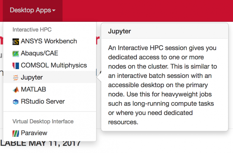
Install Julia kernel for Jupyter
Since version 1.0, OSC users must manage their own IJulia kernels in Jupyter. The following is an example of adding the latest version of IJulia and creating the corresponding version of the Julia kernel:
$ module load julia/1.0.5 $ create_julia_kernel Installing IJulia Resolving package versions... Updating `~/.julia/environments/v1.0/Project.toml` [7073ff75] + IJulia v1.23.2 Updating `~/.julia/environments/v1.0/Manifest.toml` ... ... IJulia installed: 1.23.2 [ Info: Installing Julia kernelspec in /users/PAS1234/username/.local/share/jupyter/kernels/julia-1.0
In Juptyer Notebook, you can find the item Julia 1.0.5 in the kernel list:
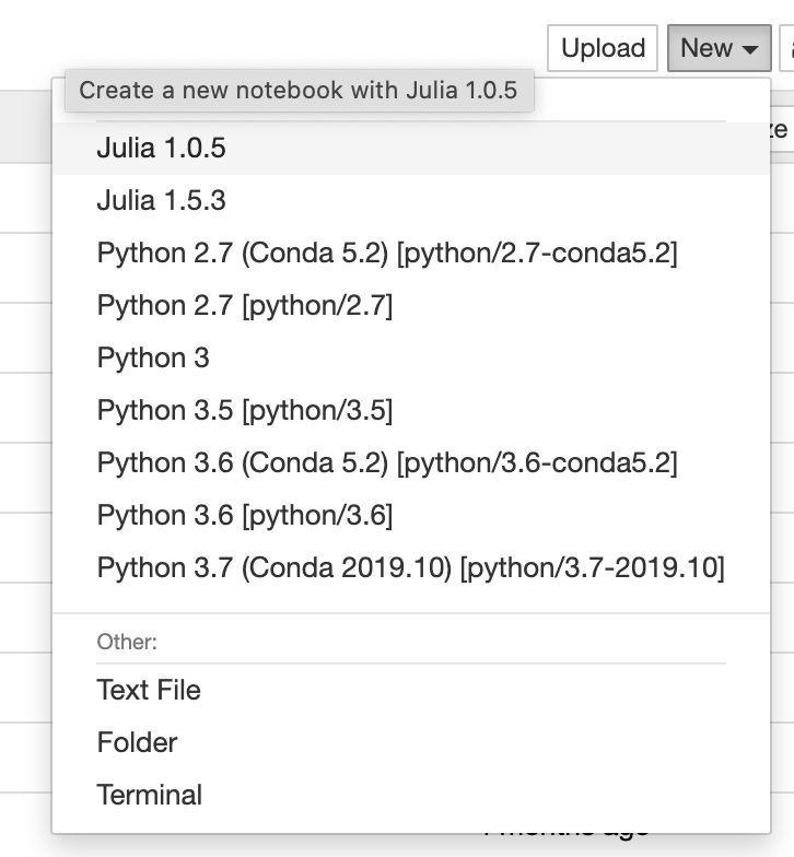
For more detail about package management, please refer to the Julia document.
Acess gurobi from Jupyter Notebook
To acess gurobi from Jupyter notebook, users would need to request access for the Gurobi software. More information can be found at Gurobi webpage. User would need to set the path to the gurobi license file located on Owens in the notebook as follows,
ENV["GRB_LICENSE_FILE"] = "/usr/local/gurobi/10.0.1/gurobi.lic"
Service:
Fields of Science:
Kallisto
Kallisto is an RNA-seq quantification program. It quantifies abundances of transcripts from RNA-seq data and uses psedoalignment to determine the compatibility of reads with targets, without needing alignment.
Availability and Restrictions
Versions
Kallisto is available on the Owens Clusters. The versions currently available at OSC are:
| Version | Owens |
|---|---|
| 0.43.1 | X* |
* Current Default Version
You can use module spider kallisto to view available modules for a given machine. Feel free to contact OSC Help if you need other versions for your work.
Access
Kallisto is available to all OSC users. If you have any questions, please contact OSC Help.
Publisher/Vendor/Repository and License Type
Nicolas Bray et al., Open source
Usage
Usage on Owens
Set-up
To configure your enviorment for use of Salmon, use command module load kallisto. This will load the default version.
Further Reading
Supercomputer:
Fields of Science:
LAMMPS
The Large-scale Atomic/Molecular Massively Parallel Simulator (LAMMPS) is a classical molecular dynamics code designed for high-performance simulation of large atomistic systems. LAMMPS generally scales well on OSC platforms, provides a variety of modeling techniques, and offers GPU accelerated computation.
Availability and Restrictions
Versions
LAMMPS is available on all clusters. The following versions are currently installed at OSC:
| Version | Owens | Pitzer | Ascend |
|---|---|---|---|
| 14May16 | P | ||
| 31Mar17 | PC | ||
| 16Mar18 | PC | ||
| 22Aug18 | PC | PC | |
| 5Jun19 | PC | PC | |
| 3Mar20 | PC* | PC* | |
| 29Oct20 | PC | PC | |
| 29Sep2021.3 | PC | PC | PC* |
| 20220623.1 | PC |
* Current default version; S = serial executables; P = parallel; C = CUDA
* IMPORTANT NOTE: You must load the correct compiler and MPI modules before you can load LAMMPS. To determine which modules you need, use
module spider lammps/{version}. Some LAMMPS versions are available with multiple compiler versions and MPI versions; in general, we recommend using the latest versions. (In particular, mvapich2/2.3.2 is recommended over 2.3.1 and 2.3; see the known issue.You can use module spider lammps to view available modules for a given machine. Feel free to contact OSC Help if you need other versions for your work.
Access
LAMMPS is available to all OSC users. If you have any questions, please contact OSC Help.
Publisher/Vendor/Repository and License Type
Sandia National Lab., Open source
Usage
Usage on Owens
Set-up
To load the default version of LAMMPS module and set up your environment, use
module load lammps . To select a particular software version, use module load lammps/version . For example, use module load lammps/14May16 to load LAMMPS version 14May16. Using LAMMPS
Once a module is loaded, LAMMPS can be run with the following command:
lammps < input.file
To see information on the packages and executables for a particular installation, run the module help command, for example:
module help lammps
Batch Usage
By connecting to owens.osc.edu you are logged into one of the login nodes which has computing resource limits. To gain access to the manifold resources on the cluster, you must submit your job to the batch system for execution. Batch jobs can request mutiple nodes/cores and compute time up to the limits of the OSC systems. Refer to Queues and Reservations and Batch Limit Rules for more info.
Interactive Batch Session
For an interactive batch session one can run the following command:
sinteractive -A <project-account> -N 1 -n 28 -g 1 -t 00:20:00
which requests one whole node with 28 cores ( -N 1 -n 28), for a walltime of 20 minutes ( -t 00:20:00 ), with one gpu (-g 1). You may adjust the numbers per your need.
Non-interactive Batch Job (Parallel Run)
A batch script can be created and submitted for a serial or parallel run. You can create the batch script using any text editor you like in a working directory on the system of your choice. Sample batch scripts and LAMMPS input files are available here:
~srb/workshops/compchem/lammps/
Below is a sample batch script. It asks for 56 processors and 10 hours of walltime. If the job goes beyond 10 hours, the job would be terminated.
#!/bin/bash #SBATCH --job-name=chain #SBATCH --nodes=2 --ntasks-per-node=28 #SBATCH --time=10:00:00 #SBATCH --account=<project-account> module load lammps sbcast -p chain.in $TMPDIR/chain.in cd $TMPDIR lammps < chain.in sgather -pr $TMPDIR $SLURM_SUBMIT_DIR/output
Usage on Pitzer
Set-up
To load the default version of LAMMPS module and set up your environment, use
module load lammps. Using LAMMPS
Once a module is loaded, LAMMPS can be run with the following command:
lammps < input.file
To see information on the packages and executables for a particular installation, run the module help command, for example:
module help lammps
Batch Usage
To access a cluster's main computational resources, you must submit your job to the batch system for execution. Batch jobs can request mutiple nodes/cores and compute time up to the limits of the OSC systems. Refer to Queues and Reservations and Batch Limit Rules for more info.
Interactive Batch Session
For an interactive batch session one can run the following command:
sinteractive -A <project-account> -N 1 -n 48 -g 1 -t 00:20:00
which requests one whole node with 28 cores ( -N 1 -n 48), for a walltime of 20 minutes ( -t 00:20:00 ), with one gpu (-g 1). You may adjust the numbers per your need.
Non-interactive Batch Job (Parallel Run)
A batch script can be created and submitted for a serial or parallel run. You can create the batch script using any text editor you like in a working directory on the system of your choice. Sample batch scripts and LAMMPS input files are available here:
~srb/workshops/compchem/lammps/
Below is a sample batch script. It asks for 56 processors and 10 hours of walltime. If the job goes beyond 10 hours, the job would be terminated.
#!/bin/bash #SBATCH --job-name=chain #SBATCH --nodes=2 --ntasks-per-node=48 #SBATCH --time=10:00:00 #SBATCH --account=<project-account> module load lammps sbcast -p chain.in $TMPDIR/chain.in cd $TMPDIR lammps < chain.in sgather -pr $TMPDIR $SLURM_SUBMIT_DIR/output
Known Issues
LAMMPS 14May16 velocity command problem on Owens
Updated: December 2016
Versions Affected: LAMMPS 14May16
Versions Affected: LAMMPS 14May16
LAMMPS 14May16 on Owens can hang when using the velocity command. Inputs that hang on Owens work on Oakley and Ruby. LAMMPS 31Mar17 on Owens also works. Here is an example failing input snippet:
velocity mobile create 298.0 111250 mom yes dist gaussian run 1000
Further Reading
Service:
Fields of Science:
LAPACK
LAPACK (Linear Algebra PACKage) provides routines for solving systems of simultaneous linear equations, least-squares solutions of linear systems of equations, eigenvalue problems, and singular value problems.
Availability and Restrictions
A highly optimized implementation of LAPACK is available on all OSC clusters as part of the Intel Math Kernel Library (MKL). We recommend that you use MKL rather than building LAPACK for yourself. MKL is available to all OSC users.
Publisher/Vendor/Repository and License Type
http://www.netlib.org/lapack/, Open source
Usage
See OSC's MKL software page for usage information. Note that there are lapack shared libraries on the clusters; however, these are old versions from the operating system and should generally not be used. You should modify your makefile or build script to link to the MKL libraries instead; a quick start for a crude approach is to merely load an mkl module and substitute the consequently defined environment variable $(MKL_LIBS) for -llapack.
Further Reading
Service:
Technologies:
Fields of Science:
LS-DYNA
LS-DYNA is a general purpose finite element code for simulating complex structural problems, specializing in nonlinear, transient dynamic problems using explicit integration. LS-DYNA is one of the codes developed at Livermore Software Technology Corporation (LSTC).
Availability and Restrictions
Versions
LS-DYNA is available on Owens Cluster for both serial (smp solver for single node jobs) and parallel (mpp solver for multipe node jobs) versions. The versions currently available at OSC are:
| Version | Owens | |
|---|---|---|
|
9.0.1 |
smp | X |
| mpp | X | |
| 10.1.0 | smp | X |
| mpp | X | |
| 11.0.0 | smp | X* |
| mpp | X* | |
| 12.1.0 | smp | X |
| mpp | X | |
* Current default version
You can use module spider ls-dyna to view available modules for a given machine. Feel free to contact OSC Help if you need other versions for your work.
Access for Academic Users
ls-dyna is available to academic OSC users with proper validation. In order to obtain validation, please contact OSC Help for further instruction.
Access for Commercial Users
Contact OSC Help for getting access to LS-DYNA if you are a commercial user.
Publisher/Vendor/Repository and License Type
LSTC, Commercial
Usage
Usage on Owens
Set-up on Owens
To view available modules installed on Owens, use module spider ls-dyna for smp solvers, and use module spider mpp for mpp solvers. In the module name, '_s' indicates single precision and '_d' indicates double precision. For example, mpp-dyna/971_d_9.0.1 is the mpp solver with double precision on Owens. Use module load name to load LS-DYNA with a particular software version. For example, use module load mpp-dyna/971_d_9.0.1 to load LS-DYNA mpp solver version 9.0.1 with double precision on Owens.
Batch Usage on Owens
When you log into owens.osc.edu you are actually logged into a linux box referred to as the login node. To gain access to the mutiple processors in the computing environment, you must submit your job to the batch system for execution. Batch jobs can request mutiple nodes/cores and compute time up to the limits of the OSC systems. Refer to Queues and Reservations and Batch Limit Rules for more info. Batch jobs run on the compute nodes of the system and not on the login node. It is desirable for big problems since more resources can be used.
Interactive Batch Session
For an interactive batch session one can run the following command:
sinteractive -A <project-account> -N 1 -n 28 -t 00:20:00 -L lsdyna@osc:28which requests one whole node with 28 cores (
-N 1 -n 28), for a walltime of 20 minutes (-t 00:20:00). You may adjust the numbers per your need.
Non-interactive Batch Job (Serial Run)
A batch script can be created and submitted for a serial or parallel run. You can create the batch script using any text editor you like in a working directory on the system of your choice. Please follow the steps below to use LS-DYNA via the batch system:
1) copy your input files (explorer.k in the example below) to your work directory at OSC
2) create a batch script, similar to the following file, saved as job.txt. It uses the smp solver for a serial job (nodes=1) on Owens:
#!/bin/bash #SBATCH --job-name=plate_test #SBATCH --time=5:00:00 #SBATCH --nodes=1 --ntasks-per-node=28 #SBATCH --account <project-account> #SBATCH -L lsdyna@osc:28 # The following lines set up the LSDYNA environment module load ls-dyna/971_d_9.0.1 # # Run LSDYNA (number of cpus > 1) # lsdyna I=explorer.k NCPU=28
3) submit the script to the batch queue with the command: sbatch job.txt.
When the job is finished, all the result files will be found in the directory where you submitted your job ($SLURM_SUBMIT_DIR). Alternatively, you can submit your job from the temporary directory ($TMPDIR), which is faster to access for the system and might be beneficial for bigger jobs. Note that $TMPDIR is uniquely associated with the job submitted and will be cleared when the job ends. So you need to copy your results back to your work directory at the end of your script.
Non-interactive Batch Job (Parallel Run)
Please follow the steps below to use LS-DYNA via the batch system:1) copy your input files (explorer.k in the example below) to your work directory at OSC
2) create a batch script, similar to the following file, saved as job.txt). It uses the mmp solver for a parallel job (nodes>1) on Owens:
#!/bin/bash #SBATCH --job-name=plate_test #SBATCH --time=5:00:00 #SBATCH --nodes=2 --ntasks-per-node=28 #SBATCH --account <project-account> #SBATCH -L lsdyna@osc:56 # The following lines set up the LSDYNA environment module load intel/18.0.3 module load intelmpi/2018.3 module load mpp-dyna/971_d_9.0.1 # # Run LSDYNA (number of cpus > 1) # srun mpp971 I=explorer.k NCPU=56
3) submit the script to the batch queue with the command: sbatch job.txt.
When the job is finished, all the result files will be found in the directory where you submitted your job ($SLURM_SUBMIT_DIR). Alternatively, you can submit your job from the temporary directory ($TMPDIR), which is faster to access for the system and might be beneficial for bigger jobs. Note that $TMPDIR is uniquely associated with the job submitted and will be cleared when the job ends. So you need to copy your results back to your work directory at the end of your script. An example scrip should include the following lines:
...
cd $TMPDIR
sbcast $SLURM_SUBMIT_DIR/explorer.k explorer
... #launch the solver and execute
sgather -pr $TMPDIR ${SLURM_SUBMIT_DIR}
#or you may specify a directory for your output files, such as
#sgather -pr $TMPDIR ${SLURM_SUBMIT_DIR}/output
Further Reading
- The LSDYNA homepage
- The LSDYNA users manual (structural and keyword editions)
- The LSDYNA Theory Manual
- The LS-PREPOST Tutorial
See Also
Supercomputer:
Service:
Fields of Science:
LS-OPT
LS-OPT is a package for design optimization, system identification, and probabilistic analysis with an interface to LS-DYNA.
Availability and Restrictions
Versions
The following versions of ls-opt are available on OSC clusters:
| Version | Owens |
|---|---|
| 6.0.0 | X* |
* Current default version
You can use module spider ls-opt to view available modules for a given machine. Feel free to contact OSC Help if you need other versions for your work.
Access
In order to use LS-OPT, you need LS-DYNA. ls-dyna is available to academic OSC users with proper validation. In order to obtain validation, please contact OSC Help for further instruction.
Publisher/Vendor/Repository and License Type
LSTC, Commercial
Usage
Usage on Owens
Set-up
To configure your environment for use of LS-OPT, run the following command:
module load ls-opt. The default version will be loaded. To select a particular LS-OPT version, use module load ls-opt/version. For example, use module load ls-opt/6.0.0 to load LS-OPT 6.0.0.Further Reading
Supercomputer:
Service:
LS-PrePost
LS-PrePost is an advanced pre and post-processor that is delivered free with LS-DYNA.
Availability and Restrictions
Versions
The following versions of ls-prepost are available on OSC clusters:
| Version | Owens |
|---|---|
| 4.6 | X* |
* Current default version
You can use module spider ls-prepost to view available modules for a given machine. Feel free to contact OSC Help if you need other versions for your work.
Access
In order to use LS-PrePost you need LS-DYNA. ls-dyna is available to academic OSC users with proper validation. In order to obtain validation, please contact OSC Help for further instruction.
Publisher/Vendor/Repository and License Type
LSTC, Commercial
Usage
Usage on Owens
Set-up
To configure your environment for use of LS-PrePost, run the following command:
module load ls-prepost. The default version will be loaded. To select a particular LS-PrePost version, use module load ls-prepost/<version>. For example, use module load ls-prepost/4.6 to load LS-PrePost 4.6.Further Reading
Supercomputer:
Service:
User-Defined Material for LS-DYNA
This page describes how to specify user defined material to use within LS-DYNA. The user-defined subroutines in LS-DYNA allow the program to be customized for particular applications. In order to define user material, LS-DYNA must be recompiled.
Usage
The first step to running a simulation with user defined material is to build a new executable. The following is an example done with solver version mpp971_s_R7.1.1.
When you log into the Oakley system, load mpp971_s_R7.1.1 with the command:
module load mpp-dyna/R7.1.1
Next, copy the mpp971_s_R7.1.1 object files and Makefile to your current directory:
cp /usr/local/lstc/mpp-dyna/R7.1.1/usermat/* $PWD
Next, update the dyn21.f file with your user defined material model subroutine. Please see the LS-DYNA User's Manual (Keyword version) for details regarding the format and structure of this file.
Once your user defined model is setup correctly in dyn21.f, build the new mpp971 executable with the command:
make
To execute a multi processor (ppn > 1) run with your new executable, execute the following steps:
1) move your input file to a directory on an OSC system (pipe.k in the example below)
2) copy your newly created mpp971 executable to this directory as well
3) create a batch script (lstc_umat.job) like the following:
#PBS -N LSDYNA_umat #PBS -l walltime=1:00:00 #PBS -l nodes=2:ppn=8 #PBS -j oe #PBS -S /bin/csh # This is the template batch script for running a pre-compiled # MPP 971 v7600 LS-DYNA. # Total number of processors is ( nodes x ppn ) # # The following lines set up the LSDYNA environment module load mpp-dyna/R7.1.1 # # Move to the directory where the job was submitted from # (i.e. PBS_O_WORKDIR = directory where you typed qsub) # cd $PBS_O_WORKDIR # # Run LSDYNA # NOTE: you have to put in your input file name # mpiexec mpp971 I=pipe.k NCPU=16
4) Next, submit this job to the batch queue with the command:
qsub lstc_umat.job
The output result files will be saved to the directory you ran the qsub command from (known as the $PBS_O_WORKDIR_
Documentation
On-line documentation is available on LSTC website.
See Also
Service:
MAGMA
MAGMA is a collection of next generation linear algebra (LA) GPU accelerated libraries designed and implemented by the team that developed LAPACK and ScaLAPACK. MAGMA is for heterogeneous GPU-based architectures, it supports interfaces to current LA packages and standards, e.g., LAPACK and BLAS, to allow computational scientists to effortlessly port any LA-relying software components. The main benefits of using MAGMA are that it can enable applications to fully exploit the power of current heterogeneous systems of multi/manycore CPUs and multi-GPUs, and deliver the fastest possible time to an accurate solution within given energy constraints.
Availability and Restrictions
Versions
MAGMA is available on Owens, and the following versions are currently available at OSC:
| Version | Owens |
|---|---|
| 2.2.0 | X(I)* |
* Current default version; I = avaible with only intel
You can use module spider magma to view available modules for a given machine. Feel free to contact OSC Help if you need other versions for your work.
Access for Academic Users
MAGMA is available to all OSC users. If you have any questions, please contact OSC Help.
Publisher/Vendor/Repository and License Type
Computational Algebra Group, Univ. of Sydney, Open source
Usage
Usage on Owens
Set-up
To load the default version of MAGMA module, cuda must first be loaded. Use
module load cuda toload the default version of cuda, or module load cuda/version to load a specific version. Then use module load magma to load MAGMA. To select a particular software version, use module load magma/version. For example, use module load magma/2.2.0 to load MAGMA version 2.2.0Using MAGMA
To run MAGMA in the command line, use the Intel compilers (icc, ifort).
icc $MAGMA_CFLAGS example.c
or
ifort $MAGMA_F90FLAGS example.F90
Batch Usage
When you log into owens.osc.edu you are actually logged into a linux box referred to as the login node. To gain access to the mutiple processors in the computing environment, you must submit your MAGMA simulation to the batch system for execution. Batch jobs can request mutiple nodes/cores and compute time up to the limits of the OSC systems. Refer to Queues and Reservations and Batch Limit Rules for more info.
Interactive Batch Session
For an interactive batch session, one can run the following command:sinteractive -A <account> -N 1 -n 28 -t 1:00:00which gives you 1 node and 28 cores (
-N 1 -n 28) with 1 hour (-t 1:00:00). You may adjust the numbers per your need.
Non-interactive Batch Job (Serial Run)
A batch script can be created and submitted for a serial or parallel run. You can create the batch script using any text editor you like in a working directory on the system of your choice.
Below is the example batch script (job.txt) for a serial run:
#!/bin/bash ## MAGMA Example Batch Script for the Basic Tutorial in the MAGMA manual #SBATCH --job-name=6pti #SBATCH --nodes=1 --ntasks-per-node=28 #SBATCH --time=0:20:00 #SBATCH --account <account> module load cuda module load magma # Use TMPDIR for best performance. cd $TMPDIR # SLURM_SUMIT_DIR refers to the directory from which the job was submitted. cp $SLURM_SUMIT_DIR/example.c . icc $MAGMA_CFLAGS example.c
In order to run it via the batch system, submit the job.txt file with the command: sinteractive job.txt.
Further Reading
Supercomputer:
Service:
Technologies:
Fields of Science:
MATLAB
MATLAB is a technical computing environment for high-performance numeric computation and visualization. MATLAB integrates numerical analysis, matrix computation, signal processing, and graphics in an easy-to-use environment where problems and solutions are expressed just as they are written mathematically--without traditional programming.
Availability and Restrictions
Versions
MATLAB is available on Pitzer and Owens Clusters. The versions currently available at OSC are:
| Version | Owens | Pitzer | Notes |
|---|---|---|---|
| r2015b | X | ||
| r2016b | X | ||
| r2017a | X | ||
| r2018a | X | X | |
| r2018b | X | X | |
| r2019a | X | ||
| r2019b | X | X | |
| r2020a | X* | X* | |
| r2021b | X | X | |
| r2022a | X | X | |
| r2023a | X | X | |
| r2023b | X | X | |
| r2024a | X | X |
* Current default version
You can use module spider matlab to view available modules for a given machine. Feel free to contact OSC Help if you need other versions for your work.
Access: Academic Users Only (non-commercial, non-government)
Academic users can use Matlab at OSC. All users must be added to the license server before using MATLAB. Please contact OSC Help to be granted access or for any license related questions.
Publisher/Vendor/Repository and License Type
MathWorks, Commercial (University site license)
Toolboxes and Features
OSC's current licenses support the following MATLAB toolboxes and features (please contact OSC Help for license-specific questions):
MATLAB Simulink 5G Toolbox AUTOSAR Blockset Aerospace Blockset Aerospace Toolbox Antenna Toolbox Audio Toolbox Automated Driving Toolbox Bioinformatics Toolbox Communications Toolbox Computer Vision Toolbox Control System Toolbox Curve Fitting Toolbox DDS Blockset DSP System Toolbox Data Acquisition Toolbox Database Toolbox Datafeed Toolbox Deep Learning HDL Toolbox Deep Learning Toolbox Econometrics Toolbox Embedded Coder Filter Design HDL Coder Financial Instruments Toolbox Financial Toolbox Fixed-Point Designer Fuzzy Logic Toolbox GPU Coder Global Optimization Toolbox HDL Coder HDL Verifier Image Acquisition Toolbox Image Processing Toolbox Instrument Control Toolbox LTE Toolbox Lidar Toolbox MATLAB Coder MATLAB Compiler SDK MATLAB Compiler MATLAB Report Generator Mapping Toolbox Mixed-Signal Blockset Model Predictive Control Toolbox Model-Based Calibration Toolbox Motor Control Blockset Navigation Toolbox OPC Toolbox Optimization Toolbox Parallel Computing Toolbox Partial Differential Equation Toolbox Phased Array System Toolbox Powertrain Blockset Predictive Maintenance Toolbox RF Blockset RF PCB Toolbox RF Toolbox ROS Toolbox Radar Toolbox Reinforcement Learning Toolbox Risk Management Toolbox Robotics System Toolbox Robust Control Toolbox Satellite Communications Toolbox Sensor Fusion and Tracking Toolbox SerDes Toolbox Signal Integrity Toolbox Signal Processing Toolbox SimBiology SimEvents Simscape Driveline Simscape Electrical Simscape Fluids Simscape Multibody Simscape Simulink 3D Animation Simulink Check Simulink Code Inspector Simulink Coder Simulink Compiler Simulink Control Design Simulink Coverage Simulink Design Optimization Simulink Design Verifier Simulink Desktop Real-Time Simulink PLC Coder Simulink Real-Time Simulink Report Generator Simulink Requirements Simulink Test SoC Blockset Spreadsheet Link Stateflow Statistics and Machine Learning Toolbox Symbolic Math Toolbox System Composer System Identification Toolbox Text Analytics Toolbox UAV Toolbox Vehicle Dynamics Blockset Vehicle Network Toolbox Vision HDL Toolbox WLAN Toolbox Wavelet Toolbox Wireless HDL Toolbox
See this page if you need to install additional toolbox by yourself.
Usage
Usage on Owens
Set-up
To load the default version of MATLAB module, use
module load matlab . For a list of all available MATLAB versions and the format expected, type: module spider matlab . To select a particular software version, use module load matlab/version . For example, use module load matlab/r2015b to load MATLAB version r2015b. Running MATLAB
The following command will start an interactive, command line version of MATLAB:
matlab -nodisplayIf you are able to use X-11 forwarding and have enabled it in your SSH client software preferences, you can run MATLAB using the GUI by typing the command
matlab . For more information about the matlab command usage, type matlab –h for a complete list of command line options.
The commands listed above will run MATLAB on the login node you are connected to. As the login node is a shared resource, running scripts that require significant computational resources will impact the usability of the cluster for others. As such, you should not use interactive MATLAB sessions on the login node for any significant computation. If your MATLAB script requires significant time, CPU power, or memory, you should run your code via the batch system.
Batch Usage
When you log into owens.osc.edu you are actually logged into a Linux box referred to as the login node. To gain access to the multiple processors in the computing environment, you must submit your job to the batch system for execution. Batch jobs can request multiple nodes/cores and compute time up to the limits of the OSC systems. Refer to Queues and Reservations and Batch Limit Rules for more info.
Interactive Batch Session
For an interactive batch session using the command line version of MATLAB, one can run the following command:sinteractive -A <project-account> -N 1 -n 28 -t 00:20:00
which requests one whole node with 28 cores ( -N 1 -n 28 ), for a walltime of 20 minutes ( -t 00:20:00 ). Here you can run MATLAB interactively by loading the MATLAB module and running MATLAB with the options of your choice as described above. You may adjust the numbers per your need.
Usage on Pitzer
Set-up
To load the default version of MATLAB module, use
module load matlab.Running MATLAB
The following command will start an interactive, command line version of MATLAB:
matlab -nodisplayIf you are able to use X-11 forwarding and have enabled it in your SSH client software preferences, you can run MATLAB using the GUI by typing the command
matlab. For more information about the matlab command usage, type matlab –h for a complete list of command line options.
The commands listed above will run MATLAB on the login node you are connected to. As the login node is a shared resource, running scripts that require significant computational resources will impact the usability of the cluster for others. As such, you should not use interactive MATLAB sessions on the login node for any significant computation. If your MATLAB script requires significant time, CPU power, or memory, you should run your code via the batch system.
Batch Usage
When you log into pitzer.osc.edu you are actually logged into a Linux box referred to as the login node. To gain access to the multiple processors in the computing environment, you must submit your job to the batch system for execution. Batch jobs can request multiple nodes/cores and compute time up to the limits of the OSC systems. Refer to Queues and Reservations and Batch Limit Rules for more info.
Interactive Batch Session
For an interactive batch session using the command line version of MATLAB, one can run the following command:sinteractive -A <project-account> -N 1 -n 40 -t 00:20:00
which requests one whole node with 40 cores ( -N 1 -n 40), for a walltime of 20 minutes ( -t 00:20:00 ). Here you can run MATLAB interactively by loading the MATLAB module and running MATLAB with the options of your choice as described above. You may adjust the numbers per your need.
Additional Topics
MATLAB Parallel Functions and Tools
MATLAB now supports Parallel Computing Toolbox. The Parallel Computing Toolbox lets you solve computationally and data-intensive programs using multiple cores and GPUs. Built in MATLAB functions and tools allow for easy parallelization of MATLAB applications. Programs can be run both interactively or as batch jobs.
Currently only r2019b and newer versions have full support for the Parallel Computing Toolbox on Owens and Pitzer.
Please refer to the official MATLAB documentation for more information on the Parallel Computing Toolbox
Sections:
Creating Parallel Pools
You can parallelize by requesting a certain number of workers and then work can be offloaded onto those pool of workers. For local computations, the number of workers you can requests relates to the number of cores available.
To start up a pool you can run:
p = gcp
p is the pool object which can be used to check information on the worker pool.
By default gcp creates a pool of workers equal to the number of cores on the job.
Note:
- It may takes a couple of seconds to a minute to start up a pool.
- You cannot run multiple parallel pools at the same time on a single job.
To delete the current pool if one exists run:
delete(gcp('nocreate')
After the program is done running the pool will still remain active. MATLAB only deletes the pool after the default 30 minutes. So if you want to end a pool you must manually delete it, let MATLAB timeout the pool. or terminate the job. If you make changes to the code interactively it is recommended you delete the pool and spin up a new pool of workers.
See Matlab documentation for more information on worker pools here
Parpool and Batch
Parallel jobs can also be submitted by a Matlab script, as is demonstrated below in the Submitting Single-Node Parallel MATLAB Jobs and Submitting Multi-Node Parallel MATLAB Jobs sections. The 2 main ways of doing so is through parpool and batch.
First, before using parpool or batch, you must get a handle to the profile cluster. To do this use the parcluster function.
% creates cluster profile object for the specified cluster profile
c = parcluster("Cluster_Profile");
% creates a cluster object to your current job
c = parcluster("local");
See the Submitting Multi-Node Parallel MATLAB Jobs section below for more information on how to create a cluster profile.
Creating the object with a cluster profile will result in a new job to be submitted when launching parpool or batch. Make sure the appropriate arguments are set in the cluster profile. Creating the object with the 'local' parameter will not result in a new job to be launched when executing parpool or batch. Instead the workers will be allocated to the cores in your current job.
Once you have you a profile object created, you can now launch parallel jobs.
To launch a parpool parallel job, simply run:
p = parpool(c, 40); % c: is the cluster profile object initialized using parcluster % 40: because we want 40 workers
Important Note: You can only run one parpool job at a time. You need to make sure the parent job which launched the parpool job has a long enough wall time to accommodate the new job otherwise the parpool job will get terminated when the parent job ends.
To launch a batch job:
job1 = batch(c, @function, 1, {"arg1", "arg2"}, "Pool", 40); % launch batch job of 40 workers
% c: is the cluster profile object initialized using parcluster
wait(job1); % wait for job to finish
X = fetchOutputs(job1); %retrieve the output data from job
%job detail can be accessed by the job1 object including its status.
Here we launched a batch job to exectute @function. @function will be run on a parallel pool of 40 workers.
Since batch does not block up your matlab program, you wan use the wait function to wait for your batch job(s) to finish before proceeding. The fetchOutputs function can be used to retrieve the outputs of the batch job.
The notable difference between parpool and batch is that you can run multiple batch jobs at a time and their duration is not tied to the parent job (the parent job can finish executing and the batch jobs will continue executing unlike parpool).
Please See the Running Concurrent Jobs section if running multiple jobs at the same time
please refer to the official MATLAB documentation for more details: parcluster parpool batch
Parfor
To parallelize a for-loop you can use a parfor-loop.
A parfor-loop will run the different iterations of the loop in parallel by assigning the iterations to the workers in the pool. If multiple jobs are assigned to a worker then those jobs will be competed in serial by the worker. It is important to carefully assess and make good judgment calls on how many workers you want to request for the job.
To utilize a parfor-loop simply replace the for in a standard for-loop with parfor.
%converting a standard for loop to a parfor looks as such:
for i=1:10
%loop code
end
%replace the for with parfor
parfor i=1:10
%loop code
end
Important note: parfor may complete the iterations out of order, so it is important that the iterations are not order dependent.
A parfor-loop is run synchronously, thus the MATLAB process is halted until all tasks for the workers are settled.
Important Limitations:
- Cannot nest parfors inside of one another: This is because workers cannot start or access further parallel pools.
- parfor-loops and for-loops can be nested inside one another (it is often a judgment call on whether it is better to nest a parfor inside a for-loop or vice versa).
%valid
for i=1:10
parfor j=1:10
%code
end
end
%invalid: will throw error
parfor i=1:10
parfor j=1:10
%code
end
end
- Cannot have loop elements dependent on other iterations
- Since, there is not guaranteed order of completion of iterations in a parfor-loop and workers cannot communicate with each other, each loop iteration must be independent.
A = ones(1,100);
parfor i = 1:100
A(i) = A(i-1) + 1; %invalid iteration entry as the current iteration is dependent on the previous iteration
end
- step size must be 1
parfor i = 0:0.1:1 %invalid because step side is not 1
%code
end
To learn more about par-for loops see the official matlab parfor documentation
Parfeval
Another way to run loops in parallel in MATLAB is to use parfeval loops. When using parfeval to run functions in the background it creates an object called a future for each function and adds the future object to a poll queue.
First, initialize a futures object vector with the number of expected futures. Preallocation of the futures vector is not required, but is highly recommended to increase efficiency: f(1:num_futures) = parallel.FevalFuture;
For each job, you can fill the futures vector with an instance of the future. Filling the vector allows you to get access to the futures later. f(index) = parfeval(@my_function, numOutputs, input1, input2);
@my_functionis the pointer to the function I want to runnumOutputsis the integer represented number of returned outputs you need frommy_function. Note: this does not need to match the actual number for outputs the function returns.input1, input2, ...is the parameter list formy_function
%example code f(1:10) = parallel.FevalFuture; for i = 1:10 f(i) = parfeval(@my_function, 1, 2); end
when a future is created, it is added to a queue. Then the workers will takes futures from the queue to begin to evaluate them.
you can use the state property of a future to find out whether it is queued, running, or finished: f(1).State
you can manually cancel a future by running: cancel(f(1));
you can block off MATLAB until a certain future complete by using: wait(f(4));
when a future is finished you can check its error message is one was thrown by: f(1).Error.message
You can cancel all running and/or queued futures by (p is the parallel pool object):
cancel(p.FevalQueue.QueuedFutures); cancel(p.FevalQueue.RunningFutures);
Processing worker outputs as they complete
One of the biggest strengths of parfeval is its ability to run futures asynchronously (runs in the background without blocking the Matlab program). This allows you to fetch results from the futures as they get completed.
p = gcp; %luanch parallel pool with number of workers equal to availble cores
f(1:10) = parallel.FevalFuture; % initalize futures vector
for k = 1:10
f(k) = parfeval(@rand, 1, 1000, 1); % lanch 10 futures which will run in background on parallel pool
end
results = cell(1,10); % create a results vector
for k = 1:10
[completedK, value] = fetchNext(f); % fetch the next worker that finished and print its results
results{completedK} = value;
fprintf("got result with index: %d, largest element in vector is %f. \n", completedK, max(results{completedK}));
end
In this example above, as each @rand future gets completed by the workers, the fetchNext retrieves the returned data.
MATLAB also provides functions such at afterEach and afterAll to process the outputs as workers complete futures.
Please refer to the official MATLAB documentation for more information on parfeval: parfeval and parfeval parallel pooling
Spmd
spmd stands for Single Program Multiple Data. The spmd block can be used to execute multiple blocks of data across multiple workers. Here is a simple example:
delete(gcp('nocreate')); %delete a parallel pool if one is already spun up
p = parpool(2); %create a pool of 2 workers
spmd
fprintf("worker %d says hello world", spmdIndex); %have each worker print statement
end
%end of code
%output Worker 1: worker 1 says hello world Worker 2: worker 2 says hello world %end of output
The spmdIndex variable can be used to access the index of each worker. spmd also allows for communication between workers via sending and receiving data. Additionally, data can be received by the MATLAB client from the workers. For more information on spmd and its functionality vist the Official MATLAB documentation
Submitting Single-Node Parallel MATLAB Jobs
When parallelizing on a single node, you can generate and run a parallel pool on the same node as the current job or interactive secession.
Here is an example MATLAB script of submitting a parallel job to a single node:
p = parcluster('local');
% open parallel pool of 8 workers on the cluster node
parpool(p, 8);
spmd
% assign each worker a print function
fprintf("Worker %d says Hello", spmdIndex);
end
delete(gcp); % close the parallel pool
exit
Since we will only be using a single node, we will use the 'local' cluster profile. This will create a profile object p which will be the cluster profile of the job the command was run in. We also set the pool size be less than or equal to the number of cores on our compute node; In this case we will used 8. See cluster specifications to see the maximum number of cores on a single node for each cluster.
Now lets save this MATLAB script as "wokrer_hello.m" and write a Slurm batch script to submit and execute it as a job. "worker_hello.slurm" slurm script:
#!/bin/bash #SBATCH --job-name=worker_hello # job name #SBATCH --cpus-per-task=8 # 8 cores #SBATCH --output=worker_hello.log # set output file #SBATCH --time=00:10:00 # 10 minutes wall time # load Matlab module module load matlab/r2023a cd $SLURM_SUBMIT_DIR #run matlab script matlab -nodisplay -r worker_hello
In this script first we set a MATLAB module to the module path, in this example its MATLAB/r2023a. Then we make a call to execute the "worker_hello.m" MATLAB script. The -nodisplay flag is to prevent matlab from attempting to launch a GUI. In this script we requested 8 cores since our MATLAB script uses 8 workers. When performing single node parallelizations be mindful of the max number of cores each node has on the different clusters.
Then the job was submitted using sbatch -A <project-account> worker_hello.slurm through the command line.
The output was then generated into the "worker_hello.log" file:
< M A T L A B (R) >
Copyright 1984-2023 The MathWorks, Inc.
R2023a Update 2 (9.14.0.2254940) 64-bit (glnxa64)
April 17, 2023
To get started, type doc.
For product information, visit www.mathworks.com.
Starting parallel pool (parpool) using the 'Processes' profile ...
Connected to parallel pool with 8 workers.
Worker 1:
Worker 1 says Hello
Worker 2:
Worker 2 says Hello
Worker 3:
Worker 3 says Hello
Worker 4:
Worker 4 says Hello
Worker 5:
Worker 5 says Hello
Worker 6:
Worker 6 says Hello
Worker 7:
Worker 7 says Hello
Worker 8:
Worker 8 says Hello
Parallel pool using the 'Processes' profile is shutting down.
As we see a total of 8 workers were created and each printed their message in parallel.
Create Cluster Profile
Before we can parallelize matlab across multiple nodes we need to create a cluster profile. In the profile we can specify any arguments and adjust the settings of submitting jobs through MATLAB.
If you are running matlab r2019b and newer you can run configCluster to configure matlab with the profile of the cluster your job is running on:
configCluster % configer matlab with profile c = parcluster; % get a handle to cluster profile % set any additional properties c.AdditionalProperties.WallTime = '00:10:00'; % set wall time to 10 mintues c.AdditionalProperties.AccountName = 'PZS1234' % set account name c.saveProfile % locally save the profile
When creating a profile you must set the
AccountName and WallTime and make sure to save the profile.
If the above method does not work, or you prefer to to use the GUI, then you can configure a cluster profile from the GUI. You must be running MATLAB r2023a and newer versions to be able to search for OSC's clusters.
1. First we need to launch a Matlab GUI through onDemand. See onDemand for more details.
2. Next within the MATLAB GUI, navigate to HOME->Environment->Parallel->Discover Clusters:
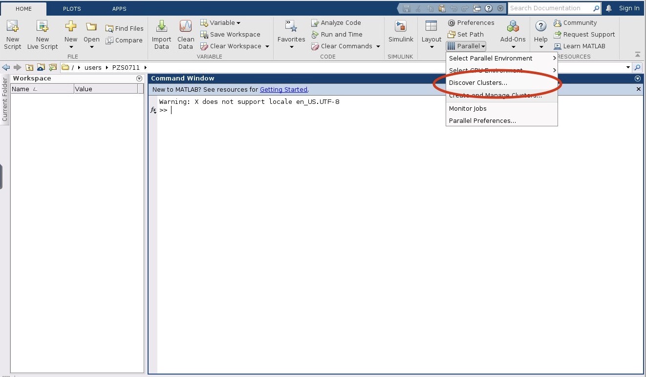
3. Then check the "On your network" box. Then click Next.
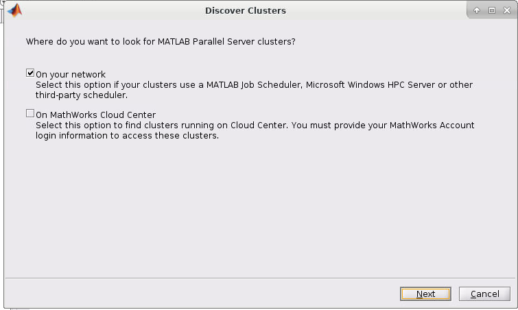
4. If you started the Matlab GUI though onDemand then you should see the cluster of the session listed as such (I started mine through Pitzer so Pitzer is listed):
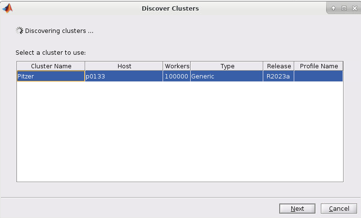
5. Now select the cluster and click Next. You should now have a screen like this:
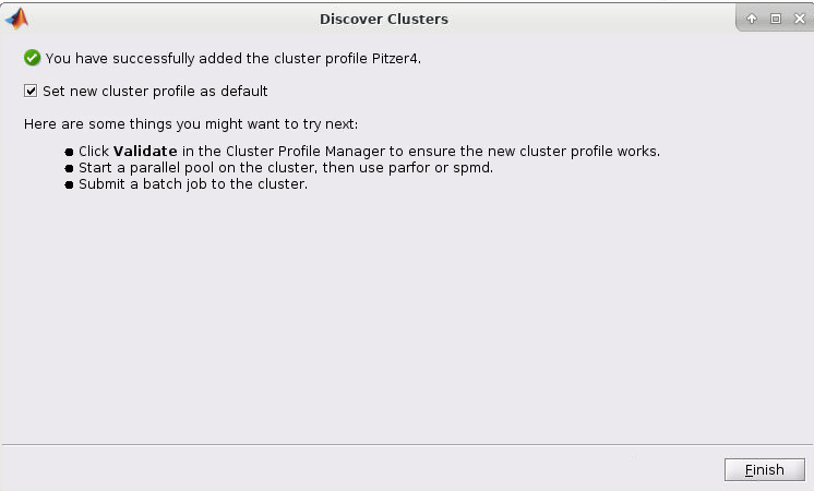
6. Now check the "Set new cluster profile as default" box and then click Finish
7. Now if you click on HOME->Environment->Parallel->Select Parallel Environment you will be presented with a list of profiles available which you can toggle between. Your new profile that was just created should be listed.
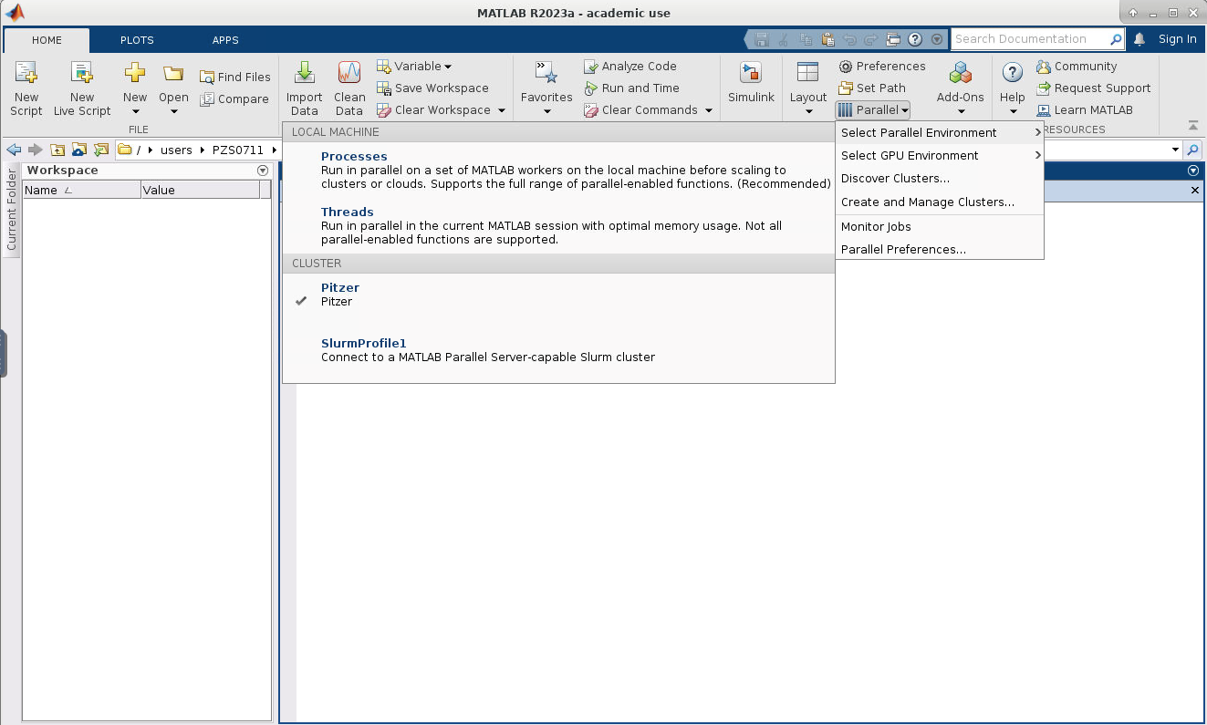
8. Now we need to edit the cluster profile to suit the needs of the job we want to submit. Go to HOME->Environment->Parallel->Create and Manage Clusters. Select the cluster profile you want to edit and then click edit. Most settings can be left as default but the following must be set: the AccountName and WallTime under the SCHEDULER PLUGIN must be set to your account name:
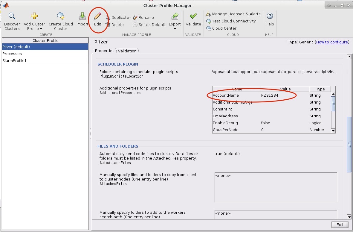
If you want MATLAB to submit jobs with slurm parameters other than the default you may edit them in this menu.
When creating a profile you must set the
AccountName and WallTime Validating Profile
If you run into any issues using your cluster profile you may want to validate your profile. Validating is not required, but may help debug any profile related issues.
To validate a profile:
- Within the MATLAB GUI, navigate to HOME->Environment->Parallel->Create and Manage Clusters:
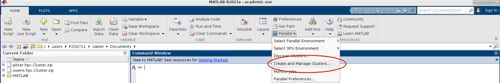
- Select the profile you want to validate on the left side of the menu. Then select the Validation tab next to the Properties tab. Now in the Number of worker to use: box specifiy the number of cores you are using to run the OnDemand MATLAB GUI on. If you leave the box blank, then it will run the tests with more workers then cores available to your matlab session which will result in a failed validation.
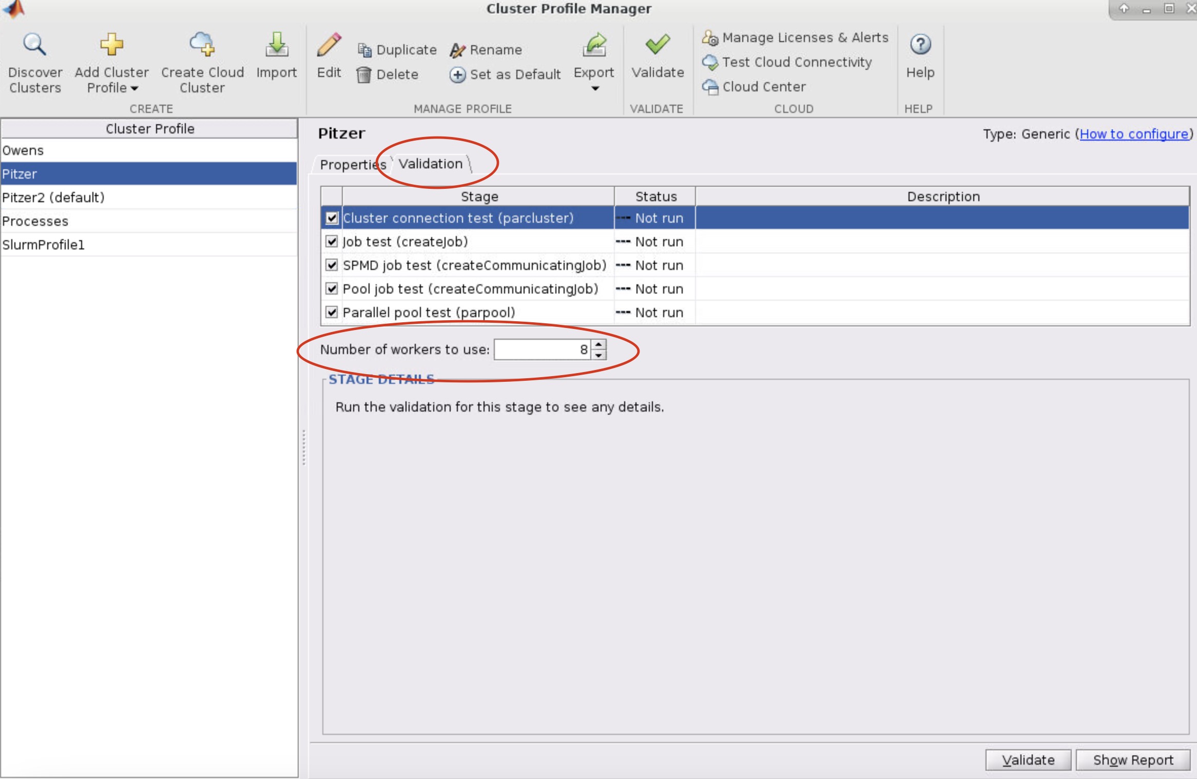
-
Next, click validate in the bottom right or top of the menu
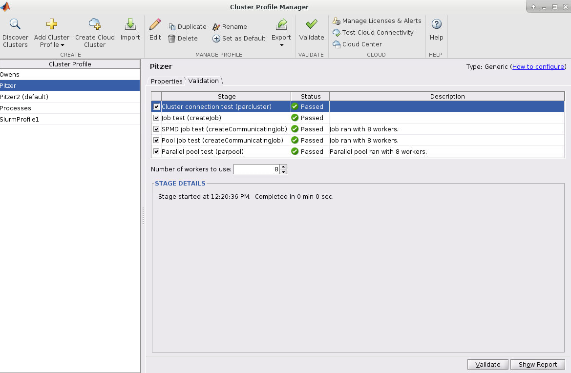
Make sure the
AccountName and WallTime are both set in the cluster profile before validating! Make sure the number of worker used for validation is less than or equal to the number of cores available to the MATLAB session!Submitting Multi-Node Parallel MATLAB Jobs
Before Submitting multi-node parallel jobs you must create a cluster profile. See Create Cluster Profile section above.
Now let's create a submit a multi-node parallel MATLAB job. Here is a matlab script:
configCluster % configer matlab with profile
p = parcluster; % get a handle to cluster profile
% set any additional properties
p.AdditionalProperties.WallTime = '00:10:00'; % set wall time to 10 mintues
p.AdditionalProperties.AccountName = 'PZS1234' % set account name
p.saveProfile % locally save the profile
% if profile created using the "Discover Clusters" from the GUI then you can simply run: p = parcluster('Pitzer'); instead of the above code.
% open parallel pool of 80 workers
parpool(p, 80); % you must specify the number of workers you want
spmd
fprintf("Worker %d says Hello", spmdIndex);
end
delete(gcp); % close the parallel pool
exit
In this example we opened a cluster profile called 'Pitzer'. This profile name should be the same as the cluster profile created above. We then launched another job using the parpool function with 80 workers onto the Pitzer cluster with the default settings (wall-time was set to 1 minutes instead of the default 1 hour). Since 80 workers is over the maximum number of cores per node, the Pitzer profile created using the steps above will automatically request 2 nodes for the job to accomodate the workers.
This script was saved in a file called "hello_multi_node.m".
Now a slurm script was created as follows:
#!/bin/bash #SBATCH --job-name=hello_multi_node # job name #SBATCH --cpus-per-task=1 # 1 cores #SBATCH --output=hello_multi_node.log # set output file #SBATCH --time=00:10:00 # 10 minutes wall time # load Matlab module module load matlab/r2023a cd $SLURM_SUBMIT_DIR #run matlab script matlab -nodisplay -r hello_multi_node
This job was allocated only 1 core. This is because the "hello_multi_node.m" will launch another job on the Pitzer cluster when calling parpool to exectute the parallel workers. Since the main entry matlab program does not need multiple nodes, we only allocated 1.
Then the job was submitted using sbatch -A <project-account> hello_multi_node.slurm through the command line.
The output was then generated into the "hello_multi_node.log" file:
< M A T L A B (R) >
Copyright 1984-2023 The MathWorks, Inc.
R2023a Update 2 (9.14.0.2254940) 64-bit (glnxa64)
April 17, 2023
To get started, type doc.
For product information, visit www.mathworks.com.
Starting parallel pool (parpool) using the 'Pitzer' profile ...
additionalSubmitArgs =
'--ntasks=80 --cpus-per-task=1 --ntasks-per-node=40 -N 2 --ntasks-per-core=1 -A PZS0711 --mem-per-cpu=4gb -t 00:01:00'
Connected to parallel pool with 80 workers.
Worker 1:
Worker 1 says hello
Worker 2:
Worker 2 says hello
Worker 3:
Worker 3 says hello
Worker 4:
Worker 4 says hello
Worker 5:
Worker 5 says hello
.
.
.
Worker 80:
Worker 80 says hello
Notice by the additionalSubmitArgs = line another job was launched with 2 nodes with 40 cores on each node. It is in this new job that the workers completed their tasks.
In this example we used parpool to launch a new parallel job, but batch can also be used. See MATLAB Parallel Functions and Tools for more information on the batch function
You can modify the properties of a cluster profile through code aswell through the c.AdditionalProperties attribute. This is helpful if you want to submit multiple batch jobs through a single Matlab program with different submit arguments.
c = parcluster('Pitzer'); % get cluster object
c.AdditionalProperties.WallTime = "00:15:00"; % sets the wall time to the c cluster object. Does not change the 'Pitzer' profile itself, only the local object.
c.saveProfile; % saves to the central 'Pitzer' profile.
Multithreading
Multithreading allows some functions in MATLAB to distribute the work load between cores of the node that your job is running on. By default, all of the current versions of MATLAB available on the OSC clusters have multithreading enabled.
The system will run as many threads as there are cores on the nodes requested.
Multithreading increases the speed of some linear algebra routines, but if you would like to disable multithreading you may include the option " -singleCompThread" when running MATLAB. An example is given below:
#!/bin/bash #SBATCH --job-name disable_multithreading #SBATCH --time=00:10:00 #SBATCH --nodes=1 --ntasks-per-node=40 #SBATCH --account=<project-account> module load matlab matlab -singleCompThread -nodisplay -nodesktop < hello.m # end of example file
Using GPU in MATLAB
A GPU can be utilized for MATLAB. You can acquire a GPU for the job by
#SBATCH --gpus-per-node=1
for Owens, or Pitzer. For more detail, please read here.
You can check the GPU assigned to you using:
gpuDeviceCount # show how many GPUs you have gpuDevice # show the details of the GPU
To utilize a GPU, you will need to transfer the data from a standard CPU array to a GPU array. gpuArrays are a data structure which is stored on the GPU. Make sure the GPU has enough memory to hold this data. Even if the gpuArray fits in the GPU memory, make sure that any temporary arrays and data generated will also be able to fit on the GPU.
To create a GPU array:
X = [1,2,3]; %create a standard array G = gpuArray(X); %transfer array over to gpu
To check if data is stored on the GPU run:
isgpuarray(G); %returns true or false
To transfer the GPU data back onto the host memory use:
Y = gather(G);
Note:
- To reduce overhead time, limit the amount of data transfers between the host memory and GPU memory. For instance, many MATLAB functions allow you to create data directly on the GPU by specify the "gpuArray" parameter:
gpu_matrix = rand(N, N, "gpuArray"); - Gathering data from gpuArrays can be costly in terms of time and thus it is generally not necessary to gather the data unless you need to store it or the data needs processing to through non-gpu compatible functions.
When you have data in a GPU Array there are many built-in MATLAB functions which can run on the data. See list on the MATLAB website for a full list of compatible functions.
For more information about GPU programming for MATLAB, please read GPU Computing from Mathworks.
Running Concurrent Jobs
Concurrent jobs on OSC clusters
When you run multiple jobs concurrently, each job will try to access your preference files at the same time. It may create a race condition issue and may cause a negative impact on the system and the failure of your jobs. In order to avoid this issue, please add the following in your job script:
export MATLAB_PREFDIR=$TMPDIR
It will reset the preference directory to the local temporary directory, $TMPDIR. If you wish to start your Matlab job with the preference files you already have, add the following before you change MATLAB_PREFDIR.
cp -a ~/.matlab/{matlab version}/* $TMPDIR/
If you use matlab/r2020a, your matlab version is "R2020a".
References
- Official PDF documentation can be obtained from the MathWorks Website.
- Using MatLab's Parallel Server for multi-core and multi-node jobs.
Service:
Fields of Science:
SPM
SPM is made freely available to the [neuro]imaging community, to promote collaboration and a common analysis scheme across laboratories. The software represents the implementation of the theoretical concepts of Statistical Parametric Mapping in a complete analysis package.
The SPM software is a suite of MATLAB (MathWorks) functions and subroutines with some externally compiled C routines. SPM was written to organise and interpret our functional neuroimaging data. The distributed version is the same as that we use ourselves.
Availability and Restrictions
Versions
The following versions are available on OSC clusters:
|
VERSION |
Pitzer |
|---|---|
| 8 |
X |
| 12.7771 | X* |
* Current default version
spm/12.7771 comes with CONN 0.19 and xjview 9.7
spm/8 comes with CONN 0.19, xjview 9.7, and Marsbar 0.44
You can use module spider spm to view available modules for a given machine. Feel free to contact OSC Help if you need other versions for your work.
Access
SPM is available to all OSC users. If you have any questions, please contact OSC Help.
Publisher/Vendor/Repository and License Type
SPM is free but copyright software, distributed under the terms of the GNU General Public Licence as published by the Free Software Foundation (either version 2, as given in file LICENCE.txt, or at your option, any later version). Further details on "copyleft" can be found at https://www.gnu.org/copyleft/. In particular, SPM is supplied as is. No formal support or maintenance is provided or implied.
Usage
Usage on Pitzer
Set-up
To configure your environment for use of SPM, run the following command: module load spm. The default version will be loaded. To select a particular AFNI version, use module load spm/version. For example, use module load spm/12.7771 to load SPM/12.7771.
SPM is a MATLAB suite, so you need to load MATLAB before you can use SPM:
module load matlab/r2020a module load spm/12.7771 or module load matlab/r2020a module load spm/8
Note that spm/12.7771 comes with CONN 0.19 and xjview 9.7, and spm/8 comes with CONN 0.19, xjview 9.7, and Marsbar 0.44. Marsbar 0.44 doesn't support spm/12.7771.
Further Reading
Supercomputer:
Service:
Fields of Science:
MIRA
MIRA - Sequence assembler and sequence mapping for whole genome shotgun and EST / RNASeq sequencing data. Can use Sanger, 454, Illumina and IonTorrent data. PacBio: CCS and error corrected data usable, uncorrected not yet.
Availability and Restrictions
Versions
The following versions of MIRA are available on OSC clusters:
| Version | Owens |
|---|---|
| 4.0.2 | X* |
* Current default version
You can use module spider mira to view available modules for a given machine. Feel free to contact OSC Help if you need other versions for your work.
Access
MIRA is available to all OSC users. If you have any questions, please contact OSC Help.
Publisher/Vendor/Repository and License Type
Bastien Chevreux, Open source
Usage
Usage on Owens
Set-up
To configure your environment for use of MIRA, run the following command:
module load mira. The default version will be loaded. To select a particular MIRA version, use module load mira/version. For example, use module load mira/4.0.2 to load MIRA 4.0.2.Further Reading
Supercomputer:
Service:
Fields of Science:
MKL - Intel Math Kernel Library
Intel Math Kernel Library (MKL) consists of high-performance, multithreaded mathematics libraries for linear algebra, fast Fourier transforms, vector math, and more.
Availability and Restrictions
Versions
OSC supports single-process use of MKL for LAPACK and BLAS levels one through three. For multi-process applications, we also support the ScaLAPACK, FFTW2, and FFTW3 MKL wrappers. MKL modules are available for the Intel, GNU, and PGI compilers. MKL is available on Pitzer, Ruby, and Owens Clusters. The versions currently available at OSC are:
| Version | Owens | Pitzer | Notes |
|---|---|---|---|
| 11.3.2 | X | ||
| 11.3.3 | X | ||
| 2017.0.2 | X | ||
| 2017.0.4 | X | ||
| 2017.0.7 | X | ||
| 2018.0.3 | X | X | |
| 2019.0.3 | X | X | |
| 2019.0.5 | X* | X* | |
| 2021.3.0 | X | X |
* Current Default Version
You can use module spider mkl to view available modules for a given machine. Feel free to contact OSC Help if you need other versions for your work.
Access
MKL is available to all OSC users.
Publisher/Vendor/Repository and License Type
Intel, Commercial
Usage
Usage on Owens
Set-up
To load the default MKL, run the following command: module load mkl. To load a particular version, use module load mkl/version. For example, use module load mkl/11.3.3 to load MKL version 11.3.3. You can use module spider mkl to view available modules.
This step is required for both building and running MKL applications. Note that loading an mkl module defines several environment variables that can be useful for compiling and linking to MKL, e.g., MKL_CFLAGS and MKL_LIBS.
Exception: The "mkl" module is usually not needed when using the Intel compilers; just use the "-mkl" flag on the compile and link steps.
Usage on Pitzer
Set-up
To load the default MKL, run the following command: module load mkl.
This step is required for both building and running MKL applications. Note that loading an mkl module defines several environment variables that can be useful for compiling and linking to MKL, e.g., MKL_CFLAGS and MKL_LIBS.
Exception: The "mkl" module is usually not needed when using the Intel compilers; just use the "-mkl" flag on the compile and link steps.
Dynamic Linking Variables
These variables indicate how to link to MKL. While their contents are used during compiling and linking, the variables themselves are usually specified during the configuration stage of software installation. The form of specification is dependent on the application software. For example, some softwares employing cmake for configuration might use this form:
cmake .. -DMKL_INCLUDE_DIR="$MKLROOT/include" -DMKL_LIBRARIES="MKL_LIBS_SEQ"
Here is an exmple for some software employing autoconf:
./configure --prefix=$HOME/local/pkg/version CPPFLAGS="$MKL_CFLAGS" LIBS="$MKL_LIBS" LDFLAGS="$MKL_LIBS"
| Variable | Comment |
|---|---|
| MKL_LIBS | Link with parallel threading layer of MKL |
| GNU_MKL_LIBS | Dedicated for GNU compiler in Intel programming environment |
| MKL_LIBS_SEQ | Link with sequential threading layer of MKL |
| MKL_SCALAPACK_LIBS | Link with BLACS and ScaLAPACK of MKL |
| MKL_CLUSTER_LIBS | Link with BLACS, CDFT and ScaLAPACK of MKL |
Further Reading
Tag:
Service:
Fields of Science:
MRIQC
MRIQC is a program that provides automatic prediction of quality and visual reporting of MRI scans.
Availability and Restrictions
Versions
The following versions are available on OSC clusters:
| Version | Pitzer |
|---|---|
| 0.16.1 | X* |
| 23.1.0rc0 | X |
* Current default version
You can use module spider mriqc to view available modules for a given machine. Feel free to contact OSC Help if you need other versions for your work.
Access
MRIQC is available to all OSC users. If you have any questions, please contact OSC Help.
Publisher/Vendor/Repository and License Type
MRIQC uses the 3-clause BSD license; the full license is in the file LICENSE in the mriqc distribution. Open-source.
All trademarks referenced herein are property of their respective holders.
Copyright (c) 2015-2017, the mriqc developers and the CRN. All rights reserved.
Usage
Usage on Pitzer
Set-up
To configure your environment for use of mriqc, run the following command: module load mriqc. The default version will be loaded. To select a particular MRIQC version, use module load mriqc/version. For example, use module load mriqc/0.16.1 to load MRIQC 0.16.1.
MRIQC is installed in a singularity container. MRIQC_IMG environment variable contains the container image file path. So, an example usage would be
module load mriqc singularity exec $MRIQC_IMG mriqc --version
For more information about singularity usages, please read OSC singularity page.
Further Reading
Tag:
Supercomputer:
Service:
Fields of Science:
MRIcroGL
MRIcroGL is medical image viewer that allows you to load overlays (e.g. statistical maps), draw regions of interest (e.g. create lesion maps).
Availability and Restrictions
Versions
MRIcroGL is available on Pitzer cluster. These are the versions currently available:
| Version | Pitzer | Notes |
|---|---|---|
| 1.2.20220720 | X* |
* Current default version
You can use module spider mricrogl to view available modules for a given machine. Feel free to contact OSC Help if you need other versions for your work.
Access
mricrogl is available to all OSC users. Please review the license before you use.
Publisher/Vendor/Repository and License Type
The Software has been developed for research purposes only and is not a clinical tool.
Copyright (c) 2014-2019 Chris Rorden. All rights reserved.
See more about the license for MRIcroGL at the GitHub repository here.
Usage
Usage on Pitzer
Set-up
To configure your environment for use of MRIcroGL, run the following command: module load mricrogl. The default version will be loaded.
MRIcroGL is a GUI based software, so it requires an x11 connection. You can read about it from here for more details, but the simplest way to access the GUI is by using the OnDemand portal. Once you have an x11 connection, you can open the GUI by doing the following:
$ module load mricrogl $ mricrogl.sif
MRIcroGL is installed in an apptainer container. For more information about apptainer usages, please read OSC apptainer page.
Further Reading
Supercomputer:
MUSCLE
MUSCLE is a program for creating multiple alignments of protein sequences.
Availability and Restrictions
Versions
The following versions of bedtools are available on OSC clusters:
| Version | Owens | Pitzer |
|---|---|---|
| 3.8.31 | X* | X* |
* Current default version
You can use module spider muscle to view available modules for a given machine. Feel free to contact OSC Help if you need other versions for your work.
Access
MUSCLE is available to all OSC users. If you have any questions, please contact OSC Help.
Publisher/Vendor/Repository and License Type
Public domain software.
Usage
Usage on Owens
Set-up
To configure your environment for use of metilene, run the following command:
module load muscle. The default version will be loaded. To select a particular MUSCLE version, use module load muscle/version. For example, use module load muscle/3.8.31 to load MUSCLE 3.8.31.Usage on Pitzer
Set-up
To configure your environment for use of metilene, run the following command:
module load muscle. The default version will be loaded. To select a particular MUSCLE version, use module load muscle/version. For example, use module load muscle/3.8.31 to load MUSCLE 3.8.31.Further Reading
Service:
Fields of Science:
MVAPICH2
MVAPICH2 is a standard library for performing parallel processing using a distributed-memory model.
Availability and Restrictions
Versions
The following versions of MVAPICH2 are available on OSC systems:
| Version | Owens | Pitzer | Ascend |
|---|---|---|---|
| 2.3 | X | X | |
| 2.3.1 | X | X | |
| 2.3.2 | X | X | |
| 2.3.3 | X* | X* | |
| 2.3.5 | X | X | |
| 2.3.6 | X | X | X |
| 2.3.7 | X* |
* Current default version
You can use module spider mvapich2 to view available modules for a given machine. Feel free to contact OSC Help if you need other versions for your work.
Access
MPI is available to all OSC users. If you have any questions, please contact OSC Help.
Publisher/Vendor/Repository and License Type
NBCL, The Ohio State University/ Open source
Usage
Set-up
To set up your environment for using the MPI libraries, you must load the appropriate module:
module load mvapich2
You will get the default version for the compiler you have loaded.
Note:Be sure to swap the intel compiler module for the gnu module if you're using gnu.
Building With MPI
To build a program that uses MPI, you should use the compiler wrappers provided on the system. They accept the same options as the underlying compiler. The commands are shown in the following table.
| C | mpicc |
| C++ | mpicxx |
| FORTRAN 77 | mpif77 |
| Fortran 90 | mpif90 |
For example, to build the code my_prog.c using the -O2 option, you would use:
mpicc -o my_prog -O2 my_prog.c
In rare cases you may be unable to use the wrappers. In that case you should use the environment variables set by the module.
| Variable | Use |
|---|---|
$MPI_CFLAGS |
Use during your compilation step for C programs. |
$MPI_CXXFLAGS |
Use during your compilation step for C++ programs. |
$MPI_FFLAGS |
Use during your compilation step for Fortran 77 programs. |
$MPI_F90FLAGS |
Use during your compilation step for Fortran 90 programs. |
$MPI_LIBS |
Use when linking your program to the MPI libraries. |
For example, to build the code my_prog.c without using the wrappers you would use:
mpicc -c $MPI_CFLAGS my_prog.cmpicc -o my_prog my_prog.o $MPI_LIBS
Batch Usage
Programs built with MPI can only be run in the batch environment at OSC. For information on starting MPI programs using the srun or mpiexec command, see Batch Processing at OSC.
Be sure to load the same compiler and mvapich modules at execution time as at build time.
Known Issues
Large MPI job startup failure
Updated: Nov 2019
Versions Affected: Mvapich2/2.3 & 2.3.1
Versions Affected: Mvapich2/2.3 & 2.3.1
We have found that large MPI jobs may hang at startup with mvapich2/2.3 and mvapich/2.3.1 (on any compiler dependency) due to a known bug that has been fixed in release 2.3.2. If users experience this issue, please switch to mvapich2/2.3.2
Further Reading
- The Message Passing Interface (MPI) Standard
- MPI Training Course
See Also
Service:
Technologies:
Fields of Science:
Mathematica
Mathematica is a mathematical computation program. It is capable in many areas of technical computing including but not limited to neural networks, machine learning, image processing, geometry, data science and visualizations.
Availability and Restrictions
Versions
Mathematica is available on the Pitzer and Owens Clusters. The versions currently available at OSC are:
| Owens | Pitzer | |
|---|---|---|
| 13.2.1 | X | X |
You can use module spider mathematica to view available modules for a given machine. Feel free to contact OSC Help if you need other versions for your work.
Access for Academic Users
Use of Mathematica is open to academic Ohio State University users. OSC does not provide Mathematica licenses for outside of Ohio State University due to licensing restrictions. All users must be added to the system before using Mathematica. Please contact OSC Help to be granted access or for any license related questions.
Publisher/Vendor/Repository and License Type
Mathematica, commercial
Usage
Usage on Owens
Set-up on Owens
To load the default version of Mathematica module, use module load mathematica/13.2.1.
Running Mathematica
To run Mathematica, you should log into your osc account for OSC OnDemand. Then at the top of your screen navigate to the Interactive Apps dropdown menu. There you may select Mathematica and launch the task. After the application is available you can open and use Mathematica.
Alternatively, you may request an OSC OnDemand desktop and load Mathematica with the command module load mathematica/13.2.1. Then you can run Mathematica by typing the command mathematica
The command listed below will run Mathematica on the login node you are connected to. As the login node is a shared resource, running scripts that require significant computational resources will impact the usability of the cluster for others. As such, you should not use interactive Mathematica sessions on the login node for any significant computation. If your Mathematica script requires significant time, CPU power, or memory, you should run your code via the batch system.
Usage on Pitzer
Set-up on Pitzer
To load the default version of Mathematica module, use module load mathematica/13.2.1.
Running Mathematica
To run Mathematica, you should log into your osc account for OSC OnDemand. Then at the top of your screen navigate to the Interactive Apps dropdown menu. There you may select Mathematica and launch the task. After the application is available you can open and use Mathematica.
Alternatively, you may request an OSC OnDemand desktop and load Mathematica with the command module load mathematica/13.2.1. Then you can run Mathematica by typing the command mathematica
The command listed below will run Mathematica on the login node you are connected to. As the login node is a shared resource, running scripts that require significant computational resources will impact the usability of the cluster for others. As such, you should not use interactive Mathematica sessions on the login node for any significant computation. If your Mathematica script requires significant time, CPU power, or memory, you should run your code via the batch system.
Running Mathematica jobs with GPU
A GPU can be utilized for Mathematica. You can acquire a GPU for the job by
#SBATCH --gpus-per-node=1
for Owens, or Pitzer. If running with an OnDemand desktop, select a GPU node to launch the desktop on. For more detail, please read here.
For more information about GPU computing for Mathematica, please read GPU Computing from Wolfram.
Further Reading
Service:
Fields of Science:
Miniconda3
Miniconda3 is a free minimal installer for conda. It is a small, bootstrap version of Anaconda that includes only conda, Python, the packages they depend on, and a small number of other useful packages, including pip, zlib and a few others.
Availability and Restrictions
Versions
Miniconda is available on the Ascend Cluster. The versions currently available at OSC are:
| Version | Owens | Pitzer | Ascend |
|---|---|---|---|
| 4.10.3 | X* | ||
| 4.10.3-py37 | X* | X* | |
| 4.12.0-py38 | X | X | |
| 4.12.0-py39 | X | X | |
| 23.3.1-py310 | X | X |
* Current Default Version
You can use module spider miniconda3 to view available modules for a given machine. Feel free to contact OSC Help if you need other versions for your work.
Access
Miniconda3 is available to all OSC users. If you have any questions, please contact OSC Help.
Publisher/Vendor/Repository and License Type
Conda, Free use and redistribution under the terms of the EULA for Miniconda.
Usage
Tag:
MotionCor2
MotionCor2 uses multi-GPU acceleration to correct anisotropic cryo-electron microscopy images at the single pixel level across the whole frame, making it suitable for single particle and tomographic images. Iterative, patch-based motion detection is combined with spatial and temporal constraints and dose weighting.
Availability and Restrictions
Versions
The following versions are available on OSC clusters:
| Version | Pitzer |
|---|---|
| 1.4.4 | X* |
* Current default version
You can use module spider motioncor2 to view available modules for a given machine. Feel free to contact OSC Help if you need other versions for your work.
Access
MotionCor2 is available to academic/non-profit OSC users. Please review the vendor's webpage and the attached license agreement below before use. If you have any questions, please contact OSC Help.
Publisher/Vendor/Repository and License Type
University of California San Francisco, License Agreement attached below.
Usage
Usage on Pitzer
Set-up
To configure your environment for use of motioncor2, run the following command: module load motioncor2. The default version will be loaded. To select a particular scipion version, use module load motioncor2/version. For example, use module load motioncor2/1.4.4 to load MotionCor2.1.4.4.
Further Reading
Documentation Attachment:
Supercomputer:
Service:
Technologies:
Fields of Science:
MuTect
MuTect is a method developed at the Broad Institute for the reliable and accurate identification of somatic point mutations in next generation sequencing data of cancer genomes.
Availability and Restrictions
Versions
The following versions of MuTect are available on OSC clusters:
| Version | Owens |
|---|---|
| 1.1.7 | X* |
* Current default version
You can use module spider mutect to view available modules for a given machine. Feel free to contact OSC Help if you need other versions for your work.
Access for Academic Users
MuTect is available to academic OSC users. Please review the license agreement carefully before use. If you have any questions, please contact OSC Help.
Publisher/Vendor/Repository and License Type
The Broad Institute, Inc./ Freeware (academic)
Usage
Usage on Owens
Set-up
To configure your environment for use of MuTect, run the following command:
module load mutect. The default version will be loaded. To select a particular MuTect version, use module load mutect/version. For example, use module load mutect/1.1.4 to load MuTect 1.1.4.NOTE: Java 1.7.0 will also need to be loaded in order to use MuTect:
module load java/1.7.0.Usage
This software is a Java executable .jar file; thus, it is not possible to add to the PATH environment variable.
From module load mutect, a new environment variable, MUTECT, will be set.
Thus, users can use the software by running the following command: java -jar $MUTECT {other options}.
Further Reading
Supercomputer:
Service:
Fields of Science:
NAMD
NAMD is a parallel molecular dynamics code designed for high-performance simulation of large biomolecular systems. NAMD generally scales well on OSC platforms and offers a variety of modelling techniques. NAMD is file-compatible with AMBER, CHARMM, and X-PLOR.
Availability and Restrictions
Versions
The following versions of NAMD are available:
| Version | Owens | Pitzer |
|---|---|---|
| 2.11 | X | |
| 2.12 | X | |
| 2.13b2 | X | |
| 2.13 | X* | X* |
* Current default version
* IMPORTANT NOTE: You need to load correct compiler and MPI modules before you use NAMD. In order to find out what modules you need, use
module spider namd/{version} .You can use module spider namd to view available modules for a given machine. Feel free to contact OSC Help if you need other versions for your work.
Access
NAMD is available to all OSC users for academic purpose.
Publisher/Vendor/Repository and License Type
TCBG, University of Illinois/ Open source (academic)
Usage
Set-up
To load the NAMD software on the system, use the following command: module load namd/"version" where "version" is the version of NAMD you require. The following will load the default or latest version of NAMD: module load namd .
Using NAMD
NAMD is rarely executed interactively because preparation for simulations is typically performed with extraneous tools, such as, VMD.
Batch Usage
Sample batch scripts and input files are available here:
~srb/workshops/compchem/namd/
The simple batch script for Owens below demonstrates some important points. It requests 56 processors and 2 hours of walltime. If the job goes beyond 2 hours, the job would be terminated.
#!/bin/bash
#SBATCH --job-name apoa1
#SBATCH --nodes=2 --ntasks-per-node=28
#SBATCH --time=2:00:00
#SBATCH --account=<project-account>
module load intel/18.0.4
module load mvapich2/2.3.6
module load namd
# SLURM_SUBMIT_DIR refers to the directory from which the job was submitted.
for FILE in *
do
sbcast -p $FILE $TMPDIR/$FILE
done
# Use TMPDIR for best performance.
cd $TMPDIR
run_namd apoa1.namd
sgather -pr $TMPDIR $SLURM_SUBMIT_DIR/output
Or equivalently, on Pitzer:
#!/bin/bash
#SBATCH --job-name apoa1
#SBATCH --nodes=2 --ntasks-per-node=48
#SBATCH --time=2:00:00
#SBATCH --account=<project-account>
module load intel/18.0.4
module load mvapich2/2.3.6
module load namd
# SLURM_SUBMIT_DIR refers to the directory from which the job was submitted.
# the following loop assumes you have the necessary .namd, .pdb, .psf, and .xplor files
# in the directory you are submitting the job from
for FILE in *
do
sbcast -p $FILE $TMPDIR/$FILE
done
# Use TMPDIR for best performance.
cd $TMPDIR
run_namd apoa1.namd
sgather -pr $TMPDIR $SLURM_SUBMIT_DIR/output
NOTE: ntaks-per-node should be a maximum of 28 on Owens and maximum of 48 on Pitzer.
GPU support
We have GPU support with NAMD 2.12 for Owens clusters. These temporarily use pre-compiled binaries due to installation issues. For more detail, please read the corresponding example script:
~srb/workshops/compchem/namd/apoa1.namd212nativecuda.owens.pbs # for Owens
Further Reading
Service:
Fields of Science:
NBO
The Natural Bond Orbital (NBO) program is a discovery tool for chemical insights from complex wavefunctions. NBO is a broad suite of 'natural' algorithms for optimally expressing numerical solutions of Schrödinger's wave equation in the chemically intuitive language of Lewis-like bonding patterns and associated resonance-type 'donor-acceptor' interactions.
Availability and Restrictions
Versions
NBO is available on Owens. The versions currently available at OSC are
| Version | Owens |
|---|---|
| 6.0 | X* |
* Current default version
You can use module spider nbo to view available modules for a given machine. Feel free to contact OSC Help if you need other versions for your work.
Access for Academic Users
NBO is available to non-commercial users; simply contact OSC Help to request the appropriate form for access.
Publisher/Vendor/Repository and License Type
University of Wisconsin System on behalf of the Theoretical Chemistry Institute, Non-Commercial
Usage
Usage on Owens
To set up your environment for NBO load one of its modulefiles:
module load nbo/6.0
For documentation corresponding to a loaded version, see $OSC_NBO_HOME/man/. Below is an example batch script that uses the i8 executables of NBO 6.0. This script specifies the Bash shell; for C type shells convert the export command to setenv syntax. The i4 executables are also installed and may be required by some quantum chemistry packages, e.g., ORCA as of Oct 2019. You can find other example inputs in ~srb/workshops/compchem/, such as ~srb/workshops/compchem/gaussian/nbo6.*.
#!/bin/bash # Example NBO 6.0 batch script. #SBATCH --job-name nbo-ch3nh2 #SBATCH --mail-type=ALL,END #SBATCH --time=0:10:00 #SBATCH --nodes=1 --ntasks-per-node=1 #SBATCH --account <account> qstat -f $SLURM_JOB_ID export module load nbo/6.0 module list cd $SLURM_SUBMIT_DIR pbsdcp --preserve ch3nh2.47 $TMPDIR cd $TMPDIR export NBOEXE=$OSC_NBO_HOME/bin/nbo6.i8.exe gennbo.i8.exe ch3nh2.47 ls -l pbsdcp --preserve --gather --recursive '*' $SLURM_SUBMIT_DIR
Further Reading
Supercomputer:
Service:
Fields of Science:
NCL/NCARG
NCAR Graphics is a Fortran and C based software package for scientific visualization. NCL (The NCAR Command Language), is a free interpreted language designed specifically for scientific data processing and visualization. It is a product of the Computational & Information Systems Laboratory at the National Center for Atmospheric Research (NCAR) and sponsored by the National Science Foundation. NCL has robust file input and output: it can read and write netCDF-3, netCDF-4 classic, HDF4, binary, and ASCII data, and read HDF-EOS2, GRIB1, and GRIB2. The graphics are based on NCAR Graphics.
Availability and Restrictions
Versions
NCL/NCAR Graphics is available on Pitzer and Owens Cluster. The versions currently available at OSC are:
| Version | Owens | Pitzer | Notes |
|---|---|---|---|
| 6.3.0 | X(GI) | ||
| 6.5.0 | X(GI) | X(GI) | netcdf-serial and hdf5-serial required for NCL |
| 6.6.2 | X(GI)* | X(GI)* | netcdf-serial and hdf5-serial required for NCL |
* Current default version; G = available with gnu; I = available with intel
You can use module spider ncarg to view available NCL/NCAR Graphics modules. Feel free to contact OSC Help if you need other versions for your work.
Access
NCL/NCAR Graphics is available for use by all OSC users.
Publisher/Vendor/Repository and License Type
University Corporation for Atmospheric Research, Open source
Usage
Usage on Owens
Set-up on Owens
To load the default version usemodule load ncarg. To select a particular version, use module load ncarg/version. For example, use module load ncarg/6.3.0 to load NCARG version 6.3.0 on Owens. For the default version of ncarg, use
module load ncarg
Batch Usage on Owens
Batch jobs can request mutiple nodes/cores and compute time up to the limits of the OSC systems. Refer to Queues and Reservations for Owens and Scheduling Policies and Limits for more info.
Interactive Batch Session
For an interactive batch session on Owens, one can run the following command:
sinterative -A <project-account> -N 1 -n 28 -t 1:00:00
which gives you one node and 28 cores (
-N 1 -n 28) with 1 hour (-t 1:00:00). You may adjust the numbers per your need.Non-interactive Batch Job (Serial Run)
A batch script can be created and submitted for a serial or parallel run. You can create the batch script using any text editor you like in a working directory on the system of your choice. The following example batch script file will use the input file named
interp1d_1.ncl.Below is the example batch script
job.txt for a serial run:#!/bin/bash #SBATCH --time=1:00:00 #SBATCH --nodes=1 --ntasks-per-node=28 #SBATCH --job-name=job-name #SBATCH --account <project-account> module load ncarg cp interp1d_1.ncl $TMPDIR cd $TMPDIR ncl interp1d_1.ncl pbsdcp --gather --recursive --preserve '*' interp1d.ps $SLURM_SUBMIT_DIR
In order to run it via the batch system, submit the job.txt file with the following command:
sbatch job.txt
Usage on Pitzer
Set-up on Pitzer
To load the default version usemodule load ncarg.
module load ncarg
Batch Usage on Pitzer
Batch jobs can request mutiple nodes/cores and compute time up to the limits of the OSC systems.
Interactive Batch Session
For an interactive batch session on Pitzer, one can run the following command:
sinteractive -A <project-account> -N 1 -n 48 -t 1:00:00
which gives you 1 node (
-N 1), 48 cores (-n 48), and 1 hour (-t 1:00:00). You may adjust the numbers per your need.Non-interactive Batch Job (Serial Run)
A batch script can be created and submitted for a serial or parallel run. You can create the batch script using any text editor you like in a working directory on the system of your choice. The following example batch script file will use the input file named
interp1d_1.ncl.Below is the example batch script
job.txt for a serial run:#!/bin/bash #SBATCH --time=1:00:00 #SBATCH --nodes=1 --ntasks-per-ndoe=48 #SBATCH --job-name=jobname #SBATCH --account <project-account> module load ncarg module load netcdf module load hdf5 cp interp1d_1.ncl $TMPDIR cd $TMPDIR ncl interp1d_1.ncl pbsdcp --gather --recursive --preserve '*' $SLURM_SUBMIT_DIR
In order to run it via the batch system, submit the job.txt file with the following command:
sbatch job.txt
Further Reading
Official documentation can be obtained from NCL homepage.
Service:
Fields of Science:
NWChem
NWChem aims to provide its users with computational chemistry tools that are scalable both in their ability to treat large scientific computational chemistry problems efficiently, and in their use of available parallel computing resources from high-performance parallel supercomputers to conventional workstation clusters.
Availability and Restrictions
Versions
The following versions of NWChem are available on OSC clusters:
| Version | Owens | Pitzer |
|---|---|---|
| 6.6 | X | |
| 6.8 | X | X |
| 7.0 | X* | X* |
* Current default version
You can use module spider nwchem to view available modules for a given machine. Feel free to contact OSC Help if you need other versions for your work.
Access
NWChem is available to all OSC users. If you have any questions, please contact OSC Help.
Publisher/Vendor/Repository and License Type
EMSL, Pacific Northwest National Lab., Open source
Usage
Usage on Owens
Set-up
To configure your environment for use of NWChem, run the following command:
module load nwchem. The default version will be loaded. To select a particular NWChem version, use module load nwchem/version. For example, use module load nwchem/6.6 to load NWChem 6.6.Usage on Pitzer
Set-up
To configure your environment for use of NWChem, run the following command:
module load nwchem. The default version will be loaded. Further Reading
Service:
Fields of Science:
Ncview
Ncview is a visual browser for netCDF format files. Typically you would use ncview to get a quick and easy, push-button look at your netCDF files. You can view simple movies of the data, view along various dimensions, take a look at the actual data values, change color maps, invert the data, etc.
Availability and Restrictions
Versions
The following versions of Ncview are available on OSC clusters:
| Version | Owens | Pitzer |
|---|---|---|
| 2.1.7 | X* | X* |
* Current default version
You can use module spider ncview to view available modules for a given machine. Feel free to contact OSC Help if you need other versions for your work.
Access
Ncview is available to all OSC users. If you have any questions, please contact OSC Help.
Publisher/Vendor/Repository and License Type
David W. Pierce, Open source
Usage
Usage on Owens
Set-up
To configure your environment for use of Ncview, run the following command: module load ncview. The default version will be loaded. To select a particular Ncview version, use module load ncview/version. For example, use module load ncview/2.1.7 to load Ncview 2.1.7.
Usage on Pitzer
Set-up
To configure your environment for use of Ncview, run the following command: module load ncview. The default version will be loaded. To select a particular Ncview version, use module load ncview/version. For example, use module load ncview/2.1.7 to load Ncview 2.1.7.
Further Reading
Service:
Fields of Science:
NetCDF
NetCDF (Network Common Data Form) is an interface for array-oriented data access and a library that provides an implementation of the interface. The netcdf library also defines a machine-independent format for representing scientific data. Together, the interface, library, and format support the creation, access, and sharing of scientific data.
Availability and Restrictions
Versions
NetCDF is available on Pitzer and Owens Clusters. The versions currently available at OSC are:
| Version | Owens | Pitzer | Ascend |
|---|---|---|---|
| 4.3.3.1 | X | ||
| 4.6.1 | X | X | |
| 4.6.2 | X | X | |
| 4.7.4 | X* | X* | |
| 4.8.1 | X* |
* Current default version
You can use module spider netcdf to view available modules for a given machine. Feel free to contact OSC Help if you need other versions for your work.
Additionally, the C++ interface version 4.3.0 and the Fortran interface version 4.4.2 is included in the netcdf/4.3.3.1 module.
Access
NetCDF is available to all OSC users. If you have any questions, please contact OSC Help.
Publisher/Vendor/Repository and License Type
University Corporation for Atmospheric Research, Open source
Usage
Usage on Owens
Set-up
Initalizing the system for use of the NetCDF is dependent on the system you are using and the compiler you are using. To load the default NetCDF, run the following command: module load netcdf. To use the parallel implementation of NetCDF, run the following command instead: module load pnetcdf. To load a particular version, use module load netcdf/version. For example, use module load netcdf/4.3.3.1 to load NetCDF version 4.3.3.1. You can use module spider netcdf to view available modules.
Building With NetCDF
With the netcdf library loaded, the following environment variables will be available for use:
| Variable | Use |
|---|---|
| $NETCDF_CFLAGS | Use during your compilation step for C or C++ programs. |
| $NETCDF_FFLAGS | Use during your compilation step for Fortran programs. |
| $NETCDF_LIBS | Use when linking your program to NetCDF. |
Similarly, when the pnetcdf module is loaded, the following environment variables will be available:
| VARIABLE | USE |
|---|---|
| $PNETCDF_CFLAGS | Use during your compilation step for C programs. |
| $PNETCDF_FFLAGS | Use during your compilation step for Fortran programs. |
| $PNETCDF_LIBS | Use when linking your program to NetCDF. |
For example, to build the code myprog.c with the netcdf library you would use:
icc -c $NETCDF_CFLAGS myprog.c icc -o myprog myprog.o $NETCDF_LIBS
Batch Usage
When you log into owens.osc.edu you are actually logged into a linux box referred to as the login node. To gain access to the mutiple processors in the computing environment, you must submit your job to the batch system for execution. Batch jobs can request mutiple nodes/cores and compute time up to the limits of the OSC systems. Refer to Queues and Reservations and Batch Limit Rules for more info.
Non-interactive Batch Job (Serial Run)
A batch script can be created and submitted for a serial or parallel run. You can create the batch script using any text editor you like in a working directory on the system of your choice. You must load the netcdf or pnetcdf module in your batch script before executing a program which is built with the netcdf library. Below is the example batch script that executes a program built with NetCDF:#!/bin/bash #SBATCH --job-name=job-name #SBATCH --nodes=1 --ntasks-per-node=28 #SBATCH --account <project-account> module load netcdf cp foo.dat $TMPDIR cd $TMPDIR appname < foo.dat > foo.out cp foo.out $SLURM_SUBMIT_DIR
Usage on Pitzer
Set-up
Initalizing the system for use of the NetCDF is dependent on the system you are using and the compiler you are using. To load the default NetCDF, run the following command: module load netcdf.
Building With NetCDF
With the netcdf library loaded, the following environment variables will be available for use:
| VARIABLE | USE |
|---|---|
| $NETCDF_CFLAGS | Use during your compilation step for C or C++ programs. |
| $NETCDF_FFLAGS | Use during your compilation step for Fortran programs. |
| $NETCDF_LIBS | Use when linking your program to NetCDF. |
Similarly, when the pnetcdf module is loaded, the following environment variables will be available:
| VARIABLE | USE |
|---|---|
| $PNETCDF_CFLAGS | Use during your compilation step for C programs. |
| $PNETCDF_FFLAGS | Use during your compilation step for Fortran programs. |
| $PNETCDF_LIBS | Use when linking your program to NetCDF. |
For example, to build the code myprog.c with the netcdf library you would use:
icc -c $NETCDF_CFLAGS myprog.c icc -o myprog myprog.o $NETCDF_LIBS
Batch Usage
When you log into owens.osc.edu you are actually logged into a linux box referred to as the login node. To gain access to the mutiple processors in the computing environment, you must submit your job to the batch system for execution. Batch jobs can request mutiple nodes/cores and compute time up to the limits of the OSC systems. Refer to Queues and Reservations and Batch Limit Rules for more info.
Non-interactive Batch Job (Serial Run)
A batch script can be created and submitted for a serial or parallel run. You can create the batch script using any text editor you like in a working directory on the system of your choice. You must load the netcdf or pnetcdf module in your batch script before executing a program which is built with the netcdf library. Below is the example batch script that executes a program built with NetCDF:#!/bin/bash #SBATCH --job-name=job-name #SBATCH --nodes=1 --ntasks-per-node=48 #SBATCH --account <project-account> module load netcdf cp foo.dat $TMPDIR cd $TMPDIR appname < foo.dat > foo.out cp foo.out $SLURM_SUBMIT_DIR
Further Reading
See Also
Tag:
Service:
NetCDF-Serial
NetCDF (Network Common Data Form) is an interface for array-oriented data access and a library that provides an implementation of the interface. The netcdf library also defines a machine-independent format for representing scientific data. Together, the interface, library, and format support the creation, access, and sharing of scientific data.
For mpi-dependent codes, use the non-serial NetCDF module.
Availability and Restrictions
Versions
NetCDF is available for serial code on on Pitzer and Owens Clusters. The versions currently available at OSC are:
| Version | Owens | Pitzer |
|---|---|---|
| 4.3.3.1 | X | |
| 4.6.1 | X | X |
| 4.6.2 | X | X |
| 4.7.4 | X* | X* |
| 4.8.1 | X | X |
* Current default version
You can use module spider netcdf-serial to view available modules for a given machine. Feel free to contact OSC Help if you need other versions for your work.
Additionally, the C++ and Fortran interfaces for NetCDF are included. After loading a netcdf-serial module, you can check their versions with ncxx4-config --version and nf-config --version, respectively.
Access
NetCDF is available to all OSC users. If you have any questions, please contact OSC Help.
Publisher/Vendor/Repository and License Type
University Corporation for Atmospheric Research, Open source
Usage
Usage on Owens
Set-up
Initalizing the system for use of the NetCDF is dependent on the system you are using and the compiler you are using. To load the default serial NetCDF module, run the following command: module load netcdf-serial. To load a particular version, use module load netcdf-serial/version. For example, use module load netcdf-serial/4.3.3.1 to load NetCDF version 4.3.3.1. You can use module spider netcdf-serial to view available modules.
Building With NetCDF
With the netcdf library loaded, the following environment variables will be available for use:
| Variable | Use |
|---|---|
| $NETCDF_CFLAGS | Use during your compilation step for C or C++ programs. |
| $NETCDF_FFLAGS | Use during your compilation step for Fortran programs. |
| $NETCDF_LIBS | Use when linking your program to NetCDF. |
Similarly, when the pnetcdf module is loaded, the following environment variables will be available:
| VARIABLE | USE |
|---|---|
| $PNETCDF_CFLAGS | Use during your compilation step for C programs. |
| $PNETCDF_FFLAGS | Use during your compilation step for Fortran programs. |
| $PNETCDF_LIBS | Use when linking your program to NetCDF. |
For example, to build the code myprog.c with the netcdf library you would use:
icc -c $NETCDF_CFLAGS myprog.c icc -o myprog myprog.o $NETCDF_LIBS
Batch Usage
When you log into owens.osc.edu you are actually logged into a linux box referred to as the login node. To gain access to the mutiple processors in the computing environment, you must submit your job to the batch system for execution. Batch jobs can request mutiple nodes/cores and compute time up to the limits of the OSC systems. Refer to Queues and Reservations and Batch Limit Rules for more info.
Non-interactive Batch Job (Serial Run)
A batch script can be created and submitted for a serial or parallel run. You can create the batch script using any text editor you like in a working directory on the system of your choice. You must load the netcdf or pnetcdf module in your batch script before executing a program which is built with the netcdf library. Below is the example batch script that executes a program built with NetCDF:#PBS -N AppNameJob #PBS -l nodes=1:ppn=28 module load netcdf cd $PBS_O_WORKDIR cp foo.dat $TMPDIR cd $TMPDIR appname < foo.dat > foo.out cp foo.out $PBS_O_WORKDIR
Usage on Pitzer
Set-up
Initalizing the system for use of the NetCDF is dependent on the system you are using and the compiler you are using. To load the default serial NetCDF module, run the following command: module load netcdf-serial. To load a particular version, use module load netcdf-serial/version. For example, use module load netcdf-serial/4.6.2 to load NetCDF version 4.6.2. You can use module spider netcdf-serial to view available modules.
Building With NetCDF
With the netcdf library loaded, the following environment variables will be available for use:
| VARIABLE | USE |
|---|---|
| $NETCDF_CFLAGS | Use during your compilation step for C or C++ programs. |
| $NETCDF_FFLAGS | Use during your compilation step for Fortran programs. |
| $NETCDF_LIBS | Use when linking your program to NetCDF. |
Similarly, when the pnetcdf module is loaded, the following environment variables will be available:
| VARIABLE | USE |
|---|---|
| $PNETCDF_CFLAGS | Use during your compilation step for C programs. |
| $PNETCDF_FFLAGS | Use during your compilation step for Fortran programs. |
| $PNETCDF_LIBS | Use when linking your program to NetCDF. |
For example, to build the code myprog.c with the netcdf library you would use:
icc -c $NETCDF_CFLAGS myprog.c icc -o myprog myprog.o $NETCDF_LIBS
Further Reading
See Also
Tag:
Service:
Neuropointillist
Neuropointillist is an in-development R package which defines functions to help scientists to run voxel-wise models using R neuroimaging data.
Availability and Restrictions
Versions
The following versions are available on OSC clusters:
| Version | Pitzer |
|---|---|
| 0.0.0.9000 | X* |
* Current default version
You can use module spider neuropointillist to view available modules for a given machine. Feel free to contact OSC Help if you need other versions for your work.
Access
Neuropointillist is available to all OSC users. If you have any questions, please contact OSC Help.
Publisher/Vendor/Repository and License Type
Free and open source.
MIT License
Copyright (c) 2018 Tara Madhyastha
Full license information available through LICENSE file in the software.
Usage
Usage on Pitzer
Set-up
To configure your environment for use of Neuropointillist, run the following command: module load neuropointillist. The default version will be loaded. To select a particular version, use module load neuropointillist/version. For example, use module load neuropointillist/0.0.0.9000 to load Neuropointillist 0.0.0.9000.
Neuropointillist is an R package, so you need to load the R module before you can use it in R.
module load R/4.0.2-gnu9.1 module load neuropointillist
Further Reading
Supercomputer:
Service:
Fields of Science:
Nextflow
Nextflow is a workflow system for creating scalable, portable, and reproducible workflows. Nextflow is based on the dataflow programming model which simplifies complex distributed pipelines.
Availability and Restrictions
Versions
Nextflow is available on the Pitzer and Owens clusters. The versions currently available at OSC are:
| Version | Owens | Pitzer |
|---|---|---|
| 20.07.1 | X* | |
| 20.10.0 | X* | X |
| 21.10.3 | X | X |
* Current Default Version
You can use module spider nextflow to view available modules for a given machine. Feel free to contact OSC Help if you need other versions for your work.
Access
Nextflow is available to all OSC users. If you have any questions, please contact OSC Help.
Publisher/Vendor/Repository and License Type
Developed by Seqera and distributed under Apache 2.0 license, open-source
Usage
Usage on Owens
Set-up
To load the default Nextflow library, run the following command: module load nextflow. To load a particular version, use module load nextflow/version. For example, use module load nextflow/21.10.3 to load Nextflow version 21.10.3. You can use module spider nextflow to view available modules.
Batch Usage
When you log into owens.osc.edu you are actually logged into a linux box referred to as the login node. To gain access to the mutiple processors in the computing environment, you must submit your job to the batch system for execution. Batch jobs can request mutiple nodes/cores and compute time up to the limits of the OSC systems. Refer to Queues and Reservations and Batch Limit Rules for more info.
Usage on Pitzer
Set-up
To load the default Nextflow library, run the following command: module load nextflow. To load a particular version, use module load nextflow/version. For example, use module load nextflow/21.10.3 to load Nextflow version 21.10.3. You can use module spider nextflow to view available modules.
Batch Usage
When you log into owens.osc.edu you are actually logged into a linux box referred to as the login node. To gain access to the mutiple processors in the computing environment, you must submit your job to the batch system for execution. Batch jobs can request mutiple nodes/cores and compute time up to the limits of the OSC systems. Refer to Queues and Reservations and Batch Limit Rules for more info.
Further Reading
Tag:
Service:
Nodejs
Nodejs is used to create server-side web applications, and it is perfect for data-intensive applications since it uses an asynchronous, event-driven model
Availability and Restrictions
Versions
Nodejs is available on the Pitzer, Owens, and Ascend Clusters. The versions currently available at OSC are:
| Version | Owens | Pitzer | Ascend |
|---|---|---|---|
| 14.17.3 | X* | X* | X |
| 18.18.2 | X | X | X |
* Current Default Version
You can use module spider Nodejs to view available modules for a given machine. Feel free to contact OSC Help if you need other versions for your work.
Access
Nodejs is available to all OSC users. If you have any questions, please contact OSC Help.
Publisher/Vendor/Repository and License Type
OpenJS Foundation, Open source
Usage
Usage on Owens
Set-up
To load the default Nodejs library, run the following command: module load nodejs. To load a particular version, use module load nodejs/version. For example, use module load nodejs/14.17.3 to load Nodejs version 14.17.3. You can use module spider nodejs to view available modules.
Nodejs version 18.18.2 Usage
Nodejs verion 18.18.2 is contianerized. To learn more about containers see: HOWTO: Use Docker and Apptainer/Singularity Containers at OSC.
To use nodejs/18.18.2 simply run:
node
or
apptainer exec $NODE_IMG node
Both of the above commands will also work with additonal command line arguments such as node script.js and apptainer exec $NODE_IMG node script.js.
If you need to use npm with node/18.18.2 then you will need to first open a shell in the container. To do so run:
node_shell
or
apptainer shell $NODE_IMG
Now within this shell you can run node and npm.
Batch Usage
When you log into owens.osc.edu you are actually logged into a linux box referred to as the login node. To gain access to the mutiple processors in the computing environment, you must submit your job to the batch system for execution. Batch jobs can request mutiple nodes/cores and compute time up to the limits of the OSC systems. Refer to Queues and Reservations and Batch Limit Rules for more info.
Usage on Pitzer
Set-up
To load the default Nodejs library, run the following command: module load nodejs. To load a particular version, use module load nodejs/version. For example, use module load nodejs/14.17.3 to load Nodejs version 14.17.3. You can use module spider nodejs to view available modules.
Nodejs version 18.18.2 Usage
Nodejs verion 18.18.2 is contianerized. To learn more about containers see: HOWTO: Use Docker and Apptainer/Singularity Containers at OSC.
To use nodejs/18.18.2 simply run:
node
or
apptainer exec $NODE_IMG node
Both of the above commands will also work with additonal command line arguments such as node script.js and apptainer exec $NODE_IMG node script.js.
If you need to use npm with node/18.18.2 then you will need to first open a shell in the container. To do so run:
node_shell
or
apptainer shell $NODE_IMG
Now within this shell you can run node and npm.
Batch Usage
When you log into owens.osc.edu you are actually logged into a linux box referred to as the login node. To gain access to the mutiple processors in the computing environment, you must submit your job to the batch system for execution. Batch jobs can request mutiple nodes/cores and compute time up to the limits of the OSC systems. Refer to Queues and Reservations and Batch Limit Rules for more info.
Further Reading
Tag:
Service:
OMB
OSU Micro-Benchmarks tests are a collection of MPI performance tests to measure the latency, bandwidth, and other properties of MPI libraries.
Availability and Restrictions
Versions
The following versions of OMB are available on OSC clusters:
| Version | Owens | Pitzer |
|---|---|---|
| 5.4.3 | X* | X* |
* Current default version
You can use module spider omb to view available modules for a given machine. Feel free to contact OSC Help if you need other versions for your work.
Access
OMB is available to all OSC users. If you have any questions, please contact OSC Help.
Publisher/Vendor/Repository and License Type
The Ohio State University, Open source
Usage
Usage on Owens
Set-up
To configure your environment for use of OMB, run the following command:
module load omb. The default version will be loaded. To select a particular OMB version, use module load omb/version. Usage on Pitzer
Set-up
To configure your environment for use of OMB, run the following command:
module load omb. The default version will be loaded.Further Reading
ORCA
ORCA is an ab initio quantum chemistry program package that contains modern electronic structure methods including density functional theory, many-body perturbation, coupled cluster, multireference methods, and semi-empirical quantum chemistry methods. Its main field of application is larger molecules, transition metal complexes, and their spectroscopic properties. ORCA is developed in the research group of Frank Neese. Visit ORCA Forum for additional information.
We have found that several ORCA 5 jobs requiring heavy I/O load on scratch/project filesystems are causing performance issues and affecting the performance of the filesystems. For optimal performance, we recommend to run such ORCA jobs on a local disk ($TMPDIR), as discussed in the ORCA forum:
https://orcaforum.kofo.mpg.de/viewtopic.php?f=8&t=10935&p=45270&hilit=di...
https://orcaforum.kofo.mpg.de/viewtopic.php?f=9&t=10835&p=44967&hilit=di...
We also recommend using ORCA 4.2.1 unless ORCA 5 is necessary for your job. To run an ORCA job using $TMPDIR, please refer to the example in the Usage section below.
To avoid potential memory issues, it is important to tune the %maxcore value based on the number of cores you request. Plese refer to the "Best practices" section in the Usage guidelines below for more details.
Availability and Restrictions
Versions
ORCA is available on the OSC clusters. These are the versions currently available:
| Version | Owens | Pitzer | Notes |
|---|---|---|---|
| 4.0.1.2 | X | X | openmpi/2.1.6-hpcx |
| 4.1.0 | X | X | openmpi/3.1.4-hpcx |
| 4.1.1 | X | X | openmpi/3.1.4-hpcx |
| 4.1.2 | X | X | openmpi/3.1.4-hpcx |
| 4.2.1 | X* | X* | openmpi/3.1.6-hpcx |
| 5.0.0 | X | X | openmpi/5.0.2-hpcx |
| 5.0.2 | X | X | openmpi/5.0.2-hpcx |
| 5.0.3 | X | X | openmpi/5.0.2-hpcx |
| 5.0.4 | X | X | openmpi/5.0.2-hpcx |
* Current default version. The notes indicate the MPI module likely to produce the best performance, but see the Known Issue below named "Bind to CORE".
You can use module spider orca to view available modules for a given machine. Feel free to contact OSC Help if you need other versions for your work.
Access
ORCA is available to OSC academic users; users need to sign up ORCA Forum. You will receive a registration confirmation email from the ORCA management. Please contact OSC Help with the confirmation email for access.
Publisher/Vendor/Repository and License Type
ORCA, Academic (Computer Center)
Usage
Usage on Owens and Pitzer
Set-up
ORCA usage is controlled via modules. Load one of the ORCA modulefiles at the command line, in your shell initialization script, or in your batch scripts. To load the default version of ORCA module, use module load orca. To select a particular software version, use module load orca/{version}. For example, use module load orca/4.2.1to load ORCA version 4.2.1.
IMPORTANT NOTE: You need to load correct compiler and MPI modules before you use ORCA. In order to find out what modules you need, use
module spider orca/{version}.Batch Usage
When you log into owens.osc.edu or pitzer.osc.edu, you are actually logged into a linux box referred to as the login node. To gain access to the mutiple processors in the computing environment, you must submit your job to the batch system for execution. Batch jobs can request mutiple nodes/cores and compute time up to the limits of the OSC systems. Refer to Queues and Reservations and Batch Limit Rules for more info. Batch jobs run on the compute nodes of the system and not on the login node. It is desirable for big problems since more resources can be used.
Interactive Batch Session
For an interactive batch session one can run the following command:
sinteractive -A <project-account> -n 1 -t 00:20:00
which requests one core (-n 1), for a walltime of 20 minutes (-t 00:20:00). You may adjust the numbers per your need.
Non-interactive Batch Job
A batch script can be created and submitted for a serial or parallel run. You can create the batch script using any text editor you like in a working directory on the system of your choice. Below is the example batch script for a parallel run:
#!/bin/bash #SBATCH --job-name=orca_mpi_test #SBATCH --time=0:10:0 #SBATCH --nodes=2 --ntasks-per-node=<number-of-cores-per-node> #SBATCH --account=<project-account>module reset module load openmpi/3.1.6-hpcx module load orca/4.2.1 module list sbcast -p h2o_b3lyp_mpi.inp $TMPDIR/h2o_b3lyp_mpi.inp cd $TMPDIR $ORCA/orca h2o_b3lyp_mpi.inp > $SLURM_SUBMIT_DIR/h2o_b3lyp_mpi.out
Please note that the <number-of-cores-per-node> cannot exceed the maximum cores per node. You can refer to Cluster Computing for the maximum number for each cluster.
Best practices
Set correct value for %maxcore
In general, it is recommended to utilize 3000, which is 75% of the usable memory per core on each cluster. However, you may need to increase %maxcore due to the methods and the modular system. In this case, you can decrease the number of cores for the same job. For example, if you have the following script to run an 80-core ORCA job on two Pitzer 40-core nodes:
#!/bin/bash #SBATCH --nodes=2 --ntasks-per-node=40module reset module load openmpi/3.1.6-hpcx module load orca/4.2.1 module list sbcast -p h2o_b3lyp_mpi.inp $TMPDIR/h2o_b3lyp_mpi.inp cd $TMPDIR $ORCA/orca h2o_b3lyp_mpi.inp > $SLURM_SUBMIT_DIR/h2o_b3lyp_mpi.out
If you need to increase %maxcore to 4000, you can run ORCA with 60 cores (30 cores per node) in the same job script by replacing the ORCA command line with:
$ORCA/orca h2o_b3lyp_mpi.inp "--npernode=30" > $SLURM_SUBMIT_DIR/h2o_b3lyp_mpi.out
Known Issues
Multi-node job hang
Resolution: Resolved
Update: 03/13/2024
Version: 5.0.x
Update: 03/13/2024
Version: 5.0.x
You may experience a multi-node job hang if the job runs into a module that requires heavy I/O, e.g., CCSD. Additionally, it potentially leads to our GPFS performance issue. We have identified the issue as related to the MPI I/O issue of OpenMPI 4.1. To remedy this, we will take the following procedures:
On April 15, 2024, we will deprecate all ORCA 5.0.x modules installed under OpenMPI 4.1.x. It is recommended to switch to orca/5.0.4 under openmpi/5.0.2-hpcx with intel/19.0.5 or intel/2021.10.0. If you need another ORCA version, please inform us.
Intermittent failure of default CPU binding
Name: Bind to CORE
Resolution: Resolved (workaround)
Update: 4/27/2023
Version: At least through 5.0.4
Resolution: Resolved (workaround)
Update: 4/27/2023
Version: At least through 5.0.4
The default CPU binding for ORCA jobs can fail sporadically. The failure is almost immediate and produces a cryptic error message, e.g.
$ORCA/orca h2o.in
.
.
.
Three workarounds are known. Invoke ORCA without CPU binding:
$ORCA/orca h2o.in "--bind-to none"
Use a non hpcx MPI module with ORCA:
module load openmpi/4.1.2-tcp orca/5.0.4 $ORCA/orca h2o.in
Use more SLURM ntasks relative to ORCA nprocs which does not prevent the failure but merely reduces it's likelyhood:
#SBATCH --ntasks=10 cat << EOF > h2o.in %pal nprocs 5 end . . . EOF $ORCA/orca h2o.in
Note that each workaround can have performance side effects, and the last workaround can have direct charging consequences. We recommend that users benchmark their jobs to gauge the most desirable approach.
Immediate failure of MPI job
Resolution: Resolved
Update: 10/24/2022
Version: 4.1.2, 4.2.1, 5.0.0 and above
Update: 10/24/2022
Version: 4.1.2, 4.2.1, 5.0.0 and above
Update on 10/24/2022
The issue was resolved after upgrading SLURM to version 22. We have restored the MPI command in ORCA to mpirun.
Issue
If you have found your MPI job failed immediately, please remove all extra parameters for mpirun from the command line, e.g.
$ORCA/orca h2o_b3lyp_mpi.inp "--machinefile $PBS_NODEFILE" > h2o_b3lyp_mpi.out
to
$ORCA/orca h2o_b3lyp_mpi.inp > h2o_b3lyp_mpi.out
We found a bug from OpenMPI following a recent SLURM update, which resulted in a multi-node MPI job failing immediately when using mpirun. We have implemented a workaround by replacing mpirun with srun in ORCA.
ORCA 4.1.0 issue with scratch filesystem
Resolution: Resolved
Update: 04/17/2019
Version: 4.1.0
Update: 04/17/2019
Version: 4.1.0
For a MPI job that request multiple nodes, the job can be run from a globally accessible working directory, e.g., home or scratch directories. It is useful if one needs more space for temporary files. However, ORCA 4.1.0 CANNOT run a job on our scratch filesystem. The issue has been reported on ORCA forum. This issue has been resolved in ORCA 4.1.2. In the examples listed, scratch storage was used (--gres=pfsdir & $PFSDIR).
Further Reading
- User manual is available from the ORCA ForumJob submission information is available from the Batch Submission Guide
Scratch Storage information is availiable from the Storage Documentation
Service:
Fields of Science:
Octave
Octave is a high-level language, primarily intended for numerical computations. It provides a convenient command-line interface for solving linear and nonlinear problems numerically, and for performing other numerical experiments using a language that is mostly compatible with Matlab. It may also be used as a batch-oriented language.
Octave has extensive tools for solving common numerical linear algebra problems, finding the roots of nonlinear equations, integrating ordinary functions, manipulating polynomials, and integrating ordinary differential and differential-algebraic equations. It is easily extensible and customizable via user-defined functions written in Octave's own language, or using dynamically loaded modules written in C++, C, Fortran, or other languages.
Availability and Restrictions
Versions
The following versions of Octave are available on Owens Clusters:
| Version | Owens |
|---|---|
| 4.0.3 | X* |
* Current default version
You can use module spider octave to view available modules for a given machine. Feel free to contact OSC Help if you need other versions for your work.
Access
Octave is available to all OSC users. If you have any questions, please contact OSC Help.
Publisher/Vendor/Repository and License Type
https://www.gnu.org/software/octave/, Open source
Usage
Set-up
To initialize Octave, run the following command:
module load octave
Using Octave
To run Octave, simply run the following command:
octave
Batch Usage
The following example batch script will an octave code file mycode.o via the batch processing system. The script requests one full node of cores on Oakley and 1 hour of walltime.
#!/bin/bash #SBATCH --job-name=AppNameJob #SBATCH --nodes=1 --ntasks-per-node=12 #SBATCH --time=01:00:00 #SBATCH --licenses=appname #SBATCH --account <project-account> module load octave cp mycode.o $TMPDIR cd $TMPDIR octave < mycode.o > data.out cp data.out $SLURM_SUBMIT_DIR
Working with Packages
See the Octave 4.0.1 documentation on working with packages.
To install a package, launch an Octave session and type the pkg list command to see if there are any packages within your user scope. There is an issue where global packages may not be seen by particular Octave versions. To see the location of the global packages file use the command pkg global_list.
If you are having trouble installing your own packages, you can use the system-wide packages. Due to issues with system-wide installation, you will need to copy the system-wide package installation file to your local package installation file with cp $OCTAVE_PACKAGES $HOME/.octave_packages.
Then via pkg list you should see packages that you can load. This is clearly not portable and needs to be reperformed within a job script if you are using packages across multiple clusters.
Further Reading
See Also
Supercomputer:
Service:
Fields of Science:
OpenACC
OpenACC is a standard for parallel programming on accelerators, such as Nvidia GPUs and Intel Phi. It consists primarily of a set of compiler directives for executing code on the accelerator, in C and Fortran. OpenACC is currently only supported by the PGI compilers installed on OSC systems.
Availability and Restrictions
OpenACC is available to all OSC users. It is supported by the PGI compilers. If you have any questions, please contact OSC Help.
Usage
Set-up
OpenACC support is built into the compilers. There is no separate module to load.
Building With OpenACC
To build a program with OpenACC, use the compiler flag appropriate to your compiler. The correct libraries are included implicitly.
| Compiler Family | Flag |
|---|---|
| PGI | -acc -ta=nvidia -Minfo=accel |
Batch Usage
An OpenACC program will not run without an acelerator present. You need to ensure that your PBS resource request includes GPUs. For example, to run an OpenACC program on Owens, your resource request should look something like this: #PBS -l nodes=1:ppn=28:gpus=2.
Further Reading
- The OpenACC® website
See Also
Service:
Fields of Science:
OpenCV
OpenCV is an open-source library that includes several hundreds of computer vision algorithms.
Availability and Restrictions
Versions
| Version | Ascend | Pitzer | Owens | Notes |
|---|---|---|---|---|
| 2.4.5 | X# | X# | ||
| 3.4.6 | X# | |||
| 4.5.4 | X* | |||
| 4.6.0 | X |
* Current default version; # System version
You can use module spider opencv to view available modules for a given machine. Feel free to contact OSC Help if you need other versions for your work.
Access
OpenCV is available to all OSC users.
Publisher/Vendor/Repository and License Type
OpenCV versions after 4.5.0 fall under the Apache 2 license. Full details are available here.
Usage
Legacy usage
Set-up
The legacy system version does not need to be loaded. Keep in mind that it dates to many years ago. In general, it should be used with other tools from the same era, e.g., the system compiler version, which can be selected for your environment via module load gnu/4.8.5 on Owens and Pitzer.
Usage on Pitzer
Set-up on Pitzer
To load the default version of the OpenCV module which initalizes your environment for non legacy OpenCV, use module load opencv. To select a particular OpenCV version, use module load opencv/version. For example, use module load opencv/4.5.4 to load OpenCV 4.5.4.
module load gnu/9.1.0 cuda/11.2.2 opencv/4.5.4; g++ $OPENCV_INCLUDE $OPENCV_LIB bla bla. A complete example is available; for its location and other installation details see the output of module spider opencv/4.5.4.Further Reading
Supercomputer:
Service:
Fields of Science:
OpenFOAM
OpenFOAM is a suite of computational fluid dynamics applications. It contains myriad solvers, both compressible and incompressible, as well as many utilities and libraries.
Availability and Restrictions
Versions
The following versions of OpenFOAM are available on OSC clusters:
| Version | Owens | Pitzer |
|---|---|---|
|
4.1 |
X |
|
| 5.0 | X | X |
| 7.0 | X* | X* |
| 1906 |
X |
|
| 1912 | X | |
| 2306 | X | X |
The location of OpenFOAM may be dependent on the compiler/MPI software stack, in that case, you should use one or both of the following commands (adjusting the version number) to learn how to load the appropriate modules:
module spider openfoam module spider openfoam/2306
Feel free to contact OSC Help if you need other versions for your work.
Access
OpenFOAM is available to all OSC users. If you have any questions, please contact OSC Help.
Publisher/Vendor/Repository and License Type
OpenFOAM Foundation, Open source
Basic Structure for an OpenFOAM Case
The basic directory structure for an OpenFOAM case is:
/home/yourusername/OpenFOAM_case |-- 0 |-- U |-- epsilon |-- k |-- p `-- nut |-- constant |-- RASProperties |-- polyMesh | |-- blockMeshDict | `-- boundary |-- transportProperties `-- turbulenceProperties |-- system |-- controlDict |-- fvSchemes |-- fvSolution `-- snappyHexMeshDict
IMPORTANT: To run in parallel, you need to also create the decomposeParDict file in the system directory. If you do not create this file, the decomposePar command will fail.
Usage
Usage on Owens
Setup on Owens
To configure the Owens cluster for the use of OpenFOAM 4.1, use the following commands:module load openmpi/1.10-hpcx # currently only 4.1 is installed using OpenMPI libraries module load openfoam/4.1
Batch Usage on Owens
Batch jobs can request multiple nodes/cores and compute time up to the limits of the OSC systems.
On Owens, refer to Queues and Reservations for Owens and Scheduling Policies and Limits for more info.
Interactive Batch Session
For an interactive batch session on Owens, one can run the following command:
sinteractive -A <project-account> -N 1 -n 40 -t 1:00:00
which gives you 28 cores (-N 1 -n 28) with 1 hour (-t 1:00:00). You may adjust the numbers per your need.
Non-interactive Batch Job (Serial Run)
A batch script can be created and submitted for a serial or parallel run. You can create the batch script using any text editor you like in a working directory on the system of your choice. Below is the example batch script (job.txt) for a serial run:
#!/bin/bash #SBATCH --job-name serial_OpenFOAM #SBATCH --nodes=1 --ntasks-per-node=1 #SBATCH --time 24:00:00 #SBATCH --account <project-account> # Initialize OpenFOAM on Owens Cluster module load openmpi/1.10-hpcx module load openfoam # Copy files to $TMPDIR and move there to execute the program cp * $TMPDIR cd $TMPDIR # Mesh the geometry blockMesh # Run the solver icoFoam # Finally, copy files back to your home directory cp * $SLURM_SUBMIT_DIR
To run it via the batch system, submit the job.txt file with the following command:
sbatch job.txt
Non-interactive Batch Job (Parallel Run)
Below is the example batch script (job.txt) for a parallel run:
#!/bin/bash #SBATCH --job-name parallel_OpenFOAM #SBATCH --nodes=2 --ntasks-per-node=28 #SBATCH --time=6:00:00 #SBATCH --account <project-account> # Initialize OpenFOAM on Ruby Cluster # This only works if you are using default modules module load openmpi/1.10-hpcx module load openfoam/2.3.0 # Mesh the geometry blockMesh # Decompose the mesh for parallel run decomposePar # Run the solver mpiexec simpleFoam -parallel # Reconstruct the parallel results reconstructPar
Usage on Pitzer
Setup on Pitzer
To configure the Pitzer cluster for the use of OpenFOAM 5.0, use the following commands:module load openmpi/3.1.0-hpcx # currently only 5.0 is installed using OpenMPI libraries module load openfoam/5.0
Batch Usage on Pitzer
Batch jobs can request multiple nodes/cores and compute time up to the limits of the OSC systems.
On Pitzer, refer to Queues and Reservations for Pitzer and Scheduling Policies and Limits for more info.
Interactive Batch Session
For an interactive batch session on Owens, one can run the following command:
sinteractive -A <project-account> -N 1 -n 40 -t 1:00:00
which gives you 1 node (-N 1), 40 cores (-n 40) with 1 hour (-t 1:00:00). You may adjust the numbers per your need.
Non-interactive Batch Job (Serial Run)
A batch script can be created and submitted for a serial or parallel run. You can create the batch script using any text editor you like in a working directory on the system of your choice. Below is the example batch script (job.txt) for a serial run:
#!/bin/bash #SBATCH --job-name serial_OpenFOAM #SBATCH --nodes=1 --ntasks-per-node=1 #SBATCH --time 24:00:00 #SBATCH --account <project-account> # Initialize OpenFOAM on Owens Cluster module load openmpi/3.1.0-hpcx module load openfoam # Copy files to $TMPDIR and move there to execute the program cp * $TMPDIR cd $TMPDIR # Mesh the geometry blockMesh # Run the solver icoFoam # Finally, copy files back to your home directory cp * $SLURM_SUBMIT_DIR
To run it via the batch system, submit the job.txt file with the following command:
sbatch job.txt
Non-interactive Batch Job (Parallel Run)
Below is the example batch script (job.txt) for a parallel run:
#!/bin/bash #SBATCH --job-name parallel_OpenFOAM #SBATCH --nodes=2 --ntasks-per-node=40 #SBATCH --time=6:00:00 #SBATCH --account <project-account> # Initialize OpenFOAM on Ruby Cluster # This only works if you are using default modules module load openmpi/3.1.0-hpcx module load openfoam/5.0 # Mesh the geometry blockMesh # Decompose the mesh for parallel run decomposePar # Run the solver mpiexec simpleFoam -parallel # Reconstruct the parallel results reconstructPar
Further Reading
Service:
Fields of Science:
OpenMP
OpenMP is a standard for parallel programming on shared-memory systems, including multicore systems. It consists primarily of a set of compiler directives for sharing work among multiple threads. OpenMP is supported by all the Fortran, C, and C++ compilers installed on OSC systems.
Availability and Restrictions
OpenMP is available to all OSC users. It is supported by the Intel, PGI, and gnu compilers. If you have any questions, please contact OSC Help.
Usage
Set-up
OpenMP support is built into the compilers. There is no separate module to load.
Building With OpenMP
To build a program with OpenMP, use the compiler flag appropriate to your compiler. The correct libraries are included implicitly.
| Compiler Family | Flag |
|---|---|
| Intel | -qopenmp or -openmp |
| gnu | -fopenmp |
| PGI | -mp |
Batch Usage
An OpenMP program by default will use a number of threads equal to the number of processor cores available. To use a different number of threads, set the environment variable OMP_NUM_THREADS.
Further Reading
- See the OpenMP® website for API specifications for parallel programming.
See Also
Service:
Fields of Science:
OpenMPI
MPI is a standard library for performing parallel processing using a distributed memory model. The Ruby, Owens, and Pitzer clusters at OSC can use the OpenMPI implementation of the Message Passing Interface (MPI).
Availability and Restrictions
Versions
Installations are available for the Intel, PGI, and GNU compilers. The following versions of OpenMPI are available on OSC systems:
| Version | Owens | Pitzer | Ascend | Notes |
|---|---|---|---|---|
| 1.10.7-hpcx | X | X | ||
| 1.10.7 | X | X | ||
| 2.1.6-hpcx | X | X | ||
| 2.1.6 | X | X | ||
| 3.1.4-hpcx | X | X | ||
| 3.1.4 | X | X | ||
| 3.1.6-hpcx | X | X | ||
| 3.1.6 | X | HPC-X version** | ||
| 4.0.3-hpcx | X* | X* | ||
| 4.0.3 | X | X | ||
| 4.0.7-hpcx | X | |||
| 4.1.2-hpcx | X | X | ||
| 4.1.3 | X* | HPC-X version** | ||
| 4.1.4-hpcx | X | X | ||
| 4.1.5/4.1.5-hpcx | X | X | X | HPC-X version** |
| 5.0.2-hpcx | X |
* Current default version
** The HPCX version is OpenMPI built with communication libraries from NVIDIA HPC-X for the optimized performance.
** The HPCX version is OpenMPI built with communication libraries from NVIDIA HPC-X for the optimized performance.
You can use module spider openmpi to view available modules for a given machine. Feel free to contact OSC Help if you need other versions for your work.
Access
OpenMPI is available to all OSC users. If you have any questions, please contact OSC Help.
Publisher/Vendor/Repository and License Type
https://www.open-mpi.org, Open source
Usage
Setup on OSC Clusters
To set up your environment for using the MPI libraries, you must load the appropriate module. On any OSC system, this is performed by:
module load openmpi
You will get the default version for the compiler you have loaded.
Building With MPI
To build a program that uses MPI, you should use the compiler wrappers provided on the system. They accept the same options as the underlying compiler. The commands are shown in the following table:
| C | mpicc |
| C++ | mpicxx |
| FORTRAN 77 | mpif77 |
| Fortran 90 | mpif90 |
For example, to build the code my_prog.c using the -O2 option, you would use:
mpicc -o my_prog -O2 my_prog.c
In rare cases, you may be unable to use the wrappers. In that case, you should use the environment variables set by the module.
| Variable | Use |
|---|---|
$MPI_CFLAGS |
Use during your compilation step for C programs. |
$MPI_CXXFLAGS |
Use during your compilation step for C++ programs. |
$MPI_FFLAGS |
Use during your compilation step for Fortran 77 programs. |
$MPI_F90FLAGS |
Use during your compilation step for Fortran 90 programs. |
Batch Usage
Programs built with MPI can only run in the batch environment at OSC. For information on starting MPI programs using the command srun see Job Scripts.
Be sure to load the same compiler and OpenMPI modules at execution time as at build time.
Run a MPI program
SRUN
We recommend the command srun as the default MPI launcher. Please refer to Pitzer Programming Environment or Owens Programming Environment for detail.
Known Issues
OpenMPI-HPCX 4.1.x hangs on writing files on a shared file system
Resolution: Resolved (workaround)
Update: 03/06/2024
Version: All 4.1.x-hpcx versions
Update: 03/06/2024
Version: All 4.1.x-hpcx versions
Your job utilizing openmpi/4.1.x-hpcx (or 4.1.x on Ascend) might hang while writing files on a shared file system. This issue is caused by a bug stemming from the default OMPIO I/O module and UCX library. We have identified ORCA as being affected by this problem. If you are experiencing this issue, please consider the following solutions:
- Change the I/O module to ROMIO by adding
export OMPI_MCA_io=romio321to your job script. - Switch to OpenMPI 5. You can check for available OpenMPI 5 moduless via
module spider openmpi/5.
The use of MPI_THREAD_MULTIPLE with OpenMPI-HPCX 4.x is not supported
Resolution: Resolved (workaround)
Update: 7/10/2023
Version: [Owens] openmpi/4.0.3-hpcx, openmpi/4.1.2-hpcx, openmpi/4.1.4-hpcx
[Ascend] openmpi/4.1.3
Update: 7/10/2023
Version: [Owens] openmpi/4.0.3-hpcx, openmpi/4.1.2-hpcx, openmpi/4.1.4-hpcx
[Ascend] openmpi/4.1.3
If a threading code uses MPI_Init_thread with MPI_THREAD_MULTIPLE, it will fail because the UCX framework from the HPCX package is built without multi-threading support. UCX is the default framework for OMPI 4.0 and above.
If you encounter this issue, you can now use "openmpi/4.0.7-hpcx" and "openmpi/4.1.5-hpcx" on Owens, and "openmpi/4.1.5" on Ascend. These versions are built with multi-threading UCX.
Cannot use mpiexec/mpirun from OpenMPI in an interactive session
Resolution: Resolved (workaround)
Update: 2/22/2022
Version: All
Update: 2/22/2022
Version: All
The mpiexec and mpirun commands are not part of the MPI standard and may differ slightly between MPI implementations. On February 22, 2022, OSC upgraded Slurm to version 21.08.5, and we discovered additional issues with mpiexec and mpirun. Therefore, we recommend using srun in all cases.
If you need to use mpiexec and your job fails, please contact OSC Help for assistance.
Further Reading
- The Message Passing Interface (MPI) standard, http://www.mcs.anl.gov/research/projects/mpi/
- MPI Training Course
See Also
Tag:
Service:
Technologies:
Fields of Science:
PAPI
PAPI provides the tool designer and application engineer with a consistent interface and methodology for use of the performance counter hardware found in most major microprocessors. PAPI enables software engineers to see, in near real time, the relation between software performance and processor events.
This software will be of interest only to HPC experts.
Availability and Restrictions
Versions
PAPI is available on Pitzer, Ruby, and Owens Clusters. The versions currently available at OSC are:
| Version | Owens | Pitzer |
|---|---|---|
| 5.6.0 | X* | X* |
* Current default version
You can use module spider papi to view available modules for a given machine. For now, PAPI is available only with the Intel and gnu compilers. Feel free to contact OSC Help if you need other versions for your work.
Access
PAPI is available to all OSC users. If you have any questions, please contact OSC Help.
Publisher/Vendor/Repository and License Type
Innovation Computing Lab, University of Tennessee/ Open source
Usage
Usage on Owens
Set-up
Since PAPI version 5.2.0 is a System Install, no module is needed to run the application. To load a different version of the PAPI library, run the following command: module load papi. To load a particular version, use module load papi/version. For example, use module load papi/5.6.0 to load PAPI version 5.6.0. You can use module spider papi to view available modules.
Building With PAPI
To build the code myprog.c with the PAPI 5.2.0 library you would use:
gcc -c myprog.c -lpapi gcc -o myprog myprog.o -lpapi
For other versions, the PAPI library provides the following variables for use at build time:
| VARIABLE | USE |
|---|---|
$PAPI_CFLAGS |
Use during your compilation step for C/C++ programs |
$PAPI_FFLAGS |
Use during your compilation step for FORTRAN programs |
$PAPI_LIB |
Use during your linking step programs |
For example, to build the code myprog.c with the PAPI version 5.6.0 library you would use:
module load papi gcc -c myprog.c $PAPI_CFLAGS gcc -o myprog myprog.o $PAPI_LIB
Batch Usage
When you log into owens.osc.edu you are actually logged into a linux box referred to as the login node. To gain access to the mutiple processors in the computing environment, you must submit your job to the batch system for execution. Batch jobs can request mutiple nodes/cores and compute time up to the limits of the OSC systems. Refer to Queues and Reservations and Batch Limit Rules for more info.
Usage on Pitzer
Set-up
Since PAPI version 5.2.0 is a System Install, no module is needed to run the application. To load a different version of the PAPI library, run the following command: module load papi.
Building With PAPI
To build the code myprog.c with the PAPI 5.2.0 library you would use:
gcc -c myprog.c -lpapi gcc -o myprog myprog.o -lpapi
For other versions, the PAPI library provides the following variables for use at build time:
| VARIABLE | USE |
|---|---|
$PAPI_CFLAGS |
Use during your compilation step for C/C++ programs |
$PAPI_FFLAGS |
Use during your compilation step for FORTRAN programs |
$PAPI_LIB |
Use during your linking step programs |
For example, to build the code myprog.c with the PAPI version 5.6.0 library you would use:
module load papi gcc -c myprog.c $PAPI_CFLAGS gcc -o myprog myprog.o $PAPI_LIB
Batch Usage
When you log into pitzer.osc.edu you are actually logged into a linux box referred to as the login node. To gain access to the mutiple processors in the computing environment, you must submit your job to the batch system for execution. Batch jobs can request mutiple nodes/cores and compute time up to the limits of the OSC systems. Refer to Queues and Reservations and Batch Limit Rules for more info.
Further Reading
Fields of Science:
PETSc
PETSc is a suite of data structures and routines for the scalable (parallel) solution of scientific applications modeled by partial differential equations. It supports MPI, and GPUs through CUDA or OpenCL, as well as hybrid MPI-GPU parallelism.
Availability and Restrictions
Versions
PETSc is available on Owens and Pitzer Clusters. The versions currently available at OSC are:
| Version | Owens | Pitzer |
|---|---|---|
| 3.12.5 | X | X |
| 3.14.6 | X* | X* |
| 3.19.3 | X | X |
The available libraries include f2cblaslapack, hypre, metis, mumps, parmetis, ptso, scalapack, and superlu for all installed versions. Some installed versions include additional libraries. You can use module spider petsc and module spider petsc/version to view available modules, supported libraries, and depedent programming environments for a given machine. Feel free to contact OSC Help if you need other versions for your work.
Access
PETSc is available to all OSC users. If you have any questions, please contact OSC Help.
Publisher/Vendor/Repository and License Type
UChicago Argonne, LLC and the PETSc Development Team, 2-clause BSD
Usage
Usage on Owens
Set-up
Initalizing the system for use of the PETSC library is dependent on the system you are using and the compiler you are using. A successful build of your program will depend on an understanding of what module fits your circumstances. To load a particular version, use module load petsc/version. For example, use module load petsc/3.12.5 to load PETSc version 3.12.5. You can use module spider petsc to view available modules.
Usage on Pitzer
Set-up
Initalizing the system for use of the PETSC library is dependent on the system you are using and the compiler you are using. A successful build of your program will depend on an understanding of what module fits your circumstances. To load a particular version, use module load petsc/version. For example, use module load petsc/3.12.5 to load PETSc version 3.12.5. You can use module spider petsc to view available modules.
Further Reading
Tag:
Service:
Fields of Science:
PGI Compilers
Fortran, C, and C++ compilers provided by the Portland Group.
Availability and Restrictions
PGI compilers are available on the Ruby, and Owens Clusters. Here are the versions currently available at OSC:
| Version | Owens | Pitzer | Notes |
|---|---|---|---|
| 16.5.0 | X | ||
| 17.3.0 | X | ||
| 17.10.0 | X | ||
| 18.4 | X | X | |
| 20.1 | X* | X* |
* : Current Default Version
You can use module spider pgi to view available modules for a given machine. Feel free to contact OSC Help if you need other versions for your work.
Access
The PGI Compilers are available to all OSC users. If you would like to install the PGI compilers on your local computers, you may use the PGI Community Edition of the compiler for academic users for free at here. If you have any questions, please contact OSC Help.
Publisher/Vendor/Repository and License Type
Nvidia, Commercial
Known Software Issues
GNU Compatibility and Interoperability
PGI compilers use the GNU tools on the clusters: header files, libraries, and linker. We call this PGI and GNU compatibility and interoperability in analogy with the Intel compilers' terminology. Many users will not have to change this. On OSC clusters the only mechanism of control is based on modules. The most noticeable aspect of interoperability is that some parts of some C++ standards are available by default in various versions of the PGI compilers; other parts require you to load an extra module. For complete support of the C++11 and later standards with the PGI 20.1 and later compilers do this after the PGI compiler module is loaded:
module load pgi-gcc-compatibility
A symptom of broken compatibility is unusual or non sequitur compiler errors typically involving the C++ standard library especially with respect to templates, for example:
In function `...': undefined reference to `std::__cxx11::basic_string<char, std::char_traits<char>, std::allocator<char> >:: ...'
pgi/20.1: LLVM back-end for code generation
Modern versions of the PGI compilers (version 19.1 and later) switched to using a LLVM-based back-end for code generation, instead of the PGI-proprietary code generator. For most users, this should not be a noticeable change. If you understand the change and need to use the PGI-proprietary back-end, you can use the -Mnollvm flag with the PGI compilers.
pgi/20.1: disabling memory registration
You may have a warning message when you run a MPI job with pgi/20.1 and mvapich2/2.3.3:
WARNING: Error in initializing MVAPICH2 ptmalloc library.Continuing without InfiniBand registration cache support.
Please read about the impact of disabling memory registration cache on application performance in the Mvapich2 2.3.3 user guide
Note that pgi/20.1 works without the warning message with mvapich2/2.3.4.
Usage on Owens
Set-up
To configure your environment for the default version of the PGI Compilers, use
module load pgi. To configure your environment for a particular PGI compiler version, use module load pgi/version. For example, use module load pgi/16.5.0 to load the PGI compiler version 16.5.0.Using the PGI Compilers
Once the module is loaded, compiling with the PGI compilers requires understanding which binary should be used for which type of code. Specifically, use the pgcc binary for C codes, the pgc++ binary for C++ codes, the pgf77 for Fortran 77 codes, and the pgf90 for Fortran 90 codes. Note that for PGI compilers version 20.1 and greater, the pgf77 binary is no longer provided; please use pgfortran for Fortran codes instead.
See our compilation guide for a more detailed breakdown of the compilers.
Building with the PGI Compilers
The PGI compilers recognize the following command line options (this list is not exhaustive, for more information run man <compiler binary name>). In particular, if you are using a PGI compiler version 19.1 or later and need the PGI-proprietary back-end, then you can use the -Mnollvm flag (see the note at the top of this Usage section).
| COMPILER OPTION | PURPOSE | |
|---|---|---|
| -c | Compile into object code only; do not link | |
| -DMACRO[=value] | Defines preprocessor macro MACRO with optional value (default value is 1) | |
| -g | Enables debugging; disables optimization | |
| -I/directory/name | Add /directory/name to the list of directories to be searched for #include files | |
| -L/directory/name | Adds /directory/name to the list of directories to be searched for library files | |
| -lname | Adds the library libname.a or libname.so to the list of libraries to be linked | |
| -o outfile | Names the resulting executable outfile instead of a.out | |
| -UMACRO | Removes definition of MACRO from preprocessor | |
| -O0 | Disable optimization; default if -g is specified | |
| -O1 | Light optimization; default if -g is not specified | |
| -O or -O2 | Heavy optimization | |
| -O3 | Aggressive optimization; may change numerical results | |
| -M[no]llvm | Explicitly selects for the back-end between LLVM-based and PGI-proprietary code generation; only for versions 19.1 and greater; default is -Mllvm | |
| -Mipa | Inline function expansion for calls to procedures defined in separate files; implies -O2 | |
| -Munroll | Loop unrolling; implies -O2 | |
| -Mconcur | Automatic parallelization; implies -O2 | |
| -mp | Enables translation of OpenMP directives | |
Usage on Pitzer
Set-up
To configure your environment for the default version of the PGI Compilers, use
module load pgi. To configure your environment for a particular PGI compiler version, use module load pgi/version. For example, use module load pgi/18.4 to load the PGI compiler version 18.4.Using the PGI Compilers
Once the module is loaded, compiling with the PGI compilers requires understanding which binary should be used for which type of code. Specifically, use the pgcc binary for C codes, the pgc++ binary for C++ codes, the pgf77 for Fortran 77 codes, and the pgf90 for Fortran 90 codes. Note that for PGI compilers version 20.1 and greater, the pgf77 binary is no longer provided; please use pgfortran for Fortran codes instead.
See our compilation guide for a more detailed breakdown of the compilers.
Building with the PGI Compilers
The PGI compilers recognize the following command line options (this list is not exhaustive, for more information run man <compiler binary name>). In particular, if you are using a PGI compiler version 19.1 or later and need the PGI-proprietary back-end, then you can use the -Mnollvm flag (see the note at the top of this Usage section).
| COMPILER OPTION | PURPOSE | |
|---|---|---|
| -c | Compile into object code only; do not link | |
| -DMACRO[=value] | Defines preprocessor macro MACRO with optional value (default value is 1) | |
| -g | Enables debugging; disables optimization | |
| -I/directory/name | Add /directory/name to the list of directories to be searched for #include files | |
| -L/directory/name | Adds /directory/name to the list of directories to be searched for library files | |
| -lname | Adds the library libname.a or libname.so to the list of libraries to be linked | |
| -o outfile | Names the resulting executable outfile instead of a.out | |
| -UMACRO | Removes definition of MACRO from preprocessor | |
| -O0 | Disable optimization; default if -g is specified | |
| -O1 | Light optimization; default if -g is not specified | |
| -O or -O2 | Heavy optimization | |
| -O3 | Aggressive optimization; may change numerical results | |
| -M[no]llvm | Explicitly selects for the back-end between LLVM-based and PGI-proprietary code generation; only for versions 19.1 and greater; default is -Mllvm | |
| -Mipa | Inline function expansion for calls to procedures defined in separate files; implies -O2 | |
| -Munroll | Loop unrolling; implies -O2 | |
| -Mconcur | Automatic parallelization; implies -O2 | |
| -mp | Enables translation of OpenMP directives | |
Further Reading
See Also
Service:
Technologies:
Fields of Science:
ParMETIS / METIS
ParMETIS (Parallel Graph Partitioning and Fill-reducing Matrix Ordering) is an MPI-based parallel library that implements a variety of algorithms for partitioning unstructured graphs, meshes, and for computing fill-reducing orderings of sparse matrices. ParMETIS extends the functionality provided by METIS and includes routines that are especially suited for parallel AMR computations and large scale numerical simulations. The algorithms implemented in ParMETIS are based on the parallel multilevel k-way graph-partitioning, adaptive repartitioning, and parallel multi-constrained partitioning schemes developed in Karypis lab.
METIS (Serial Graph Partitioning and Fill-reducing Matrix Ordering) is a set of serial programs for partitioning graphs, partitioning finite element meshes, and producing fill reducing orderings for sparse matrices. The algorithms implemented in METIS are based on the multilevel recursive-bisection, multilevel k-way, and multi-constraint partitioning schemes developed in Karypis lab.
Availability and Restrictions
Versions
ParMETIS is available on Owens and Pitzer Clusters. The versions currently available at OSC are:
| Version | Owens | Pitzer |
|---|---|---|
| 4.0.3 | X* | X* |
* Current default version
METIS is available on Owens, and Pitzer Clusters. The versions currently available at OSC are:
| Version | Owens | Pitzer |
|---|---|---|
| 5.1.0 | X* | X* |
* Current default version
You can use module -r spider '.*metis.*' to view available modules for a given machine. Feel free to contact OSC Help if you need other versions for your work.
Access
ParMETIS / METIS is available to all OSC users. If you have any questions, please contact OSC Help.
Publisher/Vendor/Repository and License Type
University of Minnesota, Open source
Usage
Usage on Owens
Set-up
To load ParMETIS, run the following command: module load parmetis. To use the serial implementation, METIS, run the following command instead: module load metis. You can use module spider metis and module spider parmetis to view available modules. Use module spider metis/version and module spider parmetis/version to check what modules should be loaded before load ParMETIS / METIS.
Building With ParMETIS / METIS
With the ParMETIS library loaded, the following environment variables will be available for use:
| Variable | Use |
|---|---|
| $PARMETIS_CFLAGS | Use during your compilation step for C or C++ programs. |
| $PARMETIS_LIBS |
Use when linking your program to ParMETIS. |
Similarly, when the METIS module is loaded, the following environment variables will be available:
| VARIABLE | USE |
|---|---|
| $METIS_CFLAGS | Use during your compilation step for C programs. |
| $METIS_LIBS | Use when linking your program to METIS. |
For example, to build the code myprog.cc with the METIS library you would use:
g++ -o myprog myprog.cc $METIS_LIBS
Batch Usage
When you log into owens.osc.edu you are actually logged into a linux box referred to as the login node. To gain access to the mutiple processors in the computing environment, you must submit your job to the batch system for execution. Batch jobs can request mutiple nodes/cores and compute time up to the limits of the OSC systems. Refer to Queues and Reservations and Batch Limit Rules for more info. Batch jobs run on the compute nodes of the system and not on the login node. It is desirable for big problems since more resources can be used.
Non-interactive Batch Job (Serial Run)
A batch script can be created and submitted for a serial or parallel run. You can create the batch script using any text editor you like in a working directory on the system of your choice. You must load the ParMETIS / METIS module in your batch script before executing a program which is built with the ParMETIS / METIS library. Below is the example batch script that executes a program built with ParMETIS:#!/bin/bash #SBATCH --job-name=myprogJob #SBATCH --nodes=1 --ntasks-per-node=28 module load gnu/4.8.5 module load parmetis cp foo.dat $TMPDIR cd $TMPDIR myprog < foo.dat > foo.out cp foo.out $SLURM_SUBMIT_DIR
Usage on Pitzer
Set-up
To load ParMETIS, run the following command: module load parmetis. To use the serial implementation, METIS, run the following command instead: module load metis .
Building With ParMETIS / METIS
With the ParMETIS library loaded, the following environment variables will be available for use:
| VARIABLE | USE |
|---|---|
| $PARMETIS_CFLAGS | Use during your compilation step for C or C++ programs. |
| $PARMETIS_LIBS |
Use when linking your program to ParMETIS. |
Similarly, when the METIS module is loaded, the following environment variables will be available:
| VARIABLE | USE |
|---|---|
| $METIS_CFLAGS | Use during your compilation step for C programs. |
| $METIS_LIBS | Use when linking your program to METIS. |
For example, to build the code myprog.cc with the METIS library you would use:
g++ -o myprog myprog.cc $METIS_LIBS
Further Reading
Tag:
Service:
ParaView
ParaView is an open-source, multi-platform application designed to visualize data sets of size varying from small to very large. ParaView was developed to support distributed computational models for processing large data sets and to create an open, flexible user interface.
Availability and Restrictions
Versions
ParaView is available on Owens and Pitzer Clusters. The versions currently available at OSC are:
| Version | Owens | Pitzer |
|---|---|---|
| 4.4.0 | X | |
| 5.3.0 | X | |
| 5.5.2 | X | X |
| 5.8.0 | X* | X* |
* Current default version
You can use module spider paraview to view available modules for a given machine. Feel free to contact OSC Help if you need other versions for your work.
Access
ParaView is available for use by all OSC users.
Publisher/Vendor/Repository and License Type
https://www.paraview.org, Open source
Usage
Usage on Owens
Set-up
To load the default version of ParaView module, use
module load paraview. To select a particular software version, use module load paraview/version. For example, use module load paraview/4.4.0 to load ParaView version 4.4.0. Following a successful loading of the ParaView module, you can access the ParaView program:
paraview
Usage on Pitzer
Set-up
To load the default version of ParaView module, use
module load paraview. Following a successful loading of the ParaView module, you can access the ParaView program:
paraview
Using ParaView with OSC OnDemand
Using ParaView with OSC OnDemand requires VirtualGL. To begin, connect to OSC OnDemand and luanch a virtual desktop, either a Virtual Desktop Interface (VDI) or an Interactive HPC desktop. In the desktop open a terminal and load the ParaView and VirtualGL modules with module load paraview and module load virtualgl. You can then access the ParaView program with:
vglrun paraview
Note that using ParaView with OSC OnDemand does not work on all clusters.
Further Reading
Service:
Fields of Science:
Perl
Perl is a family of programming languages.
Availability and Restrictions
Versions
A system version of Perl is available on all clusters. A Perl module is available on the Owens cluster. The following are the Perl versions currently available at OSC:
| Version | Owens | Pitzer | Notes |
|---|---|---|---|
| 5.16.3 | X# | X# | |
| 5.26.1 | X* | **See note below. | |
| 5.26.3 | X | X | cpanminus available and multi-threading support |
* Current module default version; # system version.
** There is always some version of Perl in the environment. If you want a specific version you should load the approriate module. If you don't have a Perl module loaded, you will get the system version.
You can use module spider perl to view available modules for a given cluster. Feel free to contact OSC Help if you need other versions for your work.
Access
Perl is available to all OSC users. If you have any questions, please contact OSC Help.
Publisher/Vendor/Repository and License Type
https://www.perl.org, Open source
Usage
Each cluster has a version of Perl that is part of the Operating System (OS). Some perl scripts (usually such files have a .pl extension) may require particular Perl Modules (PMs) (usually such files have a .pm extension). In some cases particular PMs are not part of the OS; in those cases, users should install those PMs; for background and a general recipe see HOWTO: Install your own Perl modules. In other cases a PM may be part of the OS but in an unknown location; in that case an error like this is emitted: Can't locate Shell.pm in @INC; and users can rectify this by locating the PM with the command locate Shell.pm and then adding that path to the environment variable PERL5LIB, e.g. in csh syntax: setenv PERL5LIB "/usr/share/perl5/CPAN:$PERL5LIB"
Usage on Owens
Set-up
To configure your enviorment for use of a non system version of Perl, use command module load perl. This will load the default version.
Installing Perl Modules
To install your own Perl modules locally, use CPAN Minus. Instructions for installing modules for system Perl are available here. Note that you do not need to load the cpanminus module if you are using a non-system Perl.
Further Reading
Picard
Picard is a set of command line tools for manipulating high-throughput sequencing (HTS) data and formats such as SAM/BAM/CRAM and VCF.
Availability and Restrictions
Versions
The following versions of Picard are available on OSC clusters:
| Version | Owens | Pitzer |
|---|---|---|
| 2.3.0 | X* | |
| 2.18.17 | X* |
* Current default version
You can use module spider picard to view available modules for a given machine. Feel free to contact OSC Help if you need other versions for your work.
Access
Picard is available to all OSC users. If you have any questions, please contact OSC Help.
Publisher/Vendor/Repository and License Type
The Broad Institute, Open source
Usage
Usage on Owens
Set-up
To configure your environment for use of Picard, run the following command:
module load picard. The default version will be loaded. To select a particular Picard version, use module load picard/version. For example, use module load picard/2.3.0. to load Picard 2.3.0.Usage
This software is a Java executable .jar file; thus, it is not possible to add to the PATH environment variable.
From module load picard, a new environment variable, PICARD, will be set. Thus, users can use the software by running the following command: java -jar $PICARD {other options}.
Usage on Pitzer
Set-up
To configure your environment for use of Picard, run the following command:
module load picard. The default version will be loaded. Usage
This software is a Java executable .jar file; thus, it is not possible to add to the PATH environment variable.
From module load picard, a new environment variable, PICARD, will be set. Thus, users can use the software by running the following command: java -jar $PICARD {other options}.
Further Reading
Service:
Fields of Science:
PnetCDF
PnetCDF is a library providing high-performance parallel I/O while still maintaining file-format compatibility with Unidata's NetCDF, specifically the formats of CDF-1 and CDF-2. Although NetCDF supports parallel I/O starting from version 4, the files must be in HDF5 format. PnetCDF is currently the only choice for carrying out parallel I/O on files that are in classic formats (CDF-1 and 2). In addition, PnetCDF supports the CDF-5 file format, an extension of CDF-2, that supports more data types and allows users to define large dimensions, attributes, and variables (>2B elements).
Availability and Restrictions
Versions
The following versions of PnetCDF are available at OSC:
| Version | Owens | Pitzer |
|---|---|---|
| 1.7.0 | X* | |
| 1.8.1 | X | |
| 1.10.0 | X | |
| 1.12.1 | X* |
* Current default version
You can use module spider pnetcdf to view available modules for a given machine. Feel free to contact OSC Help if you need other versions for your work.
Access
PnetCDF is available to all OSC users. If you have any questions, please contact OSC Help.
Publisher/Vendor/Repository and License Type
Northwestern University and Argonne National Lab., Open source
Usage
Usage on Owens
Set-up
To initalize the system prior to using PnetCDF, run the following comand:
module load pnetcdf
Building With PnetDCF
With the PnetCDF module loaded, the following environment variables will be available for use:
| VARIABLE | USE |
|---|---|
| $PNETCDF_CFLAGS | Use during your compilation step for C or C++ programs. |
| $PNETCDF_FFLAGS | Use during your compilation step for Fortran programs. |
| $PNETCDF_LIBS |
Use when linking your program to PnetCDF. |
| $PNETCDF | Path to the PnetCDF installation directory |
For example, to build the code myprog.c with the pnetcdf library you would use:
mpicc -c $PNETCDF_CFLAGS myprog.c mpicc -o myprog myprog.o $PNETCDF_LIBS
Batch Usage
#!/bin/bash #SBATCH --job-name=AppNameJob #SBATCH --nodes=1 --ntasks-per-node=28 #SBATCH --account <project-account> srun ./myprog
Further Reading
Supercomputer:
Service:
PyTorch
PyTorch is an open source machine learning framework with GPU acceleration and deep neural networks that is based on the automatic differentiation in the Torch library of tensors.
If you installed PyTorch-nightly on Linux via pip between December 25, 2022 and December 30, 2022, please uninstall it and torchtriton immediately, and use the latest nightly binaries (newer than Dec 30th 2022). See this post page from PyTorch for detailed information.
OSC does not provide general access to PyTorch. However, we are available to assist with the configuration of local individual/research-group installations on all our clusters. If you have any questions, please contact OSC Help.
Publisher/Vendor/Repository and License Type
https://pytorch.org, Open source.
Installing PyTorch Locally
Here is an example installation that was used in February 2022 to install a GPU enabled version compatible with the CUDA drivers on the clusters at that time:
Load the correct python and cuda modules:
module load miniconda3/4.10.3-py37 cuda/11.8.0 module list
Create a python environment to install pytorch into:
conda create -n pytorch
Activate the conda environment:
source activate pytorch
Install the specific version of pytorch:
pip3 install -t ~/local/pytorch torch torchvision torchaudio --index-url https://download.pytorch.org/whl/cu118
PyTorch is now installed into your $HOME/local directory using the local install directory hierarchy described here and can be tested via:
module load miniconda3/4.10.3-py37 cuda/11.1.1 ; module list ; source activate pytorch
python <<EOF
import torch
x = torch.rand(5, 3)
print("torch.rand(5, 3) =", x)
print( "Is cuda available =", torch.cuda.is_available() )
exit
EOF
If testing for a GPU you will need to submit the above script as a batch job (make sure to request a GPU for the job, see Job Scripts for more info on requesting GPU)
Please refer here if you want a different version of the Pytorch.
Batch Usage
Batch jobs can request multiple nodes/cores and compute time up to the limits of the OSC systems. Refer to Queues and Reservations for Owens, and Scheduling Policies and Limits for more info. In particular, Pytorch should be run on a GPU-enabled compute node.
AN EXAMPLE BATCH SCRIPT TEMPLTE
Below is an example batch script (job.sh) for using PyTorch (Slurm syntax).
Contents of job.sh
#!/bin/bash #SBATCH --job-name=pytorch #SBATCH --nodes=1 --ntasks-per-node=28 --gpus_per_node=1 --gpu_cmode=shared #SBATCH --time=30:00 #SBATCH --account=yourprojectID cd $SLURM_SUBMIT_DIR module load miniconda3 source activate your-local-python-environment-name python your-pytorch-script.py
In order to run it via the batch system, submit the job.sh file with the following command:
sbatch job.sh
GPU Usage
- GPU Usage: PyTorch can be ran on a GPU for signifcant performace improvements. See HOWTO: Use GPU with Tensorflow and PyTorch
- Horovod: If you are using PyTorch with a GPU you may want to also consider using Horovod. Horovod will take single-GPU training scripts and scale it to train across many GPUs in parallel.
Further Reading
Tag:
Service:
Technologies:
Fields of Science:
Python
Python is a high-level, multi-paradigm programming language that is both easy to learn and useful in a wide variety of applications. Python has a large standard library as well as a large number of third-party extensions, most of which are completely free and open source.
Availability and Restrictions
Versions
Python is available on Pitzer and Owens Clusters. The versions currently available at OSC are:
| Version | Owens | Pitzer | Ascend | Notes |
|---|---|---|---|---|
| 2.7 | X | |||
| 3.5 | X | |||
| 3.6 | X | |||
| 2.7-conda5.2 | X | X | Anaconda 5.2 distribution with Python 2.7 (conda 4.5.9 on Owens, conda 4.5.10 on Pitzer)** | |
| 3.6-conda5.2 | X* | X* | Anaconda 5.2 distribution with Python 3.6 (conda 4.5.9 on Owens, conda 4.5.11 on Pitzer)** | |
|
3.7-2019.10 |
X | X | Anaconda 2019.10 distribution with Python 3.7 (conda 4.7.12)** | |
| 3.9-2022.05 | X | X | Anaconda 2022.05 distribution with Python 3.9 (conda 4.12.0)** | |
| 3.9 | X* |
* Current default version
** The sufix '-condaX.X' and '-20XX.XX' indicates the version of the Anaconda distribution that has been installed. These distributions encompass conda as well as various other packages. For example, python/2.7-conda5.2 has been installed with Anaconda version 5.2 but uses conda version 4.5
Some versions installed as an integrated package Anaconda.
You can use module spider python to view available modules for a given machine. Feel free to contact OSC Help if you need other versions for your work.
Best Practices for Python Environment Management:
Utilize Miniconda3 Modules for Python Environments:Instead of relying on the default Python modules provided by OSC, leverage Miniconda3 modules for creating Python environments. Miniconda3 provides a lightweight distribution of Python and Conda, allowing for flexible environment management.
Maintain a Clean ~/.bashrc:It's recommended to keep your
~/.bashrc file clean and free from unnecessary scripts or Conda-related settings. This helps avoid conflicts and ensures a more predictable environment setup.Set PYTHONNOUSERSITE before Activating Environment:Before activating a Python environment, set
PYTHONNOUSERSITE=TRUE. This prevents Python from accessing and using user-installed packages located in ~/.local, ensuring a clean and isolated environment.Deactivate Conda Environment Before Submitting Batch Jobs:Always remember to deactivate the Conda environment (
conda deactivate or source deactivate) before submitting batch jobs on the HPC system. This ensures that the job runs in a clean environment without any dependencies from the active Conda environment.Access
Python is available for use by all OSC users.
Publisher/Vendor/Repository and License Type
Python Software Foundation, Open source
Usage
Terminal
Set-up
To load the default version of Python module, use module load python . To select a particular software version, use module load python/version. For example, use module load python/3.5 to load Python version 3.5. After the module is loaded, you can run the interpreter by using the command python. To unload the Python 3.5 module, use the command module unload python/3.5 or simply module unload python.
Installed Modules
We have installed a number of Python packages and tuned them for optimal performance on our systems. When using the Anaconda distributions of python you can run conda list to view the installed packages.
NOTE:
- Due to architecture differences between our supercomputers, we recommend NOT installing your own packages in
~/.local. Instead, you should install them in some other directory and set$PYTHONPATHin your default environment. For more information about installing your own Python modules, please see our HOWTO.
Environments
See the HOWTO section for more information on how to create and use python environements.
Batch
When you log into owens.osc.edu or pitzer.osc.edu you are actually logged into a linux box referred to as the login node. To gain access to the mutiple processors in the computing environment, you must submit your job to the batch system for execution. Batch jobs can request mutiple nodes/cores and compute time up to the limits of the OSC systems. Refer to Queues and Reservations and Batch Limit Rules for more info.
Here is an example batch job script
#!/bin/bash
#SBATCH --account <your_project_id>
#SBATCH --job-name Python_ExampleJob
#SBATCH --nodes=1
#SBATCH --time=00:01:00
module load python/3.9-2022.05
cp example.py $TMPDIR
cd $TMPDIR
python example.py
cp -p * $SLURM_SUBMIT_DIR
Utilizing Python Environments Within Batch Job:
Important: When utilizing a python environment make sure to deactivate the environment before submitting the script or include
source deactivate in the batch script before activating the environment.Here is an example batch job script involving conda environment:
#!/bin/bash #SBATCH --account <your_project_id> #SBATCH --job-name Python_ExampleJob #SBATCH --nodes=1 #SBATCH --time=00:01:00 # run to following to ensure local environment does not effect the batch job in unexpected ways source deactivate # deactivate copy of local python environment if job submitted from within environment module reset # reset any loaded modules module load python/3.9-2022.05 # load python export PYTHONNOUSERSITE=True #to avoid local python packages source activate MY_ENV # activate conda environment # Rest of script below cp example.py $TMPDIR cd $TMPDIR python example.py cp -p * $SLURM_SUBMIT_DIR
Jupyter
Launching Jupyter App
Log on to https://ondemand.osc.edu/ with your OSC credentials. Choose Jupyter under the InteractiveApps option. 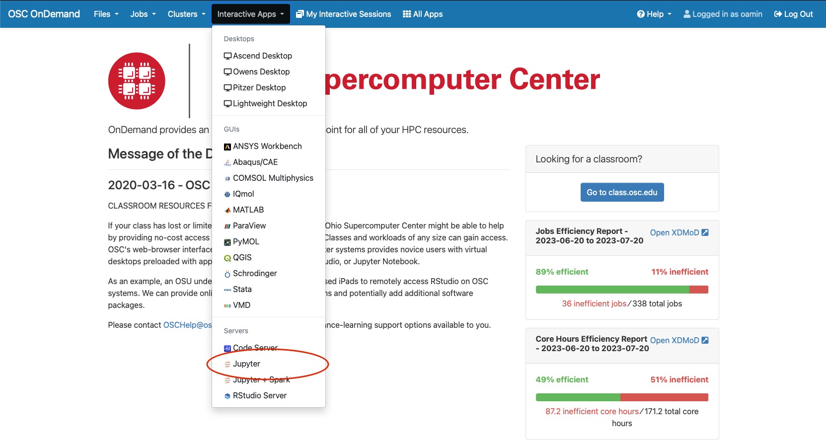
Provide job submission parameters then click Launch.
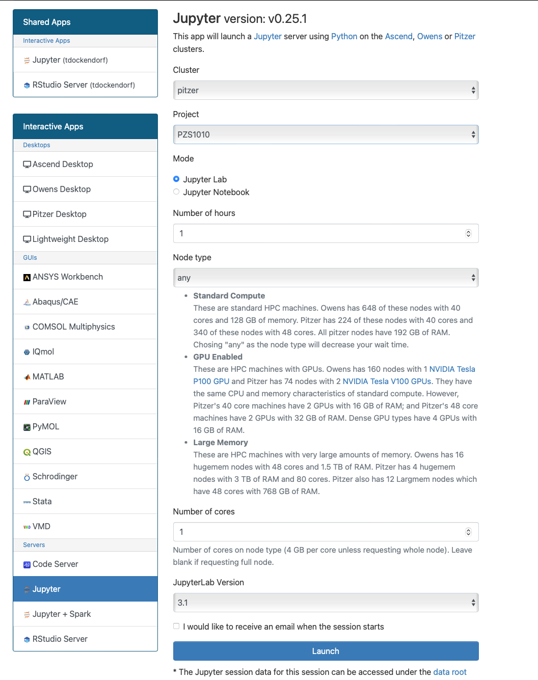
The next page shows the status of your job either as Queued or Starting or Running. Your job may sit in a queue for a few minutes depending on cluster load and resources requested.
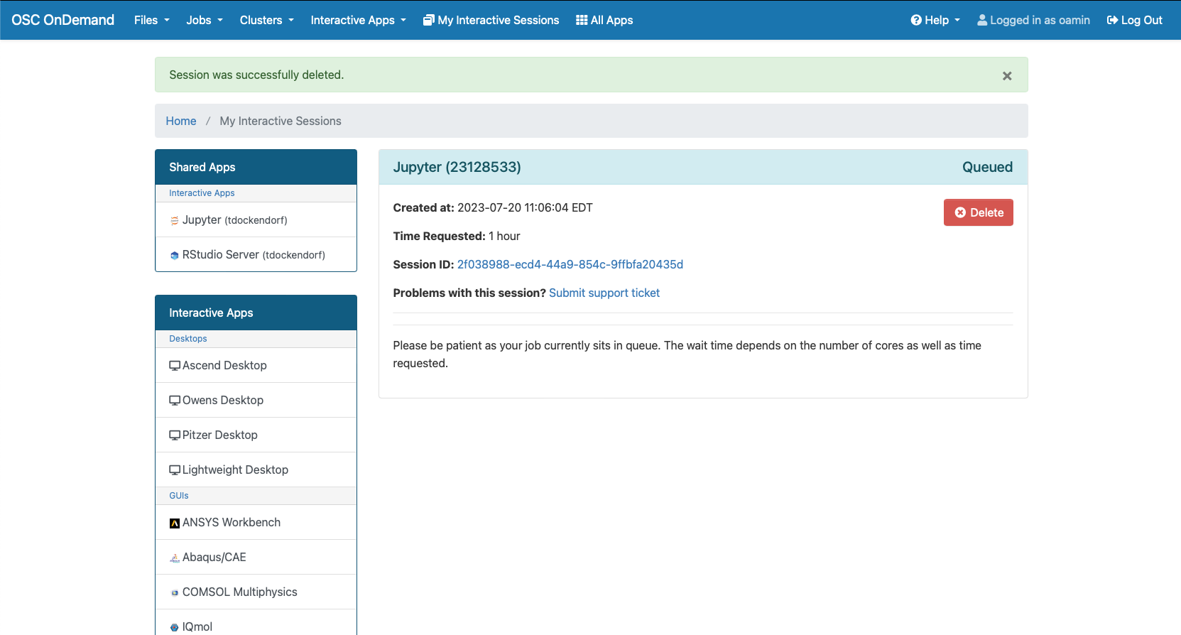
When the job is ready, please click on Connect to Jupyter. This will now launch a Jupyter App.
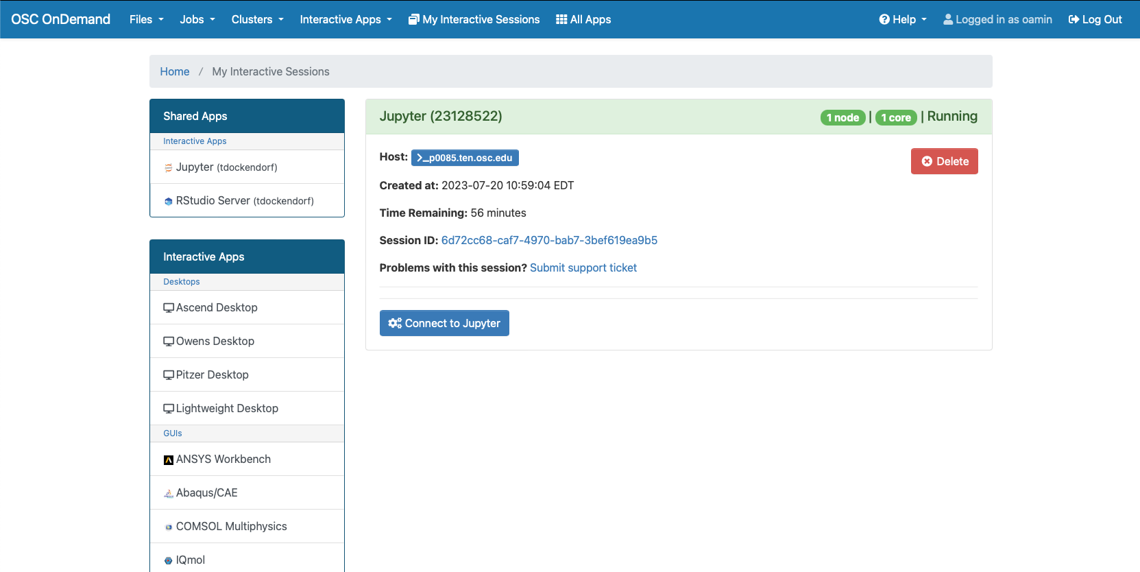
Jupyter App Usage
With the app open, you will be able to access your home directory on the left and all your available kernels will appear on the right. Any custom kernels created using HOWTO: create virtual environment with jupyter will also appear in this selection.
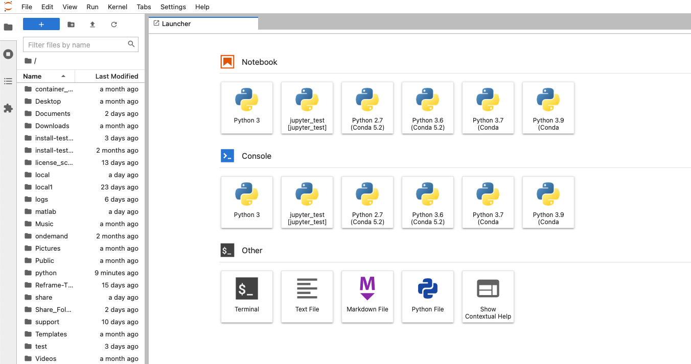
With a file open you can easily switch between different kernels by clicking the kernel name in the top right.
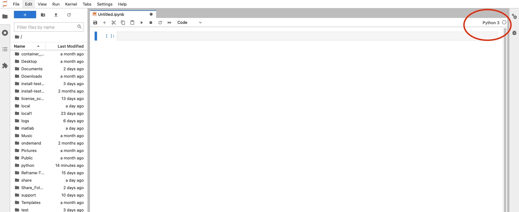
HOW-TOs
Manage your Python packages
We highly recommend creating a local environment using Miniconda3 modules to manage Python packages for your production and research tasks. Please refer to the following how-to pages for more details:
- Create a Local Python Environment
- Install Python Packages from source
- Use Local Python Environment with Jupyter
Install packages for deep/machine learning
Advanced topics
- Use GPU for Python
- Run Python in Parallel
- Python for Classroom (Intended for PI accounts, not for general users)
Known Issues
Incorrect MPI launcher and compiler wrappers with Conda environments
Updated: March 2020
Versions Affected: Python 2.7, 3.6 & Conda 5.2
Versions Affected: Python 2.7, 3.6 & Conda 5.2
Users may encounter under-performing MPI jobs or failures of compiling MPI applications if you are using Conda from system. We found pre-installed mpich2 package in some Conda environments overrides default MPI path. The affected Conda packages are
python/2.7-conda5.2 and python/3.6-conda5.2. If users experience these issues, please re-load MPI module, e.g. module load mvapich2 after setting up your Conda environment.Further reading
Extensive documentation of the Python programming language and software downloads can be found at the Official Python Website.
See Also
Service:
Fields of Science:
Q-Chem
Q-Chem is a general purpose ab initio electronic structure program. Its latest version emphasizes Self-Consistent Field, especially Density Functional Theory, post Hartree-Fock, and innovative algorithms for fast performance and reduced scaling calculations. Geometry optimizations, vibrational frequencies, thermodynamic properties, and solution modeling are available. It performs reasonably well within its single reference paradigm on open shell and excited state systems. The Q-Chem Home Page has additional information.
Availability and Restrictions
Versions
Q-Chem is available on the OSC clusters. These are the versions currently available:
| Version | Owens | Pitzer | Notes |
|---|---|---|---|
| 6.1.0 | X* | X* |
* Current default version
** Starting from version 5.2, a flag '-mpi' is requied for running a MPI job, e.g. qchem -mpi -np 2. Without the flag, OpenMP is the default parallelization.
** Starting from version 5.2, a flag '-mpi' is requied for running a MPI job, e.g. qchem -mpi -np 2. Without the flag, OpenMP is the default parallelization.
On October 12, 2023, we removed all previous versions of QChem, including 4.x, 5.x, and 6.0.x.Therefore, only qchem/6.1.0 is available. This is because of the academic license held by OSC, which permits only the usage of the latest available version. We recommend updating your job scripts if you currently use older versions of QChem: you can use either "module load qchem" or "module load qchem/6.1.0" in your script. Please be aware that moving forward, when a new version becomes available and is installed on OSC, the previous version will also be automatically removed. You can use
module avail qchem to view available modules for a given machine. Feel free to contact OSC Help if you have any questions.Access
Q-chem is available to academic OSC users only. Please review the Q-Chem license agreement carefully before use. If you have any questions, please contact OSC Help.
Publisher/Vendor/Repository and License Type
Q-Chem, Inc., Commercial
Usage
For MPI jobs that request multiple nodes the qchem script must be run from a globally accessible working directory, e.g., project or home directories
Starting with 5.1, QCSCRATCH is automatically set to $TMPDIR which is removed upon the job is completed. This is for saving scratch space and better job performance. If you need to save Q-Chem scratch files from a job and use them later, set QCSCRATCH to globally accessible working directory and QCLOCALSCR to $TMPDIR.
Usage on Owens
Set-up on Owens
Q-Chem usage is controlled via modules. Load one of the Q-Chem modulefiles at the command line, in your shell initialization script, or in your batch scripts. To load the default version of Q-Chem module, usemodule load qchem. To select a particular software version, use module load qchem/version. For example, use module load qchem/4.4.1 to load Q-Chem version 4.4.1 on Owens.
Examples
- The root of the Q-Chem directory tree is /usr/local/qchem/
- Example Q-Chem input files are in the samples subdirectory
Batch Usage on Owens
When you log into owens.osc.edu you are actually logged into a linux box referred to as the login node. To gain access to the mutiple processors in the computing environment, you must submit your job to the batch system for execution. Batch jobs can request mutiple nodes/cores and compute time up to the limits of the OSC systems. Refer to Queues and Reservations and Batch Limit Rules for more info. Batch jobs run on the compute nodes of the system and not on the login node. It is desirable for big problems since more resources can be used.
Interactive Batch Session
For an interactive batch session one can run the following command:
sinteractive -A <project-account> -N 1 -n 1 -t 00:20:00
which requests one core (-N 1 -n 1), for a walltime of 20 minutes (-t 00:20:00). You may adjust the numbers per your need.
Usage on Pitzer
Set-up on Pitzer
Q-Chem usage is controlled via modules. Load one of the Q-Chem modulefiles at the command line, in your shell initialization script, or in your batch scripts. To load the default version of Q-Chem module, usemodule load qchem.
Examples
- The root of the Q-Chem directory tree is /apps/qchem/
- Example Q-Chem input files are in the samples subdirectory
Batch Usage on Pitzer
When you log into pitzer.osc.edu you are actually logged into a linux box referred to as the login node. To gain access to the mutiple processors in the computing environment, you must submit your job to the batch system for execution. Batch jobs can request mutiple nodes/cores and compute time up to the limits of the OSC systems. Refer to Queues and Reservations and Batch Limit Rules for more info. Batch jobs run on the compute nodes of the system and not on the login node. It is desirable for big problems since more resources can be used.
Interactive Batch Session
For an interactive batch session one can run the following command:
sinteractive -A <project-account> -N 1 -n 1 -t 00:20:00
which requests one node (-N 1) and one core (-n 1), for a walltime of 20 minutes (-t 00:20:00). You may adjust the numbers per your need.
Further Reading
Service:
Fields of Science:
QGIS
QGIS is a user friendly Open Source Geographic Information System (GIS) licensed under the GNU General Public License. QGIS is an official project of the Open Source Geospatial Foundation (OSGeo). It runs on Linux, Unix, Mac OSX, Windows and Android and supports numerous vector, raster, and database formats and functionalities.
Availability and Restrictions
Versions
The following versions of QGIS are available on OSC clusters:
| Version | Owens | Pitzer | Note | |
|---|---|---|---|---|
| 3.4.12 | X | X | ||
| 3.6.14 | X | X | ||
| 3.22.1 | X* | X* | ||
| 3.22.8 | X | X | SAGA 7.9.1 available |
* Current default version
Access
QGIS is available to all OSC users via OnDemand QGIS app. If you have any questions, please contact OSC Help.
Publisher/Vendor/Repository and License Type
GNU General Public License.
Further Reading
Service:
Fields of Science:
Quantum Espresso
Quantum ESPRESSO (QE) is a program package for ab-initio molecular dynamics (MD) simulations and electronic structure calculations. It is based on density-functional theory, plane waves, and pseudopotentials.
Availability and Restrictions
Versions
The following versions are available on OSC systems:
| Version | Owens | Pitzer | Note |
|---|---|---|---|
| 5.2.1 | X | ||
| 6.1 | X | ||
| 6.2.1 | X | ||
| 6.3 | X | X | |
| 6.5 | X* | X* | |
| 6.7 | X | X | thermo_pw 1.5 available |
* Current default version
You can use module spider espresso to view available modules for a given machine. Feel free to contact OSC Help if you need other versions for your work.
Access
Quantum ESPRESSO is open source and available to all OSC users. We recommend that Owens be used. If you have any questions, please contact OSC Help.
Publisher/Vendor/Repository and License Type
http://www.quantum-espresso.org, Open source
Usage
Set-up
You can configure your environment for the usage of Quantum ESPRESSO by running the following command:
module load espresso
For QE 6.2.1 and previous versions on Owens, you need to load au2016 by module load modules/au2016 before you load espresso.
In the case of multiple compiled versions load the appropriate compiler first, e.g., on Owens to select the most recently compiled QE 6.1 version use the following commands:
module load intel/17.0.2 module load espresso/6.1
Batch Usage
Sample batch scripts and input files are available here:
~srb/workshops/compchem/espresso/
Further Reading
See Also
Service:
Fields of Science:
R and Rstudio
R is a language and environment for statistical computing and graphics. It is an integrated suite of software facilities for data manipulation, calculation, and graphical display. It includes
- an effective data handling and storage facility,
- a suite of operators for calculations on arrays, in particular matrices,
- a large, coherent, integrated collection of intermediate tools for data analysis,
- graphical facilities for data analysis and display either on-screen or on hardcopy, and
- a well-developed, simple and effective programming language which includes conditionals, loops, user-defined recursive functions and input, and output facilities
More information can be found here.
- Availability and Restrictions
- Usage
- HOWTO: Install Local R Packages
- R packages with external dependencies
- renv: Package Manager
- Parallel R
- R batchtools
- Profiling R code
- Rstudio for classroom
- Troubleshooting issues
Availability and Restrictions
Versions
The following versions of R are available on OSC systems:
| Version | Owens | Pitzer | Ascend |
|---|---|---|---|
| 3.3.2 | X | ||
| 3.4.0 | X | ||
| 3.4.2 | X | ||
| 3.5.0# | X* | ||
| 3.5.1 | X | X* | |
| 3.5.2 | X | ||
| 3.6.0 or 3.6.0-gnu7.3 | X | X | |
| 3.6.1 or 3.6.1-gnu9.1 | X | ||
| 3.6.3 or 3.6.3-gnu9.1 | X | X | |
| 4.0.2 or 4.0.2-gnu9.1 | X | X | |
| 4.1.0 or 4.1.0-gnu9.1** | X | X | |
| 4.2.1 or 4.2.1-gnu11.2 | X | X | X* |
| 4.3.0 or 4.3.0-gnu11.2 | X | X | X |
* Current default version # R/3.5.0 is available for both intel/16 and intel/18, but they may differ for R packages under them. R/3.6.0 and later versions are compiled with gnu and mkl. Loading R/3.6.X modules require dependencies to be preloaded whereas R/3.6.X-gnuY modules will automatically load required dependencies.
** The user state directory (session data) is stored at ~/.local/share/rstudio for the latest RStudio that we have deployed with R/4.1.0. It is located at ~/.rstudio for older versions. Users would need to delete session data from ~/.local/share/rstudio for R/4.1.0 and ~/.rstudio for older versions to clear workspace history.
Known Issue
There's a known issue loading modules in RStudio's environment after changing versions or clusters.
If you have issues using modules in the RConsole - try these remedies
- restarting the terminal
- restarting the RConole
- logging out of the RStudio session and logging back in.
- remove your ~/.local/share/rstudio
You can use module avail R to view available modules and module spider R/version to show how to load the module for a given machine. Feel free to contact OSC Help if you need other versions for your work.
Access
R is available to all OSC users. If you have any questions, please contact OSC Help.
Publisher/Vendor/Repository and License Type
R Foundation, Open source
Usage
R software can be launched two different ways; through Rstudio on OSC OnDemand and through the terminal.
Rstudio
In order to access Rstudio and OSC R workshop materials, please visit here.
Terminal Acess
In order to configure your environment for R, run the following command:
module load R/version #for example, module load R/3.6.3-gnu9.1
R/3.6.0 and onwards versions use gnu compiler and intel mkl libraries for performance improvements. Loading R/3.6.X modules require dependencies to be preloaded as below whereas R/3.6.X-gnuY modules will automatically load required dependencies.
Using R
Once your environment is configured, R can be started simply by entering the following command:
R
For a listing of command line options, run:
R --help
Running R interactively on a login node for extended computations is not recommended and may violate OSC usage policy. Users can either request compute nodes to run R interactively or run R in batch.
Running R interactively on terminal:
Request compute node or nodes if running parallel R as,
sinteractive -A <project-account> -N 1 -n 28 -t 01:00:00
When the compute node is ready, launch R by loading modules
module load R/3.6.3-gnu9.1 R
Batch Usage
Reference the example batch script below. This script requests one full node on the Owens cluster for 1 hour of wall time.
#!/bin/bash
#SBATCH --job-name R_ExampleJob
#SBATCH --nodes=1 --ntasks-per-node=48
#SBATCH --time=01:00:00
#SBATCH --account <your_project_id>
module load R/3.6.3-gnu9.1
cp in.dat test.R $TMPDIR
cd $TMPDIR
R CMD BATCH test.R test.Rout
cp test.Rout $SLURM_SUBMIT_DIR
HOWTO: Install Local R Packages
R comes with a single library $R_HOME/library which contains the standard and recommended packages. This is usually in a system location. On Owens, it is /usr/local/R/gnu/9.1/3.6.3/lib64/R for R/3.6.3. OSC also installs popular R packages into the site located at /usr/local/R/gnu/9.1/3.6.3/site/pkgs for R/3.6.3 on Owens.
Users can check the library path as follows after launching an R session;
> .libPaths() [1] "/users/PZS0680/soottikkal/R/x86_64-pc-linux-gnu-library/3.6" [2] "/usr/local/R/gnu/9.1/3.6.3/site/pkgs" [3] "/usr/local/R/gnu/9.1/3.6.3/lib64/R/library"
Users can check the list of available packages as follows;
>installed.packages()
To install local R packages, use install.package() command. For example,
>install.packages("lattice")
For the first time local installation, it will give a warning as follows:
Installing package into ‘/usr/local/R/gnu/9.1/3.6.3/site/pkgs’
(as ‘lib’ is unspecified)
Warning in install.packages("lattice") :
'lib = "/usr/local/R/gnu/9.1/3.6.3/site/pkgs"' is not writable
Would you like to use a personal library instead? (yes/No/cancel)
Answer y , and it will create the directory and install the package there.
If you are using R older than 3.6, and if you have errors similar to
/opt/intel/18.0.3/compilers_and_libraries_2018.3.222/linux/compiler/include/complex(310): error #308: member "std::complex::_M_value" (declared at line 1346 of "/apps/gnu/7.3.0/include/c++/7.3.0/complex") is inaccessible return __x / __y._M_value;
then create a Makevars file in your project path and add the following command to it:
CXXFLAGS = -diag-disable 308
Set the R_MAKEVARS_USER to the custom Makevars created under your project path as follows
export R_MAKEVARS_USER="/your_project_path/Makevars"
Installing Packages from GitHub
Users can install R packages directly from Github using devtools package as follows
>install.packages("devtools")
>devtools::install_github("author/package")
Installing Packages from Bioconductor
Users can install R packages directly from Bioconductor using BiocManager.
>install.packages("BiocManager")
>BiocManager::install(c("GenomicRanges", "Organism.dplyr"))
R packages with external dependencies
When installing R packages with external dependencies, users may need to import appropriate libraries into R. Sometimes using a gnu version of R can alleviate problems, e.g., try R/4.3.0-gnu11.2 if R/4.3.0 fails. One of the frequently requested R packages is sf which needs geos, gdal and PROJ libraries. We have a few versions of those packages installed and they can be loaded as modules. Another relativey common external dependency is gsl use, e.g.: module spider gsl, to find the available versions of such dependencies.
Here is an example of how to install R package sf.
module load geos/3.9.1 proj/8.1.0 gdal/3.3.1
module load R/4.0.2-gnu9.1
R
>install.packages("sf")
Now you can install other packages that depend on sf normally. Please note that if you get an error indicating the sqlite version is outdated, you can load its module along with geos, proj and gdal modules: module load sqlite/3.26.0
This is an example of the stars package installation, which has a dependency of sf package.
>install.packages("stars")
>library(stars)
When modules of external libs are not available, users can install those and link libraries to the R environment. Here is an example of how to install the sf package on Owens without modules.
Please note that the library paths will change to
/apps/ on Pitzer instead of /usr/local/ as on Owens.Please note that if you get an error indicating the sqlite version is outdated, you can load its module before proceeding with the installation:
module load sqlite/3.26.0
>old_ld_path <- Sys.getenv("LD_LIBRARY_PATH")
>Sys.setenv(LD_LIBRARY_PATH = paste(old_ld_path, "/usr/local/gdal/3.3.1/lib", "/usr/local/proj/8.1.0/lib","/usr/local/geos/3.9.1/",sep=":"))
>Sys.setenv("PKG_CONFIG_PATH"="/usr/local/proj/8.1.0/lib/pkgconfig")
>Sys.setenv("GDAL_DATA"="/usr/local/gdal/3.3.1/share/gdal")
>install.packages("sf", configure.args=c("--with-gdal-config=/usr/local/gdal/3.3.1/bin/gdal-config","--with-proj-include=/usr/local/proj/8.1.0/include","--with-proj-lib=/usr/local/proj/8.1.0/lib","--with-geos-config=/usr/local/geos/3.9.1/bin/geos-config"),INSTALL_opts="--no-test-load")
>dyn.load("/usr/local/gdal/3.3.1/lib/libgdal.so")
>dyn.load("/usr/local/geos/3.9.1/lib/libgeos_c.so", local=FALSE)
>library(sf)
Please note that every time before loading sf package, you have to execute the dyn.load of both libraries listed above. In addition, the first time you install an external package you should answer yes to using and creating a personal library, e.g.:
'lib = "/usr/local/R/gnu/9.1/4.0.2/site/pkgs"' is not writable. Would you like to use a personal library instead? (yes/No/cancel) yes. Would you like to create a personal library '~/R/x86_64-pc-linux-gnu-library/4.0' to install packages into? (yes/No/cancel) yes.
You can install other packages that depend on sf as follows. This is an example of terra package installation.
>install.packages("terra", configure.args=c("--with-gdal-config=/usr/local/gdal/3.3.1/bin/gdal-config","--with-proj-include=/usr/local/proj/8.1.0/include","--with-proj-lib=/usr/local/proj/8.1.0/lib","--with-geos-config=/usr/local/geos/3.9.1/bin/geos-config"),INSTALL_opts="--no-test-load")
>library(terra)
Import modules in R
Alternatively you can load modules in R for those external depedencies if they are available on system
> source(file.path(Sys.getenv("LMOD_PKG"), "init/R"))
> module("load", "geos")
You can check if an external pacakge is available
> module("avail", "geos")
renv: Package Manager
if you are using R for multiple projects, OSC recommendsrenv, an R dependency manager for R package management. Please see more information here.
The renv package helps you create reproducible environments for your R projects. Use renv to make your R projects more:
-
Isolated: Each project gets its own library of R packages, so you can feel free to upgrade and change package versions in one project without worrying about breaking your other projects.
-
Portable: Because
renvcaptures the state of your R packages within a lockfile, you can more easily share and collaborate on projects with others, and ensure that everyone is working from a common base. -
Reproducible: Use
renv::snapshot()to save the state of your R library to the lockfilerenv.lock. You can later userenv::restore()to restore your R library exactly as specified in the lockfile.
Users can install renv package as follows;
>install.packages("renv")
The core essence of the renv workflow is fairly simple:
-
After launching R, go to your project directory using R command
setwdand initiaterenv:setwd("your/project/path") renv::init()This function forks the state of your default R libraries into a project-local library. A project-local
.Rprofileis created (or amended), which is then used by new R sessions to automatically initializerenvand ensure the project-local library is used.Work in your project as usual, installing and upgrading R packages as required as your project evolves.
-
Use
renv::snapshot()to save the state of your project library. The project state will be serialized into a file calledrenv.lockunder your project path. -
Use
renv::restore()to restore your project library from the state of your previously-created lockfilerenv.lock.
In short: use renv::init() to initialize your project library, and use renv::snapshot() / renv::restore() to save and load the state of your library.
After your project has been initialized, you can work within the project as before, but without fear that installing or upgrading packages could affect other projects on your system.
Global Cache
One of renv’s primary features is the use of a global package cache, which is shared across all projects using renvWhen using renv the packages from various projects are installed to the global cache. The individual project library is instead formed as a directory of symlinks into the renv global package cache. Hence, while each renv project is isolated from other projects on your system, they can still re-use the same installed packages as required. By default, global Cache of renv is located ~/.local/share/renvUser can change the global cache location using RENV_PATHS_CACHE variable. Please see more information here.
Please note that renv does not load packages from site location (add-on packages installed by OSC) to the rsession. Users will have access to the base R packages only when using renv. All other packages required for the project should be installed by the user.
Version Control with renv
If you would like to version control your project, you can utilize git versioning of renv.lock file. First, initiate git for your project directory on a terminal
git init
Continue working on your R project by launching R, installing packages, saving snapshot using renv::snapshot()command. Please note that renv::snapshot() will only save packages that are used in the current project. To capture all packages within the active R libraries in the lockfile, please see the type option.
>renv::snapshot(type="simple")
If you’re using a version control system with your project, then as you call renv::snapshot() and later commit new lockfiles to your repository, you may find it necessary later to recover older versions of your lockfiles. renv provides the functions renv::history()to list previous revisions of your lockfile, and renv::revert() to recover these older lockfiles.
If you are using renvpackage for the first time, it is recommended that you check R startup files in your $HOME such as .Rprofile and .Renviron and remove any project-specific settings from these files. Please also make sure you do not have any project-specific settings in ~/.R/Makevars.
A Simple Example
First, you need to load the module for R and fire up R session
module load R/3.6.3-gnu9.1 R
Then set the working directory and initiate renv
setwd("your/project/path")
renv::init()
Let's install a package called lattice, and save the snapshot to the renv.lock
renv::install("lattice")
renv::snapshot(type="simple")
The latticepackage will be installed in global cache of renv and symlink will be saved in renv under the project path.
Restore a Project
Use renv::restore() to restore a project's dependencies from a lockfile, as previously generated by snapshot(). Let's remove the lattice package.
renv::remove("lattice")
Now let's restore the project from the previously saved snapshot so that the lattice package is restored.
renv::restore() library(lattice)
Collaborating with renv
When using renv, the packages used in your project will be recorded into a lockfile, renv.lock. Because renv.lock records the exact versions of R packages used within a project, if you share that file with your collaborators, they will be able to use renv::restore() to install exactly the same R packages as recorded in the lockfile. Please find more information here.
Parallel R
R provides a number of methods for parallel processing of the code. Multiple cores and nodes available on OSC clusters can be effectively deployed to run many computations in R faster through parallelism.
Consider this example, where we use a function that will generate values sampled from a normal distribution and sum the vector of those results; every call to the function is a separate simulation.
myProc <- function(size=1000000) {
# Load a large vector
vec <- rnorm(size)
# Now sum the vec values
return(sum(vec))
}
Serial execution with loop
Let’s first create a serial version of R code to run myProc() 100x on Owens
tick <- proc.time()
for(i in 1:100) {
myProc()
}
tock <- proc.time() - tick
tock
## user system elapsed
## 6.437 0.199 6.637
Here, we execute each trial sequentially, utilizing only one of our 28 processors on this machine. In order to apply parallelism, we need to create multiple tasks that can be dispatched to different cores. Using apply() family of R function, we can create multiple tasks. We can rewrite the above code to use apply(), which applies a function to each of the members of a list (in this case the trials we want to run):
tick <- proc.time()
result <- lapply(1:100, function(i) myProc())
tock <-proc.time() - tick
tock
## user system elapsed
## 6.346 0.152 6.498
parallel package
The parallellibrary can be used to dispatch tasks to different cores. The parallel::mclapply function can distributes the tasks to multiple processors.
library(parallel)
cores <- system("nproc", intern=TRUE)
tick <- proc.time()
result <- mclapply(1:100, function(i) myProc(), mc.cores=cores)
tock <- proc.time() - tick
tock
## user system elapsed
## 8.653 0.457 0.382
foreach package
The foreach package provides a looping construct for executing R code repeatedly. It uses the sequential %do% operator to indicate an expression to run.
library(foreach)
tick <- proc.time()
result <-foreach(i=1:100) %do% {
myProc()
}
tock <- proc.time() - tick
tock
## user system elapsed
## 6.420 0.018 6.439
doParallel package
foreach supports a parallelizable operator %dopar% from the doParallel package. This allows each iteration through the loop to use different cores.
library(doParallel, quiet = TRUE)
library(foreach)
cl <- makeCluster(28)
registerDoParallel(cl)
tick <- proc.time()
result <- foreach(i=1:100, .combine=c) %dopar% {
myProc()
}
tock <- proc.time() - tick
tock
invisible(stopCluster(cl))
detachDoParallel()
## user system elapsed
## 0.085 0.013 0.446
Rmpi package
Rmpi package allows to parallelize R code across multiple nodes. Rmpi provides an interface necessary to use MPI for parallel computing using R. This allows each iteration through the loop to use different cores on different nodes. Rmpijobs cannot be run with RStudio at OSC currently, instead users can submit Rmpi jobs through terminal App. R uses openmpi as MPI interface therefor users would need to load openmpi module before installing or using Rmpi. Rmpi is installed at central location for R versions prior to 4.2.1. If it is not availbe, users can install it as follows
Rmpi Installation
# Get source code of desired version of RMpi wget https://cran.r-project.org/src/contrib/Rmpi_0.6-9.2.tar.gz # Load modules ml openmpi/1.10.7 R/4.2.1-gnu11.2 # Install RMpi R CMD INSTALL --configure-vars="CPPFLAGS=-I$MPI_HOME/include LDFLAGS='-L$MPI_HOME/lib'" --configure-args="--with-Rmpi-include=$MPI_HOME/include --with-Rmpi-libpath=$MPI_HOME/lib --with-Rmpi-type=OPENMPI" Rmpi_0.6-9.2.tar.gz # Test loading library(Rmpi)
Please make sure that $MPI_HOME is defined after loading openmpi module. Newer versions of openmpi module has $OPENMPI_HOME instead of $MPI_HOME. So you would need to replace $MPI_HOME with $OPENMPI_HOME for those versions of openmpi.
Above example code can be rewritten to utilize multiple nodes with Rmpias follows;
library(Rmpi)
library(snow)
workers <- as.numeric(Sys.getenv(c("PBS_NP")))-1
cl <- makeCluster(workers, type="MPI") # MPI tasks to use
clusterExport(cl, list('myProc'))
tick <- proc.time()
result <- clusterApply(cl, 1:100, function(i) myProc())
write.table(result, file = "foo.csv", sep = ",")
tock <- proc.time() - tick
tock
Batch script for job submission is as follows;
#!/bin/bash
#SBATCH --time=10:00
#SBATCH --nodes=2 --ntasks-per-node=28
#SBATCH --account=<project-account>
module load R/3.6.3-gnu9.1 openmpi/1.10.7
# parallel R: submit job with one MPI master
mpirun -np 1 R --slave < Rmpi.R
pbdMPI package
pbdMPI is an improved version of RMpi package that provides efficient interface to MPI by utilizing S4 classes and methods with a focus on Single Program/Multiple Data ('SPMD') parallel programming style, which is intended for batch parallel execution.
Installation of pbdMPI
Users can download latest version of pbdMPI from CRAN https://cran.r-project.org/web/packages/pbdMPI/index.html and install it as follows,
wget https://cran.r-project.org/src/contrib/pbdMPI_0.4-6.tar.gz ml R/4.3.0-gnu11.2 ml openmpi/4.1.4-hpcx R CMD INSTALL pbdMPI_0.4-6.tar.gz
Examples
Here are few resources that demonstrate how to use pbdMPI
https://citeseerx.ist.psu.edu/viewdoc/download;jsessionid=BD40B7B615DF79...
http://hpcf-files.umbc.edu/research/papers/pbdRtara2013.pdf
R Batchtools
The R package, batchtools provides a parallel implementation of Map for high-performance computing systems managed by schedulers Slurm on OSC system. Please find more info here https://github.com/mllg/batchtools.
Users would need two files slurm.tmpl and .batch.conf.R
Slurm.tmpl is provided below. Please change "your project_ID".
#!/bin/bash -l
## Job Resource Interface Definition
## ntasks [integer(1)]: Number of required tasks,
## Set larger than 1 if you want to further parallelize
## with MPI within your job.
## ncpus [integer(1)]: Number of required cpus per task,
## Set larger than 1 if you want to further parallelize
## with multicore/parallel within each task.
## walltime [integer(1)]: Walltime for this job, in seconds.
## Must be at least 60 seconds.
## memory [integer(1)]: Memory in megabytes for each cpu.
## Must be at least 100 (when I tried lower values my
## jobs did not start at all).
## Default resources can be set in your .batchtools.conf.R by defining the variable
## 'default.resources' as a named list.
<%
# relative paths are not handled well by Slurm
log.file = fs::path_expand(log.file)
-%>
#SBATCH --job-name=<%= job.name %>
#SBATCH --output=<%= log.file %>
#SBATCH --error=<%= log.file %>
#SBATCH --time=<%= ceiling(resources$walltime / 60) %>
#SBATCH --ntasks=1
#SBATCH --cpus-per-task=<%= resources$ncpus %>
#SBATCH --mem-per-cpu=<%= resources$memory %>
#SBATCH --account=your_project_id
<%= if (!is.null(resources$partition)) sprintf(paste0("#SBATCH --partition='", resources$partition, "'")) %>
<%= if (array.jobs) sprintf("#SBATCH --array=1-%i", nrow(jobs)) else "" %>
## Initialize work environment like
## source /etc/profile
## module add ...
module add R/4.0.2-gnu9.1
## Export value of DEBUGME environemnt var to slave
export DEBUGME=<%= Sys.getenv("DEBUGME") %>
<%= sprintf("export OMP_NUM_THREADS=%i", resources$omp.threads) -%>
<%= sprintf("export OPENBLAS_NUM_THREADS=%i", resources$blas.threads) -%>
<%= sprintf("export MKL_NUM_THREADS=%i", resources$blas.threads) -%>
## Run R:
## we merge R output with stdout from SLURM, which gets then logged via --output option
Rscript -e 'batchtools::doJobCollection("<%= uri %>")'
.batch.conf.R is provided below.
cluster.functions = makeClusterFunctionsSlurm(template="path/to/slurm.tmpl")
A test example is provided below. Assuming the current working directory has both slurm.tmpl and .batch.conf.R files.
ml R/4.0.2-gnu9.1
R
>install.packages("batchtools")
>library(batchtools)
>myFct <- function(x) {
result <- cbind(iris[x, 1:4,],
Node=system("hostname", intern=TRUE),
Rversion=paste(R.Version()[6:7], collapse="."))}
>reg <- makeRegistry(file.dir="myregdir", conf.file=".batchtools.conf.R")
>Njobs <- 1:4 # Define number of jobs (here 4)
>ids <- batchMap(fun=myFct, x=Njobs)
>done <- submitJobs(ids, reg=reg, resources=list( walltime=60, ntasks=1, ncpus=1, memory=1024))
>waitForJobs()
>getStatus() # Summarize job
Profiling R code
Profiling R code helps to optimize the code by identifying bottlenecks and improve its performance. There are a number of tools that can be used to profile R code.
Grafana:
OSC jobs can be monitored for CPU and memory usage using grafana. If your job is in running status, you can get grafana metrics as follows. After log in to OSC OnDemand, select Jobs from the top tabs, then select Active Jobs and then Job that you are interested to profile. You will see grafana metrics at the bottom of the page and you can click on detailed metrics to access more information about your job at grafana.
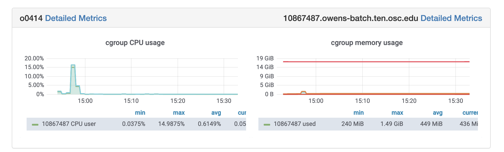
Rprof:
R’s built-in tool,Rprof function can be used to profile R expressions and the summaryRprof function to summarize the result. More information can be found here.
Here is an example of profiling R code with Rprofe for data analysis on Faithful data.
Rprof("Rprof-out.prof",memory.profiling=TRUE, line.profiling=TRUE)
data(faithful)
summary(faithful)
plot(faithful)
Rprof(NULL)
To analyze profiled data, runsummaryRprof on Rprof-out.prof
summaryRprof("Rprof-out.prof")
You can read more about summaryRprofhere.
Profvis:
It provides an interactive graphical interface for visualizing data from Rprof.
library(profvis)
profvis({
data(faithful)
summary(faithful)
plot(faithful)
},prof_output="profvis-out.prof")
If you are running the R code on Rstudio, it will automatically open up the visualization for the profiled data. More info can be found here.
Using Rstudio for classroom
OSC provides an isolated and custom R environment for each classroom project that requires Rstudio. More information can be found here.
Further Reading
Troubleshooting issues
1. If you're encountering difficulties launching the RStudio App on-demand, it's recommended to review your ~/.bashrc file for any conda/python configurations. Consider commenting out these configurations and attempting to launch the app again.
2. If your R session is taking too long to initialize, it might be due to issues from a previous session. To resolve this, consider restoring R to a fresh session by removing the previous state stored at
~/.local/share/rstudio (~/.rstudio for <R/4.1)
mv ~/.local/share/rstudio ~/.local/share/rstudio.backup
Further Reading
See Also
Service:
Fields of Science:
RELION
RELION (REgularised LIkelihood OptimisatioN) is a stand-alone computer program for the refinement of 3D reconstructions or 2D class averages in electron cryo-microscopy.
We have identified some issues with the RELION installations. For more details, please refere the "Known Issues" section below.
To address the issues, we have decided to deprecate affected versions, including: relion/3.1, relion/3.1-gpu, relion/3.1.3, relion/4.0.0, and relion/4.0b on both Owens and Pitzer. Additionally, we will deprecate other versions that are rarely used to improve maintenance. These versions include relion2/2.0 and relion/3.0.4.
The deprecation action was done on January 23, 2024. To migrate your jobs, please refer to the "Versions" table below for available versions. If you require any assistance, please contact OSC help.
Availability and Restrictions
Versions
RELION is available on the Owens cluster. The versions currently available at OSC are:
| Version | Owens | Pitzer | Ascend | Note |
|---|---|---|---|---|
| 3.1-cuda10.1 | X | Built with CUDA 10.1 | ||
| 4.0-cuda10.1 | X | RELION 4.0 beta2 Built with CUDA 10.1 |
||
| 4.0.1 | X | X | X | Built with CUDA 10.2 (11.8 for Ascend) |
| 5.0b | X | Built with CUDA 11.8 |
* Current Default Version
You can use module spider relion to view available modules for a given machine. Feel free to contact OSC Help if you need other versions for your work.
Available third-party packages
| Cluster | RELION | CTFFIND | MotionCor2 | GCTF | ResMap | Unblur & Summovie |
|---|---|---|---|---|---|---|
| Pitzer | 4.0.1, 5.0b | 4.1.14 | 1.4.4 | 1.18 | 1.1.4 | 1.0.2 |
| Ascend | 4.0.1 | 4.1.14 | 1.4.5 | 1.18 | 1.1.4 | 1.0.2 |
Access
RELION is available to all OSC users.
Publisher/Vendor/Repository and License Type
MRC Lab of Molecular Biology, Open source
Usage
Usage on Owens
Set-up
To set up the environment for RELION on the Owens cluster, use the command:
module load relion/version
where version is chosen from the available versions (omitting the version will load the default version).
Usage on Pitzer
Set-up
To set up the environment for RELION on the Pitzer cluster, use the command:
module load relion/version
where version is chosen from the available versions (omitting the version will load the default version).
Known issues
Hybrid MPI+OpenMP job Hangs on multiple nodes
Update: January 2024
Version: All Intel+MVAPICH2 versions
Version: All Intel+MVAPICH2 versions
Hybrid MPI+OpenMP jobs utilizing programs built with the Intel compiler and MVAPICH2 may experience hangs when running on multiple nodes. This issue is attributed to a known problem in MVAPICH2 built with the Intel compiler stack.
Resolution
All versions of Intel+MVAPICH2 have been removed to address this issue.
Poor performance with hybrid MPI+OpenMPI jobs and more than 4 MPI Tasks on multiple nodes
Update: January 2024
Version: Prior to 5
Version: Prior to 5
RELION versions prior to 5 may exhibit poor performance in hybrid MPI+OpenMP jobs when the number of MPI tasks exceeds 4 on multiple nodes.
Resolution
If possible, limit the number of MPI tasks to 4 or less for optimal performance. Consider using RELION version 5 or later, as newer versions may include optimizations and improvements that address this performance issue.
Further Reading
RNA-SeQC
RNA-SeQC is a java program which computes a series of quality control metrics for RNA-seq data. The input can be one or more BAM files. The output consists of HTML reports and tab delimited files of metrics data. This program can be valuable for comparing sequencing quality across different samples or experiments to evaluate different experimental parameters. It can also be run on individual samples as a means of quality control before continuing with downstream analysis.
Availability and Restrictions
Versions
The following versions of RNA-SeQC are available on OSC clusters:
| Version | Owens |
|---|---|
| 1.1.8 | X* |
* Current default version
You can use module spider rna-seqc to view available modules for a given machine. Feel free to contact OSC Help if you need other versions for your work.
Access
RNA-SeQC is available to all OSC users. If you have any questions, please contact OSC Help.
Publisher/Vendor/Repository and License Type
The Broad Insitute, Open source
Usage
Usage on Owens
Set-up
To configure your environment for use of RNA-SeQC, run the following command:
module load rna-seqc. The default version will be loaded. To select a particular RNA-SeQC version, use module load rna-seqc/version. For example, use module load rna-seqc/1.1.8 to load RNA-SeQC 1.1.8.Usage
This software is a Java executable .jar file; thus, it is not possible to add to the PATH environment variable.
From module load rna-seqc, a new environment variable, RNA_SEQC, will be set. Thus, users can use the software by running the following command: java -jar $RNA_SEQC {other options}.
Further Reading
Supercomputer:
Service:
Fields of Science:
Rosetta
Rosetta is a software suite that includes algorithms for computational modeling and analysis of protein structures. It has enabled notable scientific advances in computational biology, including de novo protein design, enzyme design, ligand docking, and structure prediction of biological macromolecules and macromolecular complexes.
Availability and Restrictions
Versions
The Rosetta suite is available on Owens and Pitzer. The versions currently available at OSC are:
| Version | Owens | Pitzer |
|---|---|---|
| 3.10 | X | X |
| 3.12 | X* | X* |
* Current default version
You can use module spider rosetta to view available modules for a given machine. Feel free to contact OSC Help if you need other versions for your work.
Access for Academic Users
Rosetta is available to academic OSC users. Please review the license agreement carefully before use. If you have any questions, please contact OSC Help.
Publisher/Vendor/Repository and License Type
Rosetta, Non-Commercial
Usage
Usage on Owens and Pitzer
To set up your environment for rosetta load one of its module files:
module load rosetta/3.12
Here is an example batch script that uses Rosetta Abinitio Relax application:
#!/bin/bash
#SBATCH --job-name="rosetta_abinitio_relax_job"
#SBATCH --ntasks=1
#SBATCH --time=0:10:0
#SBATCH --account=PAS1234
scontrol show job $SLURM_JOB_ID
export
module reset
module load rosetta/3.12
module list
echo $TMPDIR
cd $TMPDIR
mkdir input_files
sbcast -p $ROSETTA3/demos/tutorials/denovo_structure_prediction/Denovo_structure_prediction.md $TMPDIR/Denovo_structure_prediction.md
sbcast -p $ROSETTA3/demos/tutorials/denovo_structure_prediction/folding_funnels.png $TMPDIR/folding_funnels.png
cd $ROSETTA3/demos/tutorials/denovo_structure_prediction/input_files/
for FILE in *
do
sbcast -p $FILE $TMPDIR/input_files/$FILE
done
cd $TMPDIR
AbinitioRelax.linuxiccrelease @input_files/options
ls -l
sgather -pr $TMPDIR ${SLURM_SUBMIT_DIR}/sgather
Here is an example batch script that uses Rosetta MPI Docking script:
#!/bin/bash
#SBATCH --job-name="rosetta_scripts_mpi_docking_job"
#SBATCH --nodes=2
#SBATCH --time=0:10:0
#SBATCH --account=PAS1234
scontrol show job $SLURM_JOB_ID
export
module reset
module load rosetta/3.12
module list
sbcast -p ~support/share/reframe/source/rosetta/6shs_PIB.pdb $TMPDIR/6shs_PIB.pdb
sbcast -p ~support/share/reframe/source/rosetta/pib-abeta.xml $TMPDIR/pib-abeta.xml
sbcast -p ~support/share/reframe/source/rosetta/pib.params $TMPDIR/pib.params
cd $TMPDIR
srun rosetta_scripts.mpi -s 6shs_PIB.pdb -nstruct 100 -extra_res_fa pib.params -parser:protocol pib-abeta.xml -add_orbitals True -out:prefix t_ -out:pdb True
sgather -pr $TMPDIR ${SLURM_SUBMIT_DIR}/sgather
Further Reading
Supercomputer:
Service:
Fields of Science:
SAMtools
SAM format is a generic format for storing large nucleotide sequence alignments. SAMtools provide various utilities for manipulating alignments in the SAM format, including sorting, merging, indexing and generating alignments in a per-position format.
Availability and Restrictions
The following versions of SAMtools are available on OSC clusters:
| Version | Owens | Pitzer |
|---|---|---|
| 1.3.1 | X | |
| 1.6 | X | |
| 1.8 | X | |
| 1.9 | X | |
| 1.10 | X* | X* |
| 1.16.1 | X | X |
* Current default version
You can use module spider samtools to view available modules for a given machine. Feel free to contact OSC Help if you need other versions for your work.
Access
SAMtools is available to all OSC users. If you have any questions, please contact OSC Help.
Publisher/Vendor/Repository and License Type
Genome Research Ltd., Open source
Usage
Usage on Owens
Set-up
To configure your environment for use of SAMtools, run the following command:
module load samtools . The default version will be loaded. To select a particular SAMtools version, use module load samtools/version . For example, use module load samtools/1.3.1 to load SAMtools 1.3.1.Usage on Pitzer
Set-up
To configure your environment for use of SAMtools, run the following command:
module load samtools . The default version will be loaded. Further Reading
Service:
Fields of Science:
SIESTA
SIESTA is both a method and its computer program implementation, to perform efficient electronic structure calculations and ab initio molecular dynamics simulations of molecules and solids. More information can be found from here.
Availability and Restrictions
Versions
SIESTA is available on the Owens and Oakley clusters. A serial and a parallel build were created in order to meet users' computational needs.
| Version | Owens | Pitzer |
|---|---|---|
| 4.0 | X | |
| 4.0.2 | X* | X* |
* Current default version
You can use module spider siesta to view available modules for a given machine. Feel free to contact OSC Help if you need other versions for your work.
Access
SIESTA newer than version 4.0 is under GPL license. Therefore, any users can access SIESTA on Owens. If you have any questions, please contact OSC Help for further information.
Publisher/Vendor/Repository and License Type
https://departments.icmab.es/leem/siesta/, Open source
Usage
Batch Usage
When you log into oakley.osc.edu or owens.osc.edu, you are actually logged into a linux box referred to as the login node. To gain access to the 4000+ processors in the computing environment, you must submit your SIESTA job to the batch system for execution.
Assume that you have a test case in your work directory (where you submit your job, represented by $PBS_O_WORKDIR), with the input file 32_h2o.fdf. A batch script can be created and submitted for a serial or parallel run. The following are the sample batch scripts for running serial and parallel SIESTA jobs. Sample batch scripts and input files are also available here:
~srb/workshops/compchem/siesta/
Sample Batch Script for Serial Jobs
#!/bin/bash #SBATCH --time=0:30:00 #SBATCH --nodes=1 --ntasks-per-node=28 #SBATCH --job-name=siesta #SBATCH --account <project-account> # # Set up the package environment module load siesta # # Execute the serial solver (nodes=1, ppn<=12) siesta <32_h2o.fdf> output exit
NOTE: Change ntasks-per-node to = 28 for Owens
Sample Batch Script for Parallel Jobs
#!/bin/bash #SBATCH --time=0:30:00 #SBATCH --nodes=2 --ntasks-per-node=28 #SBATCH --job-name=siesta #SBATCH --account <project-account> # # Set up the package environment module swap intel/12.1.4.319 intel/13.1.3.192 module load siesta_par # # Execute the parallel solver (nodes>1, ppn=28) srun siesta <32_h2o.fdf> output exit
NOTE: Change ntasks-per-node to = 28 for Owens
Usage on Pitzer
#!/bin/bash #SBATCH --time=0:30:00 #SBATCH --nodes=1 --ntasks-per-node=48 #SBATCH --job-name=siesta #SBATCH --account <project-account> # # Set up the package environment module load siesta # # Execute the serial solver (nodes=1, ppn<=48) siesta <32_h2o.fdf> output exit
Further Reading
Online documentation is available at the SIESTA homepage.
Citations
This is required for the versions older than 4.0.
1. “Self-consistent order-N density-functional calculations for very large systems”, P. Ordejón, E. Artacho and J. M. Soler, Phys. Rev. B (Rapid Comm.) 53, R10441-10443 (1996).
2. “The SIESTA method for ab initio order-N materials simulation”, J. M. Soler, E. Artacho,J. D. Gale, A. García, J. Junquera, P. Ordejón, and D. Sánchez-Portal, J. Phys.: Condens. Matt. 14, 2745-2779 (2002).
Service:
SRA Toolkit
The Sequence Read Archive (SRA Toolkit) stores raw sequence data from "next-generation" sequencing technologies including 454, IonTorrent, Illumina, SOLiD, Helicos and Complete Genomics. In addition to raw sequence data, SRA now stores alignment information in the form of read placements on a reference sequence. Use SRA Toolkit tools to directly operate on SRA runs.
Availability and Restrictions
The following versions of SRA Toolkit are available on OSC clusters:
| Version | Owens | Pitzer | Note |
|---|---|---|---|
| 2.6.3 | X | These versions no longer support downloading SRA data** but still can be used to process local data. | |
| 2.9.0 | X | ||
| 2.9.1 | X | ||
| 2.9.6 | X* | X* | |
| 2.10.7 | X | X | |
| 2.11.2 | X | X | |
| 3.0.2 | X | X |
* Current default version
** NCBI now uses cloud-style object stores. To access SRA cloud data, use version 2.10 or later and provide your AWS or GCP access credentials (recommended) to vdb-config. For more information, see https://github.com/ncbi/sra-tools/wiki/04.-Cloud-Credentials.
You can use module spider sratoolkit to view available modules for a given machine. Feel free to contact OSC Help if you need other versions for your work.
Access
SRA Toolkit is available to all OSC users. If you have any questions, please contact OSC Help.
Publisher/Vendor/Repository and License Type
National Center for Biotechnology Information, Freeware
Usage
Usage on Pitzer and Owens
Set-up
To configure your environment for use of SRA Toolkit, run the following command:
module load sratoolkit. The default version will be loaded. To select a particular SRA Toolkit version, use module load sratoolkit/version. For example, use module load sratoolkit/2.11.2 to load SRA Toolkit 2.11.2Download SRA Data
NCBI now uses cloud-style object stores. To access SRA cloud data, use version 2.10 or later and provide your AWS or GCP access credentials (recommended) to vdb-config. For more information, see https://github.com/ncbi/sra-tools/wiki/04.-Cloud-Credentials.
Set up the credentials (recommended)
Once you have obtained an AWS or GCP credential file, you can set the credentials by following these steps:
module load sratoolkit/2.11.2 vdb-config --report-cloud-identity yes # For GCP credentials vdb-config --set-gcp-credentials /path/to/gcp/creddential/file # For AWS credentials vdb-config --set-aws-credentials /path/to/aws/creddential/file
Each version of the toolkit comes with its own set of configuration options. To modify the defaults, run
vdb-config -i to access the interactive configuration. For additional information, please visit the following link: https://github.com/ncbi/sra-tools/wiki/03.-Quick-Toolkit-Configuration.You can now download SRA data using prefetch
prefetch SRR390728
The default download path is located in your home directory at ~/ncbi. For instance, if you're looking for the SRA file SRR390728.sra, you can find it at ~/ncbi/sra, and the resource files can be found at ~/ncbi/refseq. You can use srapath to verify if the SRA accession is accessible in the download path
$ srapath SRR390728
/users/PAS1234/johndoe/ncbi/sra/sra/SRR390728.sra
You can now run other SRA tools, such as fastq-dump, on computing nodes. Here is an example job script:
#!/bin/bash #SBATCH --job-name use_fastq_dump #SBATCH --time=0:10:0 #SBATCH --ntask=1 module load sratoolkit/2.11.2 module list fastq-dump -X 5 -Z SRR390728
Unfortunately, Home Directory file system is not optimized for handling heavy computations. If the SRA file is particularly large, you can change the default download path for SRA data to our scratch file system using one of the following two approaches. The following approaches use the /fs/scratch/PAS1234/johndoe/ncbi directory as an example.
Change the prefetch directory using vdb-config
module load sratoolkit/2.11.2 vdb-config -s /repository/user/main/public/root=/fs/scratch/PAS1234/johndoe/ncbi prefetch SRR390728 srapath SRR390728
You should find the SRR390728 accession at /fs/scratch/PAS1234/johndoe/ncbi/sra/SRR390728.sra
Download to the current directory (available for version 2.10 or later)
module load sratoolkit/2.11.2
vdb-config --prefetch-to-cwd
mkdir -p /fs/scratch/PAS1234/johndoe/ncbi
cd /fs/scratch/PAS1234/johndoe/ncbi
prefetch SRR390728
srapath SRR390728
You should find the SRR390728 accession at /fs/scratch/PAS1234/johndoe/ncbi/SRR390728/SRR390728.sra
Known Issues
Error when downloading SRA data
NCBI now utilizes cloud-style object stores. To access SRA cloud data, please use version 2.10 or later and provide your AWS or GCP access credentials to vdb-config. For more information, please visit https://github.com/ncbi/sra-tools/wiki/04.-Cloud-Credentials. However, you can continue to use older versions to process SRA local data.
Further Reading
Service:
Fields of Science:
STAR
STAR: Spliced Transcripts Alignment to a Reference.
Availability and Restrictions
Versions
The following versions of STAR are available on OSC clusters:
| Version | Owens | Pitzer |
|---|---|---|
| 2.5.2a | X* | X* |
| 2.6.0a | X | |
| 2.7.9a | X | X |
* Current default version
You can use module spider star to view available modules for a given machine. Feel free to contact OSC Help if you need other versions for your work.
Access
STAR is available to all OSC users. If you have any questions, please contact OSC Help.
Publisher/Vendor/Repository and License Type
Alexander Dobin, Open source
Usage
Usage on Owens
Set-up
To configure your environment for use of STAR, run the following command:
module load star. The default version will be loaded. To select a particular STAR version, use module load star/version. For example, use module load star/2.5.2a to load STAR 2.5.2a.Further Reading
Service:
Fields of Science:
STAR-CCM+
STAR-CCM+ provides the world’s most comprehensive engineering physics simulation inside a single integrated package. Much more than a CFD code, STAR‑CCM+ provides an engineering process for solving problems involving flow (of fluids and solids), heat transfer and stress. STAR‑CCM+ is unrivalled in its ability to tackle problems involving multi‑physics and complex geometries. Support is provided by CD-adapco. CD-adapco usually releases new version of STAR-CCM+ every four months.
Availability and Restrictions
Versions
STAR-CCM+ is available on the Owens Cluster. The versions currently available at OSC are:
| Version | Owens |
|---|---|
| 11.02.010 | X |
| 11.06.011 | X |
| 12.04.010 | X |
| 12.06.010 | X |
| 13.02.011 | X |
| 13.04.011 | X |
| 14.02.010 | X |
| 14.04.013 | X |
| 15.02.007 | X* |
| 15.06.008 | X |
| 16.02.008 | X |
| 17.02.007 | X |
| 18.02.010 | X |
| 18.04.008 | X |
| 18.06.006 | X |
* Current default version
We have STAR-CCM+ Academic Pack, which includes STAR-CCM+, STAR-innovate, CAD Exchange, STAR-NX, STAR-CAT5, STAR-Inventor, STAR-ProE, JTOpen Reader, EHP, Admixturs, Vsim, CAT, STAR-ICE, Battery Design Studio, Sattery Simulation Module, SPEED, SPEED/Enabling PC-FEA, SPEED/Optimate, DARS, STAR-CD, STAR-CD/Reactive Flow Models, STAR-CD/Motion, esiece, and pro-STAR.
You can use module spider starccm to view available modules for a given machine. The default versions are in double precision. Please check with module spider starccm to see if there is a mixed precision version available. Feel free to contact OSC Help if you need other versions for your work.
Access for Academic Users
Academic users can use STAR-CCM+ on OSC machines if the user or user's institution has proper STAR-CCM+ license. Currently, users from Ohio State University, University of Cincinnati, University of Akron, and University of Toledo can access the OSC's license.
Use of STAR-CCM+ for academic purposes requires validation. In order to obtain validation, please contact OSC Help for further instruction.
Currently, OSC has a 80 seat license (ccmpsuite, which allows up to 80 concurrent users), with 4,000 HPC licenses (DOEtoken) for academic users.
Access for Commercial Users
Contact OSC Help for getting access to STAR-CCM+ if you are a commercial user.
Publisher/Vendor/Repository and License Type
Siemens, Commercial
Usage
Usage on Owens
Set-up on Owens
We recommend to run STAR-CCM+ on only the compute nodes. Thus, all STAR-CCM+ jobs should be submitted via the batch scheduling system, either as interactive or non-interactive batch jobs. To load the default version of STAR-CCM+ module on Owens, usemodule load starccm . To select a particular software version, use module load starccm/version . For example, use module load starccm/11.02.010 to load STAR-CCM+ version 11.02.010 on Owens.
Batch Usage on Owens
When you log into owens.osc.edu you are actually logged into a linux box referred to as the login node. To gain access to the mutiple processors in the computing environment, you must submit your STAR-CCM+ analysis to the batch system for execution. Batch jobs can request mutiple nodes/cores and compute time up to the limits of the OSC systems. Refer to Queues and Reservations and Batch Limit Rules for more info. Batch jobs run on the compute nodes of the system and not on the login node. It is desirable for big problems since more resources can be used. STAR-CCM+ can be run on OSC clusters in either interactive mode or in non-interactive batch mode.
Interactive Batch Session
Interactive mode is similar to running STAR-CCM+ on a desktop machine in that the graphical user interface (GUI) will be sent from OSC and displayed on the local machine. To run interactive STAR-CCM+, it is suggested to request necessary compute resources from the login node, with X11 forwarding. The intention is that users can run STAR-CCM+ interactively for the purpose of building their model, preparing input file (.sim file), and checking results. Once developed this input file can then be run in no-interactive batch mode. For example, the following line requests one node with 28 cores( -N 1 -n 28 ), for a walltime of one hour ( -t 1:00:00 ), with one STAR-CCM+ base license token ( -L starccm@osc:1 ) on Owens:
sinteractive -N 1 -n 28 -t 1:00:00 -L starccm@osc:1
This job will queue until resources become available. Once the job is started, you're automatically logged in on the compute node; and you can launch STAR-CCM+ GUI with the following commands:
module load starccm starccm+ -mesa
Non-interactive Batch Job (Serial Run using 1 Base Token)
A batch script can be created and submitted for a serial or parallel run. You can create the batch script using any text editor you like in a working directory on the system of your choice.
Below is the example batch script ( job.txt ) for a serial run with an input file ( starccm.sim ) on Owens:
#!/bin/bash #SBATCH --job-name=starccm_test #SBATCH --time=1:00:00 #SBATCH --nodes=1 --ntasks-per-node=1 #SBATCH -L starccm@osc:1 cd $TMPDIR cp $SLURM_SUBMIT_DIR/starccm.sim . module load starccm starccm+ -batch starccm.sim >&output.txt cp output.txt $SLURM_SUBMIT_DIR
To run this job on OSC batch system, the above script is to be submitted with the command:
sbatch job.txt
Non-interactive Batch Job (Parallel Run using HPC Tokens)
To take advantage of the powerful compute resources at OSC, you may choose to run distributed STAR-CCM+ for large problems. Multiple nodes and cores can be requested to accelerate the solution time. The following shows an example script if you need 2 nodes with 28 cores per node on Owens using the inputfile named starccm.sim :
#!/bin/bash
#SBATCH --job-name=starccm_test
#SBATCH --time=3:00:00
#SBATCH --nodes=2 --ntasks-per-node=28
#SBATCH -L starccm@osc:1,starccmpar@osc:55
cp starccm.sim $TMPDIR
cd $TMPDIR
module load starccm
srun hostname | sort -n > ${SLURM_JOB_ID}.nodelist
starccm+ -np 56 -batch -machinefile ${SLURM_JOB_ID}.nodelist -mpi openmpi starccm.sim >&output.txt
cp output.txt $SLURM_SUBMIT_DIR
In addition to requesting the STAR-CCM+ base license token ( -L starccm@osc:1 ), you need to request copies of the starccmpar license, i.e., HPC tokens ( -L starccm@osc:1,starccmpar@osc:[n] ), where [n] is equal to the number of cores minus 1.
We recommand using openmpi for your parallel jobs. Especially, 17.02.007 version would not work with intelmpi.
Known Issues
Update: 03/21/2022
Version: 15.02.007, 15.02.007-mixed
Version: 15.02.007, 15.02.007-mixed
STAR-CCM+ 15.02.007 and 15.02.007-mixed with intelMPI would fail on multiple node jobs after the downtime on Mar 22, 2022. Please use openmpi instead.
starccm+ -np $SLURM_NTASKS -batch -machinefile ${SLURM_JOB_ID}.nodelist -mpi openmpi {your-input-file}
Update: 05/24/2022
Version: 17.02.007
Issue: large parallel jobs fails randomly
Version: 17.02.007
Issue: large parallel jobs fails randomly
Large parallel jobs with STAR-CCM+ 17.02.007 may fail with openmpi provided by Starccm+ installations. Please call openmpi installed by OSC instead as:
...
module load starccm/17.02.007
module load openmpi/4.0.3-hpcx
export OPENMPI_DIR=/usr/local/openmpi/intel/19.0/4.0.3-hpcx
srun hostname | sort -n > ${SLURM_JOB_ID}.nodelist
...
starccm+ -np $SLURM_NTASKS -batch -machinefile ${SLURM_JOB_ID}.nodelist -mpi openmpi {your-input-file}...
...
Update: 04/24/2023
Version: 18.02.010
Issue: IntelMPI not supported on glibc 2.17. Use OpenMPI instead.
Version: 18.02.010
Issue: IntelMPI not supported on glibc 2.17. Use OpenMPI instead.
See Also
Supercomputer:
Service:
Fields of Science:
Run STAR-CCM+ to STAR-CCM+ Coupling
This documentation is to discuss how to run STAR-CCM+ to STAR-CCM+ Coupling simulation in batch job at OSC. The following example demonstrates the process of using STAR-CCM+ version 11.02.010 on Owens. Depending on the version of STAR-CCM+ and cluster you work on, there mighe be some differences from the example. Feel free to contact OSC Help if you have any questions.
Prepare Lagging Simulation
- Launch the STAR-CCM+ GUI following the instructions on this page
- Load the simulation that lags and prepare the lagging simulation following the STAR-CCM+ User Guide
- Active a co-simulation model
- Set "Concurrency mode -> Method" to Lag
- Other setups
- Save the lagging simulation and name it for example as lag.sim
Prepare Leading Simulation
- Load the simulation that leads and prepare the leading simulation following the STAR-CCM+ User Guide
- Active a co-simulation model
- Set "Concurrency mode -> Method" to Lead
- Go to the "Connect Method" node by selecting "Co-Simulations -> <name of co-simulation> -> Conditions". Click "Edit" of "Connect Method". In "Connect Method" node, select "Launch Application and Connect" under method. Under "Launch Application and Connect", put the following information as "Launch Command":
/usr/local/starccm/11.02.010/STAR-CCM+11.02.010-R8/star/bin/starccm+ -load -server -rsh /usr/local/bin/pbsrsh lag.sim
See the picture below:
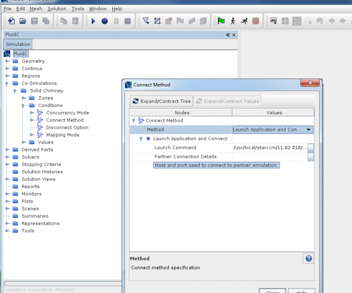
- Save the leading simulation and name it for example as lead.sim
Prepare Job Script
In the job script, use the following command to run the co-simulation:
starccm+ -np N,M -rsh /usr/local/bin/pbsrsh -batch -machinefile $PBS_NODEFILE lead.sim
where N is # of cores for the leading simulation and M is # of cores for the lagging simulation, and the summation of N and M should be the total number of cores you request in the job.
Once the job is completed, the output results of the leading simulation will be returned, while the lagging simulation runs on the background server and the final results won't be saved.
Supercomputer:
Service:
Fields of Science:
STAR-Fusion
STAR-Fusion is a component of the Trinity Cancer Transcriptome Analysis Toolkit (CTAT). STAR-Fusion uses the STAR aligner to identify candidate fusion transcripts supported by Illumina reads. STAR-Fusion further processes the output generated by the STAR aligner to map junction reads and spanning reads to a reference annotation set.
Availability and Restrictions
Versions
The following versions of STAR-Fusion are available on OSC clusters:
| Version | Owens |
|---|---|
| 0.7.0 | X* |
| 1.4.0 | X |
* Current default version
You can use module spider star-fusion to view available modules for a given machine. Feel free to contact OSC Help if you need other versions for your work.
Access
STAR-Fusion is available to all OSC users. If you have any questions, please contact OSC Help.
Publisher/Vendor/Repository and License Type
Broad Institute, Open source
Usage
Usage on Owens
Set-up
To configure your environment for use of STAR-Fusion, run the following command:
module load star-fusion. The default version will be loaded. To select a particular STAR-Fusion version, use module load star-fusion/version. For example, use module load star-fusion/0.7.0 to load STAR-Fusion 0.7.0.Further Reading
Supercomputer:
Service:
Fields of Science:
Salmon
Salmon is a tool for quantifying the expression of transcripts using RNA-seq data.
Availability and Restrictions
Versions
Salmon is available on the Owens Cluster. The versions currently available at OSC are:
| Version | Owens | Pitzer |
|---|---|---|
| 0.8.2 | X* | |
| 1.0.0 | X | |
| 1.2.1 | X | X* |
| 1.4.0 | X | |
| 1.10.0 | X |
* Current default version
You can use module spider salmonto view available modules for a given machine. Feel free to contact OSC Help if you need other versions for your work.
Access
Salmon is available to all OSC users. If you have any questions, please contact OSC Help.
Publisher/Vendor/Repository and License Type
Patro, R. et al., Freeware
Usage
Usage on Owens
Set-up
To configure your enviorment for use of Salmon, use command module load salmon. This will load the default version.
Further Reading
ScaLAPACK
ScaLAPACK is a library of high-performance linear algebra routines for clusters supporting MPI. It contains routines for solving systems of linear equations, least squares problems, and eigenvalue problems.
This page documents usage of the ScaLAPACK library installed by OSC from source. An optimized implementation of ScaLAPACK is included in MKL; see the software documentation page for Intel Math Kernel Library for usage information.
Availability and Restrictions
Versions
The versions currently available at OSC are:
| Version | Owens | Pitzer | Ascend |
|---|---|---|---|
| 2.0.2 | X | X | |
| 2.1.0 | X* | X* | |
| 2.2.0 | X* |
* Current default version
You can use module spider scalapack to view available modules for a given machine. Feel free to contact OSC Help if you need other versions for your work.
Access
ScaLAPACK is available to all OSC users. If you need high performance, we recommend using MKL instead of the standalone ScaLAPACK module. If you have any questions, please contact OSC Help.
Publisher/Vendor/Repository and License Type
Univ. of Tennessee; Univ. of California, Berkeley; Univ. of Colorado Denver; and NAG Ltd./ Open source
Usage
Usage on Owens
Set-up
Initalizing the system for use of the ScaLAPACK libraries is dependent on the system you are using and the compiler you are using. To use the ScaLAPACK libraries in your compilation, run the following command: module load scalapack. To load a particular version, use module load scalapack/version. For example, use module load scalapack/2.0.2 to load ScaLAPACK version 2.0.2. You can use module spider scalapack to view available modules.
Building with ScaLAPACK
Once loaded, the ScaLAPACK libraries can be linked in with your compilation. To do this, use the following environment variables. You must also link with MKL. With the Intel compiler, just add -mkl to the end of the link line. With other compilers, load the mkl module and add $MKL_LIBS to the end of the link line.
| Variable | Use |
|---|---|
$SCALAPACK_LIBS |
Used to link ScaLAPACK into either Fortran or C |
Usage on Pitzer
Set-up
Initalizing the system for use of the ScaLAPACK libraries is dependent on the system you are using and the compiler you are using. To use the ScaLAPACK libraries in your compilation, run the following command: module load scalapack. To load a particular version, use module load scalapack/version. For example, use module load scalapack/2.0.2 to load ScaLAPACK version 2.0.2. You can use module spider scalapack to view available modules.
Building with ScaLAPACK
Once loaded, the ScaLAPACK libraries can be linked in with your compilation. To do this, use the following environment variables. You must also link with MKL. With the Intel compiler, just add -mkl to the end of the link line. With other compilers, load the mkl module and add $MKL_LIBS to the end of the link line.
| VARIABLE | USE |
|---|---|
$SCALAPACK_LIBS |
Used to link ScaLAPACK into either Fortran or C |
Usage on Ascend
Set-up
Initalizing the system for use of the ScaLAPACK libraries is dependent on the system you are using and the compiler you are using. To use the ScaLAPACK libraries in your compilation, run the following command: module load scalapack. To load a particular version, use module load scalapack/version. For example, use module load scalapack/2.2.0 to load ScaLAPACK version 2.2.0. You can use module spider scalapack to view available modules.
Building with ScaLAPACK
Once loaded, the ScaLAPACK libraries can be linked in with your compilation. To do this, use the following environment variables. You must also link with MKL. With the Intel compiler, just add -mkl to the end of the link line. With other compilers, load the mkl module and add $MKL_LIBS to the end of the link line.
| VARIABLE | USE |
|---|---|
$SCALAPACK_LIBS |
Used to link ScaLAPACK into either Fortran or C |
Further Reading
Service:
Fields of Science:
Schrodinger
The Schrodinger molecular modeling software suite includes a number of popular programs focused on drug design and materials science but of general applicability, for example Glide, Jaguar, and MacroModel. Maestro is the graphical user interface for the suite. It allows the user to construct and graphically manipulate both simple and complex chemical structures, to apply molecular mechanics and dynamics techniques to evaluate the energies and geometries of molecules in vacuo or in solution, and to display and examine graphically the results of the modeling calculations.
Availability and Restrictions
Versions
The Schrodinger suite is available on Owens. The versions currently available at OSC are:
| Version | Owens |
|---|---|
| 15 | X |
| 16 | X |
| 2018.3 | X |
| 2019.3 | X |
| 2020.1 | X* |
* Current default version
You can use module spider schrodinger to view available modules for a given machine. Feel free to contact OSC Help if you need other versions for your work.
Access
Schrodinger is available to all academic users.
To use Schrodinger you will have to be added to the license server first. Please contact OSC Help to be added. Please note that if you are a non-OSU user, we need to send your name, contact email, and affiliation information to Schrodinger in order to grant access. Currently, we have license for following features:
CANVAS_ELEMENTS CANVAS_MAIN CANVAS_SHARED COMBIGLIDE_MAIN EPIK_MAIN FFLD_OPLS_MAIN GLIDE_MAIN GLIDE_XP_DESC IMPACT_MAIN KNIME_MAIN LIGPREP_MAIN MAESTRO_MAIN MMLIBS MMOD_CONFGEN MMOD_MACROMODEL MMOD_MBAE QIKPROP_MAIN
You need to use one of following software flags in order to use the particular feature of the software without license errors.
macromodel, glide, ligprep, qikprop, epik
You can add -L glide@osc:1 to your job script if you use GLIDE for example. When you use this software flag, then your job won't start until it secures available licenses. Please read the batch script examples below. You can check your license usage via the license usage checking tool.
Publisher/Vendor/Repository and License Type
Schrodinger, LLC/ Commercial
Usage
Usage on Owens
To set up your environment for schrodinger load one of its modulefiles:
module load schrodinger/2019.3
Using schrodinger interactively requires an X11 connection. Typically one will launch the graphical user interface maestro. This can be done with either software rendering:
maestro -SGL
or with hardware rendering:
module load vglrun
vglrun maestro
Note that hardware rendering requires a node with a GPU as well as the additional vglrun syntax above. In principle hardware rendering is superior; however, in practice it can be laggier, and thus software rendering can yield a better experience.
Here is an example batch script that uses schrodinger non-interactively via the batch system:
#!/bin/bash
# Example glide single node batch script.
#SBATCH --job-name=glidebatch
#SBATCH --time=1:00:00
#SBATCH --nodes=1 --ntasks-per-node=28
#SBATCH -L glide@osc:1
module load schrodinger
cp * $TMPDIR
cd $TMPDIR
host=`srun hostname|head -1`
nproc=`srun hostname|wc -l`
glide -WAIT -HOST ${host}:${nproc} -NJOBS 40 receptor_glide.in
ls -l
cp * $SLURM_SUBMIT_DIR
The glide command passes control to the Schrodinger Job Control utility which processes the two options: The WAIT option forces the glide command to wait until all tasks of the command are completed. This is necessary for the batch jobs to run effectively. The HOST option specifies how tasks are distributed over processors. In addition, the glide option NJOBS distributes the job into subjobs which can number more than the licenses or processors specified in the batch directives.
Further Reading
Supercomputer:
Service:
Fields of Science:
Scipion
SCIPION is an image processing framework fo robtaining 3D models of macromolecular complexes using Electron Microscopy (3DEM). It integrates several software packages and presents a unified interface for both biologists and developers. Scipion allows you to execute workflows combining different software tools, while taking care of formats and conversions. Additionally, all steps are tracked and can be reproduced later on.
Availability and Restrictions
Versions
The following versions are available on OSC clusters:
| Version | Pitzer |
|---|---|
| 3.0.8 | X* |
* Current default version
You can use module spider scipion to view available modules for a given machine. Feel free to contact OSC Help if you need other versions for your work.
Access
Scipion is available to all OSC users. If you have any questions, please contact OSC Help.
Publisher/Vendor/Repository and License Type
All scipion code and plugins, are licensed under the GPL3 (http://www.gnu.org/licenses/gpl-3.0.html)
Now, Scipion interacts, and in some cases installs 3rd party software with its own LICENCE that must be observed.
So, it is under the user responsibility to check the license of each of the software scipion is installing.
In most cases, if not all, software is free available for academic use and industry but there are few exceptions where industry users are not granted for a free usage. You must check each case.
Usage
Usage on Pitzer
Set-up
To configure your environment for use of scipion, run the following command: module load scipion. The default version will be loaded. To select a particular scipion version, use module load scipion/version. For example, use module load scipion/3.0.8 to load SCIPION 3.0.8
Scipion/3.0.8 was built with gnu/9.1.0, openmpi/4.0.3-hpcx, cuda/10.1.168, and hdf5/1.12.0.
Plugins
The following plugins are installed
scipion-em-xmipp scipion-em-resmap scipion-em-sphire scipion-em-localrec scipion-em-bsoft scipion-em-ccp4 scipion-em-cryoef scipion-em-spider scipion-em-imagic
Further Reading
Supercomputer:
Service:
Fields of Science:
SnpEff
SnpEff is a variant annotation and effect prediction tool. It annotates and predicts the effects of variants on genes (such as amino acid changes).
Availability and Restrictions
Versions
The following versions of SnpEff are available on OSC clusters:
| Version | Owens |
|---|---|
| 4.2 | X* |
* Current default version
You can use module spider snpeff to view available modules for a given machine. Feel free to contact OSC Help if you need other versions for your work.
Access
SnpEff is available to all OSC users. If you have any questions, please contact OSC Help.
Publisher/Vendor/Repository and License Type
http://snpeff.sourceforge.net, Open source
Usage
Usage on Owens
Set-up
To configure your environment for use of SnpEff, run the following command:
module load snpeff. The default version will be loaded. To select a particular SnpEff version, use module load snpeff/version. For example, use module load snpeff/4.2 to load SnpEff 4.2.Usage
This software consists of Java executable .jar files; thus, it is not possible to add to the PATH environment variable.
From module load snpeff, new environment variables, SNPEFF and SNPSIFT, will be set. Thus, users can use the software by running the following command: java -jar $SNPEFF {other options}, or java -jar $SNPSIFT {other options}.
Further Reading
Supercomputer:
Service:
Fields of Science:
Spark
Apache Spark is an open source cluster-computing framework originally developed in the AMPLab at University of California, Berkeley but was later donated to the Apache Software Foundation where it remains today. In contrast to Hadoop's disk-based analytics paradigm, Spark has multi-stage in-memory analytics. Spark can run programs up-to 100x faster than Hadoop’s MapReduce in memory or 10x faster on disk. Spark support applications written in python, java, scala and R
Availability and Restrictions
Versions
The following versions of Spark are available on OSC systems:
| Version | Owens | Pitzer | Note |
|---|---|---|---|
| 2.0.0 | X* | Only support Python 3.5 | |
| 2.1.0 | X | Only support Python 3.5 | |
| 2.3.0 | X | ||
| 2.4.0 | X | X* | |
| 2.4.5 | X | X |
* Current default version
You can use module spider spark to view available modules for a given machine. Feel free to contact OSC Help if you need other versions for your work.
Access
Spark is available to all OSC users. If you have any questions, please contact OSC Help.
Publisher/Vendor/Repository and License Type
The Apache Software Foundation, Open source
Usage
Set-up
In order to configure your environment for the usage of Spark, run the following command:
module load spark
A particular version of Spark can be loaded as follows
module load spark/2.3.0
Using Spark
In order to run Spark in batch, reference the example batch script below. This script requests 6 node on the Owens cluster for 1 hour of walltime. The script will submit the pyspark script called test.py using pbs-spark-submit command.
#!/bin/bash #SBATCH --job-name ExampleJob #SBATCH --nodes=2 --ntasks-per-node=48 #SBATCH --time=01:00:00 #SBTACH --account your_project_id module load spark cp test.py $TMPDIR cd $TMPDIR pbs-spark-submit test.py > test.log cp * $SLURM_SUBMIT_DIR
pbs-spark-submit script is used for submitting Spark jobs. For more options, please run,
pbs-spark-submit --help
Running Spark interactively in batch
To run Spark interactively, but in batch on Owens please run the following command,
sinteractive -N 2 -n 28 -t 01:00:00
When your interactive shell is ready, please launch spark cluster using the pbs-spark-submit script
pbs-spark-submit
You can then launch pyspark by connecting to Spark master node as follows.
pyspark --master spark://nodename.ten.osc.edu:7070
Launching Jupyter+Spark on OSC OnDemand
Instructions on how to launch Spark on OSC OnDemand web interface is here. https://www.osc.edu/content/launching_jupyter_spark_app
Custom Spark Property values
When launching a Spark application on Ondemand, users can provide a path to a custom property file that replaces Spark's default configuration settings. This allows for greater customization and optimization of Spark's behavior based on the specific needs of the application.
However, it's important to note that before setting the configuration using a custom property file, users should ensure that there are enough resources on the cluster to handle the requested configuration.
Example of custom property file:spark_custom.conf
spark.executor.instances 2 spark.executor.cores 2 spark.executor.memory 60g spark.driver.memory 2g
Users can check the default property values or the values after loading the custom property file as follows
spark.sparkContext.getConf().getAll()
Further Reading
See Also
Supercomputer:
Service:
Fields of Science:
Stata
Stata is a complete, integrated statistical package that provides everything needed for data analysis, data management, and graphics. 32-processor MP version is currently available at OSC.
Availability and Restrictions
Versions
The following versions of Stata are available on OSC systems:
| Version | Owens |
|---|---|
| 15 | X* |
| 17 | X |
* Current default version
You can use module spider stata to view available modules for a given machine. Feel free to contact OSC Help if you need other versions for your work.
Access
Only academic OSC users can use the software. OSC has the license for 5 seats concurrently. Each user can use up to 32 cores. In order to access the software, please contact OSC Help to get validated.
Publisher/Vendor/Repository and License Type
StataCorp, LLC, Commercial
Usage
Set-up
To configure your environment on Oakley for the usage of Stata, run the following command:
module load stata
Using Stata
Due to licensing restrictions, Stata may ONLY be used via the batch system on Owens. See below for information on how this is done.
Batch Usage
OSC has a 5-user license. However, there is no enforcement mechanism built into Stata. In order for us to stay within the 5-user limit, we require you to run in the context of Slurm and to include this option when starting your batch job (the Slurm system will enforce the 5 user limit):
#SBATCH -L stata@osc:1
Non-Interactive batch example
Use the script below as a template for your usage.
#!/bin/bash #SBATCH -t 1:00:00 #SBATCH --nodes=1 --ntask-per-node=28 #SBATCH -L stata@osc:1 #SBATCH --job-name=stata module load stata stata-mp -b do bigjob
Further Reading
See Also
Supercomputer:
Service:
Fields of Science:
StringTie
StringTie assembles aligned RNA-Seq reads into transcripts that represent splice variants in RNA-Seq samples.
Availability and Restrictions
Versions
StringTie is available on the Owens Cluster. The versions currently available at OSC are:
| Version | Owens |
|---|---|
| 1.3.3b | X* |
* Current Default Version
You can use module spider stringtieto view available modules for a given machine. Feel free to contact OSC Help if you need other versions for your work.
Access
StringTie is available to all OSC users. If you have any questions, please contact OSC Help.
Publisher/Vendor/Repository and License Type
https://ccb.jhu.edu/software/stringtie/, Open source
Usage
Usage on Owens
Set-up
To configure your enviorment for use of StringTie, use command module load stringtie. This will load the default version.
Further Reading
Supercomputer:
Fields of Science:
Subread
The Subread package comprises a suite of software programs for processing next-gen sequencing read data like Subread, Subjunc, featureCounts, and exactSNP.
Availability and Restrictions
Versions
The following versions of Subread are available on OSC clusters:
| Version | Owens |
|---|---|
| 1.5.0-p2 |
X* |
| 2.0.6 | X |
* Current default version
You can use module spider subread to view available modules for a given machine. Feel free to contact OSC Help if you need other versions for your work.
Access
Subread is available to all OSC users. If you have any questions, please contact OSC Help.
Publisher/Vendor/Repository and License Type
http://subread.sourceforge.net, Open source
Usage
Usage on Owens
Set-up
To configure your environment for use of Subread, run the following command:
module load subread. The default version will be loaded. To select a particular Subread version, use module load subread/version. For example, use module load subread/1.5.0-p2 to load Subread 1.5.0-p2.Further Reading
Supercomputer:
Service:
Fields of Science:
Subversion
Apache Subversion is a full-featured version control system.
Availability and Restrictions
Versions
The following versions of Subversion are available on OSC systems:
| Version | Owens |
|---|---|
| 1.8.19 | X* |
* Current default version
You can use module spider subversion to view available modules for a given machine. Feel free to contact OSC Help if you need other versions for your work.
Access
Subversion is available to all OSC users. If you have any questions, please contact OSC Help.
Publisher/Vendor/Repository and License Type
Apache Software Foundation, Open Source, Apache License
Usage
Set-up
The default version 1.7.14 is system-built. It is ready as you login. To use other versions, e.g 1.8.19 run the following command:
module load subversion/1.8.19
Further Reading
Tag:
Supercomputer:
Service:
Fields of Science:
SuiteSparse
SuiteSparse is a suite of sparse matrix algorithms, including: UMFPACK(multifrontal LU factorization), CHOLMOD(supernodal Cholesky, with CUDA acceleration), SPQR(multifrontal QR) and many other packages.
Availability and Restrictions
Versions
OSC supports most packages in SuiteSparse, including UMFPACK, CHOLMOD, SPQR, KLU and BTF, Ordering Methods (AMD, CAMD, COLAMD, and CCOLAMD) and CSparse. SuiteSparse modules are available for the Intel, GNU, and Portland Group compilers. The following versions of SuiteSparse are available at OSC.
| Version | Owens |
|---|---|
| 4.5.3 | X* |
* Current default version
You can use module spider suitesparse to view available modules for a given machine. Feel free to contact OSC Help if you need other versions for your work.
NOTE: SuiteSparse library on our clusters is built without METIS, which might matter if CHOLMOD package is included in your program.
Access
SuiteSparse is available to all OSC users. If you have any questions, please contact OSC Help.
Publisher/Vendor/Repository and License Type
Timothy A. Davis, Patrick R. Amestoy, and Iain S. Duff./ Open source
Usage
Usage on Owens
Set-up on Owens
To use SuitSparse, ensure the correct compiler is loaded. User module spider suitesparse/version to view compatible compilers. Before loading the SuiteSparse library, MKL is also required. Load the MKL library with module load mkl. Then with the following command, SuiteSparse library is ready to be used: module load suitesparse.
Building With SuiteSparse
With the SuiteSparse library loaded, the following environment variables will be available for use:
| Variable | Use |
|---|---|
| $SUITESPARSE_CFLAGS | Include flags for C or C++ programs. |
| $SUITESPARSE_LIBS | Use when linking your program to SuiteSparse library. |
For example, to build the code my_prog.c with the SuiteSparse library you would use:
icc -c my_prog.c icc -o my_prog my_prog.o $SUITESPARSE_LIBS
Batch Usage on Owens
When you log into oakley.osc.edu you are actually logged into a linux box referred to as the login node. To gain access to the mutiple processors in the computing environment, you must submit your job to the batch system for execution. Batch jobs can request mutiple nodes/cores and compute time up to the limits of the OSC systems. Refer to Queues and Reservations and Batch Limit Rules for more info. Batch jobs run on the compute nodes of the system and not on the login node. It is desirable for big problems since more resources can be used.
Non-interactive Batch Job (Serial Run)
A batch script can be created and submitted for a serial or parallel run. You can create the batch script using any text editor you like in a working directory on the system of your choice. You must load the SuiteSparse module in your batch script before executing a program which is built with the SuiteSparse library. Below is the example batch script that executes a program built with SuiteSparse:#!/bin/bash #SBATCH --job-name MyProgJob #SBATCH --nodes=1 --ntasks-per-node=28 #SBATCH --account <project-account> module load gnu/4.8.4 module load mkl module load suitesparse cp foo.dat $TMPDIR cd $TMPDIR my_prog < foo.dat > foo.out cp foo.out $SLURM_SUBMIT_DIR
Further Reading
See Also
Supercomputer:
Service:
Fields of Science:
TAU Commander
TAU Commander is a user interface for the TAU Performance System, a set of tools for analyizing the performance of parallel programs.
Availability and Restrictions
Versions
TAU Commander is available on the Owens Cluster. The versions currently available at OSC are:
| Version | Owens | Pitzer |
|---|---|---|
| 1.2.1 | X | |
| 1.3.0 | X* | X* |
* Current default version
You can use module spider taucmdr to view available modules for a given machine. Feel free to contact OSC Help if you need other versions for your work.
Access
TAU Commander is available to all OSC users. If you have any questions, please contact OSC Help.
Publisher/Vendor/Repository and License Type
ParaTools, Inc., Open source
Usage
Usage on Owens
Set-up
To configure your enviorment for use of TAU Commander, use command module load taucmdr. This will load the default version.
Creating a project
The first step to use TAU Commander on your code is to create and configure a project. To create a project, use the command tau initalize. Additional options for compilers, MPI libraries, measurements. etc. are available.
For instance, to configure for Intel compilers use the command tau initialize --compilers Intel and to configure for MPI use tau initialize --mpi.
For more details about how to initialize your project use the command tau help initialize.
After running creating the project you should see a dashboard for your project with a target, application, and 3 default measurements. You can now create additional measurements or modify the application and target. See the TAU Commander user guide for more information about how to configure your project.
Compiling and Running your Code
To compile your code to run with TAU Commander, just add tau before the compiler. For instance, if you are compiling with gcc now compile with tau gcc. Similarly, when you run your code add tau before the run command. So, if you usually run with srun -N 2 -n 4 ./my_prog now run with tau srun -N 2 -n 4 ./my_prog. Each time the program is run with tau prepended, a new trial is created in the project with performance data for that run.
Post-processing
Once you have generated performance data with TAU Commander you have 3 options to view the trial performance data:
- view the data in text format (not always available),
- view the data in a GUI using an OnDemand VDI (Virtual Desktop Interface) or X11 forwarding enabled,
- or export the data to your local machine (requires minimal installation of TAU commander on your local machine).
To view the data:
tau trial show trial_number
To export the data:
tau trial export trial_number
Usage on Pitzer
Set-up
To configure your enviorment for use of TAU Commander, use command module load taucmdr. This will load the default version.
Creating a project
The first step to use TAU Commander on your code is to create and configure a project. To create a project, use the command tau initalize. Additional options for compilers, MPI libraries, measurements. etc. are available.
For instance, to configure for Intel compilers use the command tau initialize --compilers Intel and to configure for MPI use tau initialize --mpi.
For more details about how to initialize your project use the command tau help initialize.
After running creating the project you should see a dashboard for your project with a target, application, and 3 default measurements. You can now create additional measurements or modify the application and target. See the TAU Commander user guide for more information about how to configure your project.
Compiling and Running your Code
To compile your code to run with TAU Commander, just add tau before the compiler. For instance, if you are compiling with gcc now compile with tau gcc. Similarly, when you run your code add tau before the run command. So, if you usually run with srun -N 2 -n 4 ./my_prog now run with tau srun -N 2 -n 4 -- ./my_prog. Each time the program is run with tau prepended, a new trial is created in the project with performance data for that run. See man srun or the srun documenation for information on arguements used above.
Post-processing
Once you have generated performance data with TAU Commander you have 3 options to view the trial performance data:
- view the data in text format (not always available),
- view the data in a GUI using an OnDemand VDI (Virtual Desktop Interface) or X11 forwarding enabled,
- or export the data to your local machine (requires minimal installation of TAU commander on your local machine).
To view the data:
tau trial show trial_number
To export the data:
tau trial export trial_number
Further Reading
TensorFlow
"TensorFlow is an open source software library for numerical computation using data flow graphs. Nodes in the graph represent mathematical operations, while the graph edges represent the multidimensional data arrays (tensors) that flow between them. This flexible architecture lets you deploy computation to one or more CPUs or GPUs in a desktop, server, or mobile device without rewriting code."
Quote from TensorFlow Github documentation.
Availability and Restrictions
Versions
The following version of TensorFlow is available on OSC clusters:
| Version | Owens | Pitzer | Note | CUDA version compatibility |
|---|---|---|---|---|
| 1.3.0 | X | python/3.6 | 8 or later | |
| 1.9.0 | X* | X* | python/3.6-conda5.2 | 9 or later |
| 2.0.0 | X | X | python/3.7-2019.10 | 10.0 or later |
TensorFlow is a Python package and therefore requires loading corresonding python modules (see Note). The version of TensorFlow may actively change with updates to Anaconda Python on Owens so that you can check the latest version with conda list tensorflow. The available versions of TensorFlow on Owens and Pitzer require CUDA for GPU calculations. You can find and load compatible cuda module via
module load python/3.6-conda5.2 module spider cuda module load cuda/9.2.88
If you would like to use a different version of TensorFlow, please follow this installation guide which describes how to install python packages locally.
https://www.osc.edu/resources/getting_started/howto/howto_install_tensorflow_locally
Newer version of TensorFlow might require newer version of CUDA. Please refer to https://www.tensorflow.org/install/source#gpu for a up-to-date compatibility chart.
Feel free to contact OSC Help if you have any issues with installation.
Access
TensorFlow is available to all OSC users. If you have any questions, please contact OSC Help.
Publisher/Vendor/Repository and License Type
https://www.tensorflow.org, Open source
Usage on Owens
Usage on Owens
Setup on Owens
TensorFlow package is installed using Anaconda Python 2. To configure the Owens cluster for the use of TensorFlow, use the following commands:
module load python/3.6 cuda/8.0.44
Batch Usage on Ruby or Owens
Batch jobs can request multiple nodes/cores and compute time up to the limits of the OSC systems. Refer to Queues and Reservations for Owens, and Scheduling Policies and Limits for more info. In particular, TensorFlow should be run on a GPU-enabled compute node.
An Example of Using TensorFlow with MNIST model and Logistic Regression
Below is an example batch script (job.txt and logistic_regression_on_mnist.py) for using TensorFlow.
Contents of job.txt
#!/bin/bash #SBATCH --job-name ExampleJob #SBATCH --nodes=2 --ntasks-per-node=28 --gpus-per-node=1 #SBATCH --time=01:00:00 cd $PBS_O_WORKDIR module load python/3.6 cuda/8.0.44 python logistic_regression_on_mnist.py
Contents of logistic_regression_on_mnist.py
# logistic_regression_on_mnist.py Python script based on:
# https://github.com/aymericdamien/TensorFlow-Examples/blob/master/notebooks/0_Prerequisite/mnist_dataset_intro.ipynb
# https://github.com/aymericdamien/TensorFlow-Examples/blob/master/notebooks/2_BasicModels/logistic_regression.ipynb
import tensorflow as tf
# Import MNIST
from tensorflow.examples.tutorials.mnist import input_data
mnist = input_data.read_data_sets("data/", one_hot=True)
# Parameters
learning_rate = 0.01
training_epochs = 25
batch_size = 100
display_step = 1
# tf Graph Input
x = tf.placeholder(tf.float32, [None, 784]) # mnist data image of shape 28*28=784
y = tf.placeholder(tf.float32, [None, 10]) # 0-9 digits recognition => 10 classes
# Set model weights
W = tf.Variable(tf.zeros([784, 10]))
b = tf.Variable(tf.zeros([10]))
# Construct model
pred = tf.nn.softmax(tf.matmul(x, W) + b) # Softmax
# Minimize error using cross entropy
cost = tf.reduce_mean(-tf.reduce_sum(y*tf.log(pred), reduction_indices=1))
# Gradient Descent
optimizer = tf.train.GradientDescentOptimizer(learning_rate).minimize(cost)
# Initializing the variables
init = tf.global_variables_initializer()
# Launch the graph
with tf.Session() as sess:
sess.run(init)
# Training cycle
for epoch in range(training_epochs):
avg_cost = 0.
total_batch = int(mnist.train.num_examples/batch_size)
# Loop over all batches
for i in range(total_batch):
batch_xs, batch_ys = mnist.train.next_batch(batch_size)
# Fit training using batch data
_, c = sess.run([optimizer, cost], feed_dict={x: batch_xs,
y: batch_ys})
# Compute average loss
avg_cost += c / total_batch
# Display logs per epoch step
if (epoch+1) % display_step == 0:
print ("Epoch:", '%04d' % (epoch+1), "cost=", "{:.9f}".format(avg_cost))
print ("Optimization Finished!")
# Test model
correct_prediction = tf.equal(tf.argmax(pred, 1), tf.argmax(y, 1))
# Calculate accuracy for 3000 examples
accuracy = tf.reduce_mean(tf.cast(correct_prediction, tf.float32))
print ("Accuracy:", accuracy.eval({x: mnist.test.images[:3000], y: mnist.test.labels[:3000]}))
In order to run it via the batch system, submit the job.txt file with the following command:
sbatch job.txt
Distributed Tensorflow
Tensorflow can be configured to run parallel using Horovod package from uber.
Further Reading
Tag:
Supercomputer:
Service:
Technologies:
Fields of Science:
Texlive
TeX Live is a straightforward way to get up and running with the TeX document production system. It provides a comprehensive TeX system with binaries for most flavors of Unix, including GNU/Linux, macOS, and also Windows. It includes all the major TeX-related programs, macro pacakges, and fonts that are free software, including support for many languages around the world.
Availability and Restrictions
Versions
The following versions are available on OSC clusters:
| Version | Owens | Pitzer |
|---|---|---|
| 2018 | X* | X* |
| 2021 | X | X |
* Current default version
You can use module spider texlive to view available modules for a given machine. Feel free to contact OSC Help if you need other versions for your work.
Access
Texlive is available to all OSC users. If you have any questions, please contact OSC Help.
Publisher/Vendor/Repository and License Type
Per the TeX Live licensing, copying, and redistribution webpage, all the material in TeX Live may be freely used, copied, modified, and/or redistributed, subject to (in many cases) the sources remaining freely available.
Please visit this link for full licensing/copyright information.
Usage
Usage on Owens
Set-up
To configure your environment for use of mriqc, run the following command: module load texlive. The default version will be loaded. To select a particular Texlive version, use module load texlive/version. For example, use module load texlive/2021 to load Texlive 2021.
Usage on Pitzer
Set-up
To configure your environment for use of mriqc, run the following command:module load texlive. The default version will be loaded. To select a particular Texlive version, use module load texlive/version. For example, use module load texlive/2021 to load Texlive 2021.Further Reading
Tag:
Service:
Technologies:
Fields of Science:
Tinker
Tinker is a molecular modeling package. Tinker provides a general set of tools for molecular mechanics and molecular dynamics.
Availability and Restrictions
Versions
Tinker is currently available on Owens and Pitzer. The versions currently available at OSC are:
| Version | Owens | Pitzer |
|---|---|---|
| 8.10.5 | X* | X* |
* Current default version
You can use module spider tinker to view available modules for a given machine. Feel free to contact OSC Help if you need other versions for your work.
Access
Tinker is available to all OSC users. If you have any questions, please contact OSC Help.
Publisher/Vendor/Repository and License Type
Tinker Core Development Consortium
Usage
Usage on Owens
Set-up
To configure your environment for use of Tinker, you first need to load the correct compiler. Use module spider tinker to see the compatable compilers. Then load a compatable compiler by runningmodule load compiler/version.
Then use the command module load tinker. This will load the default version of Tinker. To select a particular version, use module load tinker/version .
For example, execute module load intel/2021.3.0 then module load tinker/8.10.5 to load Tinker version 8.10.5 on Owens.
Usage on Pitzer
Set-up
To configure your environment for use of Tinker, you first need to load the correct compiler. Use module spider tinker to see the compatable compilers. Then load a compatable compiler by runningmodule load compiler/version.
Then use the command module load tinker. This will load the default version of Tinker. To select a particular version, use module load tinker/version .
For example, execute module load intel/2021.3.0 then module load tinker/8.10.5 to load Tinker version 8.10.5 on Pitzer.
Further Reading
Fields of Science:
TopHat
TopHat uses Bowtie, a high-throughput short read aligner, to analyze the mapping results for RNA-Seq reads and identify splice junctions.
Please note that tophat (and bowtie) cannot run in parallel, that is, on multiple nodes. Submitting multi-node jobs will only waste resources. In addition you must explicitly include the '-p' option to use multiple threads on a single node.
Availability and Restrictions
Versions
TopHat is available on the Owens Cluster. The versions currently available at OSC are:
| Version | Owens |
|---|---|
| 2.1.1 | X* |
* Current default version
You can use module spider tophat to view available modules for a given machine. Feel free to contact OSC Help if you need other versions for your work.
Access
TopHat is available to all OSC users. If you have any questions, please contact OSC Help.
Publisher/Vendor/Repository and License Type
http://ccb.jhu.edu/software/tophat, Open source
Usage
Usage on Owens
Set-up
To configure your enviorment for use of TopHat, use command module load tophat. This will load the default version.
Further Reading
Supercomputer:
Fields of Science:
Torch
"Torch is a deep learning framework with wide support for machine learning algorithms. It's open-source, simple to use, and efficient, thanks to an easy and fast scripting language, LuaJIT, and an underlying C / CUDA implementation. Torch offers popular neural network and optimization libraries that are easy to use, yet provide maximum flexibility to build complex neural network topologies. It also runs up to 70% faster on the latest NVIDIA Pascal™ GPUs, so you can now train networks in hours, instead of days."
Quote from Torch documentation.
Availability and Restrictions
Versions
The following version of Torch is available on OSC cluster:
| Version | Owens |
|---|---|
| 7 | X* |
* Current default version
You can use module spider torch to view available modules for a given machine. Feel free to contact OSC Help if you need other versions for your work.
The current version of Torch on Owens requires cuda/8.0.44 and CUDNN v5 for GPU calculations.
Access
Torch is available to all OSC users. If you have any questions, please contact OSC Help.
Publisher/Vendor/Repository and License Type
Soumith Chintala, Ronan Collobert, Koray Kavukcuoglu, Clement Farabet/ Open source
Usage
Usage on Owens
Setup on Owens
To configure the Owens cluster for the use of Torch, use the following commands:
module load torch
Batch Usage on Ruby or Owens
Batch jobs can request multiple nodes/cores and compute time up to the limits of the OSC systems. Refer to Queues and Reservations for Owens, and Scheduling Policies and Limits for more info. In particular, Torch should be run on a GPU-enabled compute node.
An Example of Using Torch with CIFAR10 Training Data on Owens
Below is an example batch script (job.txt) for using Torch. Please see the reference https://github.com/szagoruyko/cifar.torch for more details.
#!/bin/bash
#SBATCH --job-name=Torch
#SBATCH --nodes=1 --ntasks-per-node=28 --gpus=1
#SBATCH --time=00:30:00
#SBATCH --account <project-account>
# Load module load for torch
module load torch
# Migrate to job temp directory
cd $TMPDIR
# Clone sample data and scripts
git clone https://github.com/szagoruyko/cifar.torch.git .
# Run the image preprocessing (not necessary for subsequent runs, just re-use provider.t7)
OMP_NUM_THREADS=28 th -i provider.lua <<Input
provider = Provider()
provider:normalize()
torch.save('provider.t7',provider)
exit
y
Input
# Run the torch training
th train.lua --backend cudnn
# Copy results from job temp directory
cp -a * $SLURM_SUBMIT_DIR
In order to run it via the batch system, submit the job.txt file with the following command:
sbatch job.txt
Further Reading
Tag:
Supercomputer:
Service:
Technologies:
Fields of Science:
Transmission3d
Transmission3d is a 3-dimensional, multi-body gear contact analysis software capable of modeling complex gear systems developed by Ansol (Advanced Numeric Solutions). Multiple gear types, including: Helical, Straight Bevel, Spiral Bevel, Hypoids, Beveloids and Worms can be modeled. Multiple bearing types, as well as complex shafts, carriers and housings can also be modeled with the software. A variety of output data options including tooth bending stress, contact patterns, and displacement are also available.
Availability and Restrictions
Versions
The following versions of Blender are available on OSC systems:
|
VERSION |
OWENS |
|---|---|
|
6724 |
X* |
* Current default version
Access
Contact OSC Help and Ansol sales to get access to Transmission3D.
Publisher/Vendor/Repository and License Type
Ansol, Commercial
Further Reading
Tag:
Supercomputer:
Service:
Fields of Science:
TrimGalore
TrimGalore is a wrapper tool that automates quality and adapter trimming to FastQ files. It also provides functionality to RRBS sequence files.
Availability and Restrictions
Versions
TrimGalore is available on the Owens cluster. The versions currently available at OSC are:
| Version | Owens |
|---|---|
| 0.4.5 | X* |
* Current default version
You can use module spider trimgalore to view available modules for a given machine. Feel free to contact OSC Help if you need other versions for your work.
Access
TrimGalore is available to all OSC users. If you have any questions, please contact OSC Help.
Publisher/Vendor/Repository and License Type
The Babraham Institute, Open source
Usage
Usage on Owens
Set-up
To configure your enviorment for use of TrimGalore, use command module load trimgalore. This will load the default version.
Further Reading
Supercomputer:
Fields of Science:
Trimmomatic
Trimmomatic performs a variety of useful trimming tasks for illumina paired-end and single ended data.The selection of trimming steps and their associated parameters are supplied on the command line.
Availability and Restrictions
Versions
The following versions of Trimmomatic are available on OSC clusters:
| Version | Owens | Pitzer |
|---|---|---|
| 0.36 | X* | |
| 0.38 | X* |
* Current default version
You can use module spider trimmomatic to view available modules for a given machine. Feel free to contact OSC Help if you need other versions for your work.
Access
Trimmomatic is available to all OSC users. If you have any questions, please contact OSC Help.
Publisher/Vendor/Repository and License Type
http://www.usadellab.org/cms/?page=trimmomatic, Open source
Usage
Usage on Owens
Set-up
To configure your environment for use of Trimmomatic, run the following command:
module load trimmomatic. The default version will be loaded. To select a particular Trimmomatic version, use module load trimmomatic/version. For example, use module load trimmomatic/0.36 to load Trimmomatic 0.36.Usage
This software is a Java executable .jar file; thus, it is not possible to add to the PATH environment variable.
From module load trimmomatic, a new environment variable, TRIMMOMATIC, will be set.
Thus, users can use the software by running the following command: java -jar $TRIMMOMATIC {other options}.
Usage on Pitzer
Set-up
To configure your environment for use of Trimmomatic, run the following command:
module load trimmomatic. The default version will be loaded. To select a particular Trimmomatic version, use module load trimmomatic/version. For example, use module load trimmomatic/0.38 to load Trimmomatic 0.38.Usage
This software is a Java executable .jar file; thus, it is not possible to add to the PATH environment variable.
From module load trimmomatic, a new environment variable, TRIMMOMATIC, will be set.
Thus, users can use the software by running the following command: java -jar $TRIMMOMATIC {other options}.
Further Reading
Service:
Fields of Science:
Trinity
Trinity represents a novel method for the efficient and robust de novo reconstruction of transcriptomes from RNA-seq data.
Availability and Restrictions
The following versions of Trinity are available on OSC clusters:
| Version | Owens | Pitzer |
|---|---|---|
| 2.11.0 | X | X |
| 2.15.1 | X |
* Current default version
You can use module spider trinityrnaseq to view available modules for a given machine. Feel free to contact OSC Help if you need other versions for your work.
Access
Trinity is available to all OSC users. If you have any questions, please contact OSC Help.
Publisher/Vendor/Repository and License Type
Broad Institute and the Hebrew University of Jerusalem, Open source
Usage
Usage on Pitzer and Owens
Set-up
To configure your environment for use of Trinity, run the following command:
module load trinityrnaseq. The default version will be loaded. To select a particular Trinity version, use module load trinityrnaseq/version. For example, use module load trinityrnaseq/2.11.0 to load Trinity 2.11.0.Further Reading
Service:
Fields of Science:
TurboVNC
TurboVNC is an implementation of VNC optimized for 3D graphics rendering. Like other VNC software, TurboVNC can be used to create a virtual desktop on a remote machine, which can be useful for visualizing CPU-intensive graphics produced remotely.
Availability and Restrictions
Versions
The versions currently available at OSC are:
| Version | Owens | Pitzer | Notes |
|---|---|---|---|
| 2.0.91 | X | ||
| 2.1.1 | X | Must load intel compiler, version 16.0.3 for Owens | |
| 2.1.90 | X* | X* |
* Current default version
NOTE:
- [1] -- TurboVNC 1.1's version of vncviewer does not work on Oakley. Use the 1.2 module's version.
- [2] -- TurboVNC 1.2's version of vncserver does not work on Oakley. Use the 1.1 module's version.
- To simplify vncviewer and vncserver incompatibility with prior 1.X versions, a new version of TurboVNC 2.0 is available as of 10/30/2015 on Oakley and Ruby clusters.
- A version of TurboVNC 2.0.91 was installed in September 2016 to be uniformly available on all OSC clusters.
You can use module spider turbovnc to view available modules for a given cluster. Feel free to contact OSC Help if you need other versions for your work.
Access
TurboVNC is available for use by all OSC users.
Publisher/Vendor/Repository and License Type
https://www.turbovnc.org, Open source
Usage
Usage on Owens
Setup on Owens
To load the default version of TurboVNC module, use module load turbovnc. To select a particular software version, use module load turbovnc/version. For example, use module load turbovnc/2.0 to load TurboVNC version 2.0 on Oakley.
Please do not SSH directly to compute nodes and start VNC sessions! This will negatively impact other users (even if you have been assigned a node via the batch scheduler), and we will consider repeated occurances an abuse of the resources. If you need to use VNC on a compute node, please see our HOWTO for instructions.
Using TurboVNC
To start a VNC server on your current host, use the following command:
vncserver
After starting the VNC server you should see output similar to the following:
New 'X' desktop is hostname:display Starting applications specified in /nfs/nn/yourusername/.vnc/xstartup.turbovnc Log file is /nfs/nn/yourusername/.vnc/hotsname:display.log
Make a note of the hostname and display number ("hostname:display"), because you will need this information later in order to connect to the running VNC server.
To establish a standard unencrypted connection to an already running VNC server, X11 forwarding must first be enabled in your SSH connection. This can usually either be done by changing the preferences or settings in your SSH client software application, or by using the -X or -Y option on your ssh command.
Once you are certain that X11 forwarding is enabled, create your VNC desktop using the vncviewer command in a new shell.
vncviewer
You will be prompted by a dialogue box asking for the VNC server you wish to connect to. Enter "hostname:display".
You may then be prompted for your HPC password. Once the password has been entered your VNC desktop should appear, where you should see all of your home directory contents.
When you are finished with your work on the VNC desktop, you should make sure to close the desktop and kill the VNC server that was originally started. The VNC server can be killed using the following command in the shell where the VNC server was originally started:
vncserver -kill :[display]
For a full explanation of each of the previous commands, type man vncserver or man vncviewer at the command line to view the online manual.
Usage on Pitzer
Setup on Pitzer
To load the default version of TurboVNC module, use module load turbovnc.
Please do not SSH directly to compute nodes and start VNC sessions! This will negatively impact other users (even if you have been assigned a node via the batch scheduler), and we will consider repeated occurances an abuse of the resources. If you need to use VNC on a compute node, please see our HOWTO for instructions.
Using TurboVNC
To start a VNC server on your current host, use the following command:
vncserver
After starting the VNC server you should see output similar to the following:
New 'X' desktop is hostname:display Starting applications specified in /nfs/nn/yourusername/.vnc/xstartup.turbovnc Log file is /nfs/nn/yourusername/.vnc/hotsname:display.log
Make a note of the hostname and display number ("hostname:display"), because you will need this information later in order to connect to the running VNC server.
To establish a standard unencrypted connection to an already running VNC server, X11 forwarding must first be enabled in your SSH connection. This can usually either be done by changing the preferences or settings in your SSH client software application, or by using the -X or -Y option on your ssh command.
Once you are certain that X11 forwarding is enabled, create your VNC desktop using the vncviewer command in a new shell.
vncviewer
You will be prompted by a dialogue box asking for the VNC server you wish to connect to. Enter "hostname:display".
You may then be prompted for your HPC password. Once the password has been entered your VNC desktop should appear, where you should see all of your home directory contents.
When you are finished with your work on the VNC desktop, you should make sure to close the desktop and kill the VNC server that was originally started. The VNC server can be killed using the following command in the shell where the VNC server was originally started:
vncserver -kill :[display]
For a full explanation of each of the previous commands, type man vncserver or man vncviewer at the command line to view the online manual.
Further Reading
Additional information about TurboVNC can be found at the VirtualGL Project's documentation page.
See Also
Service:
Fields of Science:
Turbomole
TURBOMOLE is an ab initio computational chemistry program that implements various quantum chemistry algorithms. It is focused on efficiency, notably using the resolution of the identity (RI) approximation.
Availability and Restrictions
Versions
These versions are currently available (S means serial executables, O means OpenMP executables, and P means parallel MPI executables):
| Version | Owens | Pitzer |
|---|---|---|
| 7.1 | SOP | |
| 7.2.1 | SOP* | |
| 7.3 | SOP* |
* Current default version
You can use module spider turbomole to view available modules for a given machine. Feel free to contact OSC Help if you need other versions for your work.
Access for Academic Users
Use of Turbomole for academic purposes requires validation. In order to obtain validation, please contact OSC Help for further instruction.
Publisher/Vendor/Repository and License Type
COSMOlogic, Commercial
Usage
Usage on Owens and Pitzer
Set-up on Owens
To load the default version of Turbomole module on Owens, usemodule load turbomole for both serial and parallel programs. To select a particular software version, use module load turbomole/version. For example, use module load turbomole/7.1 to load Turbomole version 7.1 for both serial and parallel programs on Owens.
Using Turbomole on Owens
To execute a turbomole program:
module load turbomole <turbomole command>
Batch Usage on Owens
When you log into owens.osc.edu you are actually logged into a linux box referred to as the login node. To gain access to the mutiple processors in the computing environment, you must submit your job to the batch system for execution. Batch jobs can request mutiple nodes/cores and compute time up to the limits of the OSC systems. Refer to Queues and Reservations and Batch Limit Rules for more info. Batch jobs run on the compute nodes of the system and not on the login node. It is desirable for big problems since more resources can be used.
Interactive Batch Session
For an interactive batch session one can run the following command:
qsub -I -l nodes=1:ppn=28 -l walltime=00:20:00
which requests 28 cores (-l nodes=1:ppn=28), for a walltime of 20 minutes (-l walltime=00:20:00). You may adjust the numbers per your need.
Sample batch scripts and input files are available here:
~srb/workshops/compchem/turbomole/
Note for Slurm job script
Upon Slurm migration, the presets for parallel jobs are not compatiable with Slurm environment of Pitzer. Users must set up parallel environment explicitly to get correct TURBOMOLE binaries.
To set up a MPI case, add the following to a job script:
export PARA_ARCH=MPI export PATH=$TURBODIR/bin/`sysname`:$PATH
An example script:
#!/bin/bash #SBATCH --job-name="turbomole_mpi_job" #SBATCH --nodes=2 #SBATCH --time=0:10:0 module load intel module load turbomole/7.3 export PARA_ARCH=MPI export PATH=$TURBODIR/bin/`sysname`:$PATH export PARNODES=$SLURM_NTASKS dscf
To set up a SMP (OpenMP) case, add the following to a job script:
export PARA_ARCH=SMP export PATH=$TURBODIR/bin/`sysname`:$PATH
An example script to run a SMP job on an exclusive node:
#!/bin/bash #SBATCH --job-name="turbomole_smp_job" #SBATCH --nodes=1 #SBATCH --exclusive #SBATCH --time=0:10:0 module load intel module load turbomole/7.3 export PARA_ARCH=SMP export PATH=$TURBODIR/bin/`sysname`:$PATH export OMP_NUM_THREADS=$SLURM_CPUS_ON_NODE dscf
Further Reading
Service:
Fields of Science:
USEARCH
USEARCH is a sequence analysis tool that offers high-throughput search and clustering algorithms to analyze data.
Availability and Restrictions
Versions
USEARCH is available on the Owens cluster. The versions currently available at OSC are:
| Version | Owens |
|---|---|
| 10.0.240 | X* |
* Current Default Version
You can use module spider usearch to view available modules for a given machine. Feel free to contact OSC Help if you need other versions for your work.
Access
USEARCH is available to all academic OSC users.
Publisher/Vendor/Repository and License Type
drive5, Commercial
Usage
Usage on Owens
Further Reading
Supercomputer:
Unblur
Unblur is used to align the frames of movies recorded on an electron microscope to reduce image blurrig due to beam-induced motion. It reads stacks of movies that are stored in MRC/CCP4 format. Unblur generates frame sums that can be used in subsequent image processing steps and optionally applies an exposure-dependent filter to maximize the signal at all resolutions in the frame averages. Movie frame sums can also be calculated using Summovie, which uses the alignment resuls from a prior run of Unblur.
Availability & Restrictions
Versions
The following version of Boost are available on OSC systems:
| Version | Pitzer |
|---|---|
| 1.0.2 |
You can use module spider unblur to view available modules for a given machine. Feel free to contact OSC Help if you need other versions for your work.
Access
Unblur is available to all OSC users. If you have any questions, please contact OSC Help.
Publisher/Vendor/Repository and License Type
This software is subject to Janelia Farm Research Campus Software Copyright 1.1. Full details of this license can be found using this link.
Usage
Usage on Pitzer
Set-up
To configure your environment for use of Unblur, run the following command: module load unblur. The default version will be loaded.
To select a particular Unblur version, use module load unblur/version. For example, use module load unblur/1.0.2 to load Unblur 1.0.2.
Further Reading
Supercomputer:
Service:
Fields of Science:
VASP
The Vienna Ab initio Simulation Package, VASP, is a suite for quantum-mechanical molecular dynamics (MD) simulations and electronic structure calculations.
Availability and Restrictions
Access
Due to licensing considerations, OSC does not provide general access to this software.
However, we are available to assist with the configuration of individual research-group installations on all our clusters. See the VASP FAQ page for information regarding licensing.
Usage
Using VASP
See the VASP documentation page for tutorial and workshop materials.
Building and Running VASP
If you have a VASP license you may build and run VASP on any OSC cluster. The instructions given here are for VASP 5.4.1; newer 5 versions should be similar; and we have several reports that these worked for VASP 6.3.2.
Most VASP users at OSC run VASP with MPI and without multithreading. If you need assistance with a different configuration, please contact oschelp@osc.edu. Note that we recommend submitting a batch job for testing because running parallel applications from a login node is problematic.
You can build and run VASP using either IntelMPI or MVAPICH2. Performance is similar for the two MPI families. Instructions are given for both. The IntelMPI build is simpler and more standard. MVAPICH2 is the default MPI installation at OSC; however, VASP had failures with some prior versions, so building with the newest MVAPICH2, in particular 2.3.2 or newer, is recommended.
Build instructions assume that you have already unpacked the VASP distribution and patched it if necessary and are working in the vasp directory. It also assumes that you have the default module environment loaded at the start.
Building with IntelMPI
1. Copy arch/makefile.include.linux_intel and rename it makefile.include.
2. Edit makefile.include to replace the two lines
OBJECTS = fftmpiw.o fftmpi_map.o fftw3d.o fft3dlib.o \ $(MKLROOT)/interfaces/fftw3xf/libfftw3xf_intel.a
with one line
OBJECTS = fftmpiw.o fftmpi_map.o fftw3d.o fft3dlib.o
3. Make sure the FCL line is
FCL = mpiifort -mkl=sequential
4. Load modules and build the code (using the latest IntelMPI may yield the best performance; for VASP 5.4.1 the modules were intel/19.0.5 and intelmpi/2019.3 as of October 2019)
module load intelmpi make
5. Add the modules used for the build, e.g., module load intelmpi, to your job script.
Building with MVAPICH2
1. Copy arch/makefile.include.linux_intel and rename it makefile.include.
2. Edit makefile.include to replace mpiifort with mpif90
FC = mpif90 FCL = mpif90 -mkl=sequential
3. Replace the BLACS, SCALAPACK, OBJECTS, INCS and LLIBS lines with
BLACS = SCALAPACK = $(SCALAPACK_LIBS) OBJECTS = fftmpiw.o fftmpi_map.o fftw3d.o fft3dlib.o INCS = $(FFTW3_FFLAGS) LLIBS = $(SCALAPACK) $(FFTW3_LIBS_MPI) $(LAPACK) $(BLAS)
4. Load modules and build the code (using the latest MVAPICH2 is recommended; for VASP 5.4.1 the modules were intel/19.0.5 and mvapich2/2.3.2 as of October 2019)
module load scalapack module load fftw3 make
5. Add the modules used for the build, e.g., module load scalapack fftw3, to your job script.
Building for GPUs
The "GPU Stuff" section in arch/makefile.include.linux_intel_cuda is generic. It can be updated for OSC clusters using the environment variables defined by a cuda module. The OSC_CUDA_ARCH environment variables defined by cuda modules on all clusters show the specific CUDA compute capabilities. Below we have combined them as of February 2023 so that the resulting executable will run on any OSC cluster. In addition to the instructions above, here are the specific CUDA changes and the commands for building a gpu executable.
Edits:
CUDA_ROOT = $(CUDA_HOME)
GENCODE_ARCH = -gencode=arch=compute_35,code=\"sm_35,compute_35\" \
-gencode=arch=compute_60,code=\"sm_60,compute_60\" \
-gencode=arch=compute_70,code=\"sm_70,compute_70\" \
-gencode=arch=compute_80,code=\"sm_80,compute_80\"
Commands:
module load cuda make gpu
See this VASP Manual page and this NVIDIA page for reference.
Running VASP generally
Be sure to load the appropriate modules in your job script based on your build configuration, as indicated above. If you have built with -mkl=sequential you should be able to run VASP as follows:
mpiexec path_to_vasp/vasp_std
If you have a problem with too many threads you may need to add this line (or equivalent) near the top of your script:
export OMP_NUM_THREADS=1
Running VASP with GPUs
See this VASP Manual page and this NVIDIA page for feature restrictions, input requirements, and performance tuning examples. To acheive maximum performance, benchmarking of your particular calculation is essential. As a point of reference, although GPUs are the scarce resource, some user reports are that optimal performance is with 3 or 4 MPI ranks per GPU. This is expected to depend on method and simulation size.
If you encounter a CUDA error running a GPU enabled executable, such as:
CUDA Error in cuda_mem.cu, line 44: all CUDA-capable devices are busy or unavailable
then you may need to use the default compute mode which can be done by adding this line (or equivalent) near the top of your script, e.g., for Owens:
#SBATCH --nodes=1 --ntasks-per-node=28 --gpus-per-node=1 --gpu_cmode=shared
Known Issues
VASP job with Out-of-Memory crashes Owens Compute nodes
There is a bug with VASP 5.4.1 built with mvapich2/2.2 on Owens such that the VASP job with out-of-memory issue crashes the Owens compute node(s). We suggest to use a newer version of VASP.
Further Reading
See Also
Service:
Fields of Science:
VCFtools
VCFtools is a program package designed for working with VCF files, such as those generated by the 1000 Genomes Project. The aim of VCFtools is to provide easily accessible methods for working with complex genetic variation data in the form of VCF files.
Availability and Restrictions
The following versions of VCFtools are available on OSC clusters:
| Version | Owens | Pitzer |
|---|---|---|
| 0.1.14 | X | X |
| 0.1.16 | X* | X* |
* Current default version
You can use module spider vcftools to view available modules for a given machine. Feel free to contact OSC Help if you need other versions for your work.
Access
VCFtools is available to all OSC users. If you have any questions, please contact OSC Help.
Publisher/Vendor/Repository and License Type
Adam Auton, Petr Danecek, Anthony Marcketta/ Open source
Usage
Usage on Owens
Set-up
To configure your environment for use of VCFtools, run the following command:
module load vcftools. The default version will be loaded. To select a particular VCFtools version, use module load vcftools/version . For example, use module load vcftools/0.1.14 to load VCFtools 0.1.14.Usage on Pitzer
Set-up
To configure your environment for use of VCFtools, run the following command:
module load vcftools. The default version will be loaded.Further Reading
Service:
Fields of Science:
VMD
VMD is a visulaization program for the display and analysis of molecular systems.
Availability and Restrictions
Versions
The following versions of VMD are available on OSC clusters:
| Version | Owens | Pitzer |
|---|---|---|
| 1.9.3 | X | X |
| 1.9.4 (alpha) | X* | X* |
* Current default version
Access
VMD is for academic purposes only. Please review the license agreement before you use this software.
Publisher/Vendor/Repository and License Type
TCBG, Beckman Institute/ Open source
Usage
Usage on Owens and Pitzer
Further Reading
Technologies:
Fields of Science:
VarScan
VarScan is a platform-independent software tool developed at the Genome Institute at Washington University to detect variants in NGS data.
Availability and Restrictions
Versions
The following versions of VarScan are available on OSC clusters:
| Version | Owens |
|---|---|
| 2.4.1 | X* |
* Current default version
You can use module spider varscan to view available modules for a given machine. Feel free to contact OSC Help if you need other versions for your work.
Access
VarScan is available to all OSC users. If you have any questions, please contact OSC Help.
Publisher/Vendor/Repository and License Type
http://varscan.sourceforge.net, Open source
Usage
Usage on Owens
Set-up
To configure your environment for use of VarScan, run the following command:
module load varscan. The default version will be loaded. To select a particular VarScan version, use module load varscan/version. For example, use module load varscan/2.4.1 to load VarScan 2.4.1.Usage
This software is a Java executable .jar file; thus, it is not possible to add to the PATH environment variable.
From module load varscan, a new environment variable, VARSCAN, will be set.
Thus, users can use the software by running the following command: java -jar $VARSCAN {other options}.
Further Reading
Supercomputer:
Service:
Fields of Science:
VirtualGL
VirtualGL allows OpenGL applications to run with 3D hardware accerlation.
Availability & Restrictions
Versions
The following versions of VirtualGL are available on OSC clusters:
| Version | Owens | Pitzer | Notes |
|---|---|---|---|
| 2.5.2 | X | ||
| 2.6 | X | ||
| 2.6.3 | X | ||
| 2.6.5 | X* | X* |
* Current default version
Access
OSC provides VirtualGL to all OSC users.
Publisher/Vendor/Repository and License Type
Julian Smart, Robert Roebling et al., Open source, LGPL v2.1
Usage
Usage on Owens
Set-up
Configure your environment for use of VirtualGL with module load virtualgl. This will load the default version.
Run a OpenGL program
User must invoke vglrun command to run a OpenGL program with VirtualGL in a Virtual Desktop Interface (VDI) app or an Interactive HPC 'vis' type Desktop app, e.g.
$ module load virtualgl $ vglrun glxinfo |grep OpenGL OpenGL vendor string: NVIDIA Corporation OpenGL renderer string: Tesla V100-PCIE-16GB/PCIe/SSE2 OpenGL core profile version string: 4.6.0 NVIDIA 450.80.02 OpenGL core profile shading language version string: 4.60 NVIDIA OpenGL core profile context flags: (none) OpenGL core profile profile mask: core profile OpenGL core profile extensions: OpenGL version string: 4.6.0 NVIDIA 450.80.02 OpenGL shading language version string: 4.60 NVIDIA OpenGL context flags: (none) OpenGL profile mask: (none) OpenGL extensions: OpenGL ES profile version string: OpenGL ES 3.2 NVIDIA 450.80.02 OpenGL ES profile shading language version string: OpenGL ES GLSL ES 3.20
Usage on Pitzer
Set-up
Configure your environment for use of VirtualGL with module load virtualgl. This will load the default version.
Run a OpenGL program
User must invoke vglrun command to run a OpenGL program with VirtualGL in a Virtual Desktop Interface (VDI) app or an Interactive HPC 'vis' type Desktop app, e.g.
$ module load virtualgl $ vglrun glxinfo |grep OpenGL OpenGL vendor string: NVIDIA Corporation OpenGL renderer string: Tesla V100-PCIE-16GB/PCIe/SSE2 OpenGL core profile version string: 4.6.0 NVIDIA 450.80.02 OpenGL core profile shading language version string: 4.60 NVIDIA OpenGL core profile context flags: (none) OpenGL core profile profile mask: core profile OpenGL core profile extensions: OpenGL version string: 4.6.0 NVIDIA 450.80.02 OpenGL shading language version string: 4.60 NVIDIA OpenGL context flags: (none) OpenGL profile mask: (none) OpenGL extensions: OpenGL ES profile version string: OpenGL ES 3.2 NVIDIA 450.80.02 OpenGL ES profile shading language version string: OpenGL ES GLSL ES 3.20
Further Reading
VisIt
VisIt is an Open Source, interactive, scalable, visualization, animation and analysis tool for visualizing data defined on two- and three-dimensional structured and unstructured meshes.
Availability and Restrictions
Versions
The following versions of Blender are available on OSC systems:
| Version | Owens | Pitzer |
|---|---|---|
| 2.11.0 | X* | |
| 2.13.0 | X | |
| 3.14 | X | X* |
* Current default version
You can use module spider visit to view available modules for a given machine. Feel free to contact OSC Help if you need other versions for your work.
Access
VisIt is available to all OSC users. If you have any questions, please contact OSC Help.
Publisher/Vendor/Repository and License Type
Lawrence Livermore National Laboratory, BSD-3 License
Usage
Set-up
We recomend users to run VisIt locally and connect to OSC clusters for data analysis. In this Client-Server Mode, users can visualize data stored on the clusters without download it.
Install VisIt locally
Downloadand install a binary distribution locally. The supported versions on OSC clusters are listed above. If you are using an unmatched version, there might be a compatibility issue. During the installation, you will be asked to pick a host profile from a list of computing centers. Please select Ohio Supercomputer Center (OSC) network to continue. If you are using any version prior to 3.2.2, the existing OSC profile is outdated and is not compatible with the current batch scheduler. Please refer to the following section to obtain the up-to-date profiles.
Update host profiles (for version prior to 3.2.2)
Please download the new OSC profiles for Owens and Pitzer and place them in $HOME/.visit/hosts if you are using macOS or Linux, or in <visit_installaion>\hostsAfter relaunching VisIt, you should see new profiles namedOSC Owens and OSC Pitzer.
Further Reading
Tag:
Service:
Fields of Science:
WARP3D
From WARP3D's webpage:
WARP3D is under continuing development as a research code for the solution of large-scale, 3-Dsolid models subjected to static and dynamic loads. The capabilities of the code focus on fatigue & fracture analyses primarily in metals. WARP3D runs on laptops-to-supercomputers and can analyze models with several million nodes and elements.
Availability and Restrictions
Versions
The following versions of WARP3D are available on OSC clusters:
| Version | Owens | Pitzer |
|---|---|---|
| 17.7.1 | X | |
| 17.7.4 | X | |
| 17.8.0 | X | |
| 17.8.7 | X | X |
q* Default version depends on the compiler and MPI version loaded
You can use module spider warp3d to view available modules for a given machine. Feel free to contact OSC Help if you need other versions for your work.
Access
WARP3D is available to all OSC users. If you have any questions, please contact OSC Help.
Publisher/Vendor/Repository and License Type
University of Illinois at Urbana-Champaign, Open source
Usage
Usage on Owens
Setup on Owens
To configure the Owens cluster for the use of WARP3D, use the following commands:
module load intel module load intelmpi module load warp3d
Batch Usage on Owens
Batch jobs can request multiple nodes/cores and compute time up to the limits of the OSC systems. Refer to Queues and Reservations for Oakley, Queues and Reservations for Ruby, and Scheduling Policies and Limits for more info.
Running WARP3D
Below is an example batch script (job.txt) for using WARP3D:
#!/bin/bash #SBATCH --job-name WARP3D #SBATCH --nodes=1 --ntasks-per-node=28 #SBATCH --time=30:00 #SBATCH --account <project-account> # Load the modules for WARP3D module load intel/18.0.3 module load intelmpi/2018.0 module load warp3d # Copy files to $TMPDIR and move there to execute the program cp $WARP3D_HOME/example_problems_for_READMEs/mt_cohes_*.inp $TMPDIR cd $TMPDIR # Run the solver using 4 MPI tasks and 6 threads per MPI task $WARP3D_HOME/warp3d_script_linux_hybrid 4 6 < mt_cohes_4_cpu.inp # Finally, copy files back to your home directory cp -r * $SLURM_SUBMIT_DIR
In order to run it via the batch system, submit the job.txt file with the following command:
sbatch job.txt
Usage on Pitzer
Setup on Pitzer
To configure the Owens cluster for the use of WARP3D, use the following commands:
module load intel module load intelmpi module load warp3d
Batch Usage on Pitzer
Batch jobs can request multiple nodes/cores and compute time up to the limits of the OSC systems. Refer to Queues and Reservations for Oakley, Queues and Reservations for Ruby, and Scheduling Policies and Limits for more info.
Running WARP3D
Below is an example batch script (job.txt) for using WARP3D:
#!/bin/bash #SBATCH --job-name WARP3D #SBATCH --nodes=1 --ntasks-per-node=40 #SBATCH --time=30:00 #SBATCH --account <project-account> # Load the modules for WARP3D module load intel module load intelmpi module load warp3d # Copy files to $TMPDIR and move there to execute the program cp $WARP3D_HOME/example_problems_for_READMEs/mt_cohes_*.inp $TMPDIR cd $TMPDIR # Run the solver using 4 MPI tasks and 6 threads per MPI task $WARP3D_HOME/warp3d_script_linux_hybrid 4 6 < mt_cohes_4_cpu.inp # Finally, copy files back to your home directory cp -r * $SLURM_SUBMIT_DIR
In order to run it via the batch system, submit the job.txt file with the following command:
sbatch job.txt
Further Reading
Tag:
Service:
Fields of Science:
WCStools
WCStools is a program package designed for working with Images and the World Coordinate System. The aim of WCStools is to provide methods for relating pixels taken common astronomical images to sky coordinates.
Availability and Restrictions
The following versions of WCStools are available on OSC clusters:
| Version | Owens | Pitzer |
|---|---|---|
| 3.9.7 | X* | X* |
* Current default version
You can use module spider wcstools to view available modules for a given machine. Feel free to contact OSC Help if you need other versions for your work.
Access
WCStools is available to all OSC users. If you have any questions, please contact OSC Help.
Publisher/Vendor/Repository and License Type
Jessica Mink, Smithsonian Astrophysical Observatory/ Open source
Usage
Usage on Owens
Set-up
To configure your environment for use of WCStools, run the following command:
module load wcstools. The default version will be loaded. To select a particular WCStools version, use module load wcstools/version . For example, use module load wcstools/3.9.7 to load WCStools 3.9.7.Usage on Pitzer
Set-up
To configure your environment for use of WCStools, run the following command:
module load wcstools. The default version will be loaded. To select a particular WCStools version, use module load wcstools/version . For example, use module load wcstools/3.9.7 to load WCStools 3.9.7.Further Reading
Service:
Fields of Science:
Wine
Wine is a open-source compatibility layer that allows Windows applications to run on Unix-like operating system without a copy of Microsoft Windows.
Availability and Restrictions
Versions
| Version | Owens | Pitzer | Note |
|---|---|---|---|
| 3.0.2 | X | ||
| 4.0.3 | X | ||
| 5.1 | X* | only support 64-bit Windows binaries | |
| 6.0 | X | X* |
* Current default version
You can use module spider wine to view available modules for a given machine. Feel free to contact OSC Help if you need other versions for your work.
Access
Wine is available to all OSC users. If you have any questions, please contact OSC Help.
Publisher/Vendor/Repository and License Type
The Wine project authors, Open source
Usage
Set-up
In OnDemand Desktop app, run the following command:
module load wine/version
Using Wine
Please note that for the versions 3.0.2, 4.0.3 and 5.1 , Wine are built with --enable-win64 and so they cannot run Windows 32-bit binaries. You can run the following command to execute a Windows 64-bit binary:
wine64 /path/to/window_64bit_exe
Starting with 6.0, Wine is built with Mono and Gecko. We recommend to run wineboot -u to set up these libraries in your wine prefix.
Use other directory for C:\
You can change the default wine prefix $HOME/.wine to other directories:
mkdir -p $TMPDIR/my_wine_tmp module load wine/6.0 export WINEPREFIX=$TMPDIR/my_wine_tmp wine wineboot -u wine winecfg
Further Reading
Tag:
Service:
Fields of Science:
XFdtd
XFdtd is an electromagnetic simulation solver. Its features analyze problems in antenna design and placement, biomedical and SAR, EMI/EMC, microwave devices, radar and scattering, automotive radar, and more.
Availability and Restrictions
Versions
The following versions of XFdtd are available on OSC clusters:
| Version | Owens | Pitzer |
|---|---|---|
| 7.8.1.4 | X* | X* |
| 7.9.0.6 | X | X |
| 7.9.2.2 | X | X |
| 7.10.2.3 | X | X |
* Current default version
You can use module spider xfdtdto view available modules for a given machine. We have a perpetual license file for the currently installed versions but without maintenance license. Thus, our support for XFdtd would be limited including version updates.
Access
Use of xfdtd for academic purposes requires validation. In order to obtain validation, please contact OSC Help for further instruction.
Publisher/Vendor/Repository and License Type
Remcom Inc., Commercial
Usage
Usage on Owens
Set-up
To configure your environment for use of XFdtd, run the following command: module load xfdtd. The default version will be loaded. To specify a particular version, use the following command: module load xfdtd/version.
Usage on Pitzer
Set-up
To configure your environment for use of XFdtd, run the following command: module load xfdtd. The default version will be loaded. To specify a particular version, use the following command: module load xfdtd/version.
Further Reading
amdblis
AMDBLIS is a portable, open-source software framework for instantiating high-performance Basic Linear Algebra Subprograms (BLAS), such as dense linear algebra libraries. The framework was designed to isolate essential kernels of computation that, when optimized, immediately enable optimized implementations of most of the commonly used and computationally-intensive operations.
Availability and Restrictions
Versions
amdblis is available on the Ascend Cluster. The versions currently available at OSC are:
| Version | Ascend |
|---|---|
| 3.1 | X* |
* Current Default Version
You can use module spider amdblis to view available modules for a given machine. Feel free to contact OSC Help if you need other versions for your work.
Access
amdblis is available to all OSC users. If you have any questions, please contact OSC Help.
Publisher/Vendor/Repository and License Type
AMD, amdblis uses the 3-clause BSD license; the full license is in here.
Usage
Supercomputer:
aocc
The AMD Optimizing C/C++ and Fortran Compilers (“AOCC”) are a set of production compilers optimized for software performance when running on AMD host processors using the AMD “Zen” core architecture. Supported processor families are AMD EPYC™, AMD Ryzen™, and AMD Ryzen™ Threadripper™ processors. The AOCC compiler environment simplifies and accelerates development and tuning for x86 applications built with C, C++, and Fortran languages.
Availability and Restrictions
Versions
aocc is available on the Pitzer, Owens, and Ascend Cluster. The versions currently available at OSC are:
| Version | Ascend |
|---|---|
| 3.2.0 | X* |
* Current Default Version
You can use module spider aocc to view available modules for a given machine. Feel free to contact OSC Help if you need other versions for your work.
Access
aocc is available to all OSC users. If you have any questions, please contact OSC Help.
Publisher/Vendor/Repository and License Type
AMD, Please review the license agreement carefully before use.
Usage
Supercomputer:
bam2fastq
bam2fastq is used to extract raw sequences (with qualities) from programs like SAMtools, Picard, and Bamtools.
Availability and Restrictions
Versions
The following versions of bam2fastq are available on OSC clusters:
| Version | Owens | Pitzer |
|---|---|---|
| 1.1.0 | X* | X* |
* Current default version
You can use module spider bam2fastq to view available modules for a given machine. Feel free to contact OSC Help if you need other versions for your work.
Access
bam2fastq is available to all OSC users. If you have any questions, please contact OSC Help.
Publisher/Vendor/Repository and License Type
Genomic Services Lab at Hudson Alpha, Open source
Usage
Usage on Owens
Set-up
To configure your environment for use of bam2fastq, run the following command:
module load bam2fastq. The default version will be loaded. To select a particular bam2fastq version, use module load bam2fastq/version. For example, use module load bam2fastq/1.1.0 to load bam2fastq 1.1.0.Usage on Pitzer
Set-up
To configure your environment for use of bam2fastq, run the following command:
module load bam2fastq. The default version will be loaded. To select a particular bam2fastq version, use module load bam2fastq/version. For example, use module load bam2fastq/1.1.0 to load bam2fastq 1.1.0.Further Reading
Service:
Fields of Science:
bcftools
bcftools is a set of utilities that manipulate variant calls in the Variant Call Format (VCF) and its binary counterpart BCF.
Availability and Restrictions
Versions
The following versions of bcftools are available on OSC clusters:
| Version | Owens | Pitzer |
|---|---|---|
| 1.3.1 | X* | |
| 1.9 | X* | |
| 1.16 | X | X |
* Current default version
You can use module spider bcftools to view available modules for a given machine. Feel free to contact OSC Help if you need other versions for your work.
Access
bcftools is available to all OSC users. If you have any questions, please contact OSC Help.
Publisher/Vendor/Repository and License Type
Genome Research Ltd., Open source
Usage
Usage on Owens
Set-up
To configure your environment for use of bcftools, run the following command:
module load bcftools. The default version will be loaded. To select a particular bcftools version, use module load bcftools/version. For example, use module load bcftools/1.3.1 to load bcftools 1.3.1.Usage on Pitzer
Set-up
To configure your environment for use of bcftools, run the following command:
module load bcftools. The default version will be loaded.Further Reading
Service:
Fields of Science:
bedtools
Collectively, the bedtools utilities are a swiss-army knife of tools for a wide-range of genomics analysis tasks. The most widely-used tools enable genome arithmetic: that is, set theory on the genome. While each individual tool is designed to do a relatively simple task, quite sophisticated analyses can be conducted by combining multiple bedtools operations on the UNIX command line.
Availability and Restrictions
Versions
The following versions of bedtools are available on OSC clusters:
| Version | Owens |
|---|---|
| 2.25.0 | X |
| 2.29.2 | X* |
* Current default version
You can use module spider bedtools to view available modules for a given machine. Feel free to contact OSC Help if you need other versions for your work.
Access
bedtools is available to all OSC users. If you have any questions, please contact OSC Help.
Publisher/Vendor/Repository and License Type
Aaron R. Quinlan and Neil Kindlon, Open source
Usage
Usage on Owens
Set-up
To configure your environment for use of bedtools, run the following command:
module load bedtools. The default version will be loaded. To select a particular bedtools version, use module load bedtools/version. For example, use module load bedtools/2.25.0 to load bedtools 2.25.0.Further Reading
Supercomputer:
Service:
Fields of Science:
dcm2nii
dcm2niix is designed to convert neuroimaging data from the DICOM format to the NIfTI format. The DICOM format is the standard image format generated by modern medical imaging devices. However, DICOM is very complicated and has been interpreted differently by different vendors. The NIfTI format is popular with scientists, it is very simple and explicit. However, this simplicity also imposes limitations (e.g. it demands equidistant slices). dcm2niix is also able to generate a BIDS JSON format sidecar which includes relevant information for brain scientists in a vendor agnostic and human readable form. The Neuroimaging DICOM and NIfTI Primer provides details.
Availability and Restrictions
Versions
dcm2nii is available on the Pitzer Cluster. The versions currently available at OSC are:
| Version | Pitzer |
|---|---|
| 11_04_2023 | X* |
* Current default version
You can use module spider dcm2nii to view available modules for a given machine. Feel free to contact OSC Help if you need other versions for your work.
Access: Anyone Can Use
All users can use dcm2nii at OSC. If you have any questions, please contact OSC Help.
Publisher/Vendor/Repository and License Type
This software is open source. The bulk of the code is covered by the BSD license. Some units are either public domain (nifti*.*, miniz.c) or use the MIT license (ujpeg.cpp). See the source GitHub repository for more details.
Supercomputer:
eXpress
eXpress is a streaming tool for quantifying the abundances of a set of target sequences from sampled subsequences.
Availability and Restrictions
Versions
The following versions of eXpress are available on OSC clusters:
| Version | Owens |
|---|---|
| 1.5.1 | X* |
* Current default version
You can use module spider express to view available modules for a given machine. Feel free to contact OSC Help if you need other versions for your work.
Access
eXpress is available to all OSC users. If you have any questions, please contact OSC Help.
Publisher/Vendor/Repository and License Type
Adam Roberts and Lior Pachter, Open source
Usage
Usage on Owens
Set-up
To configure your environment for use of eXpress, run the following command:
module load express. The default version will be loaded. To select a particular eXpress version, use module load express/version. For example, use module load express/1.5.1 to load eXpress 1.5.1.Further Reading
Supercomputer:
Service:
Fields of Science:
fMRIPrep
fMRIPrep is a functional magnetic resonance imaging (fMRI) data preprocessing pipeline that is designed to provide an easily accessible, state-of-the-art interface that is robust to variations in scan acquisition protocols and that requires minimal user input, while providing easily interpretable and comprehensive error and output reporting.
Availability and Restrictions
Versions
The following versions of fMRIPrep are available on OSC systems:
| Version | Pitzer |
|---|---|
| 20.2.0 | X* |
* Current default version
You can use module spider fMRIPrep to view available modules for a given machine. Feel free to contact OSC Help if you need other versions for your work.
Access
fMRIPrep is available to all OSC users. If you have any questions, please contact OSC Help.
Publisher/Vendor/Repository and License Type
Developed at Poldrack Lab at Stanford University, for use at the Center for Reproducible Neuroscience (CRN), as well as for open-source software distribution.
fMRIPrep uses the 3-clause BSD license; the full license may be found in the LICENSE file in the fMRIPrep distirbution.
All trademarks referenced herein are property of their respective holders.
Copyright (c) 2015-2020, the fMRIPrep developers and the CRN. All rights reserved.
Usage
Usage on Pitzer
Set-up
To configure your environment for use of fMRIPrep, run the following command: module load fmriprep. The default version will be loaded. To select a particular fMRIPrep version, use module load fmriprep/version. For example, use module load fmriprep/20.2.0 to load fMRIPrep 20.2.0.
fMRIPrep is installed in a singularity container. FMRIPREP_IMG environment variable contains the container image file path. So, an example usage would be
module load fmriprep singularity exec $FMRIPREP_IMG fmriprep --help
For more information about singularity usages, please read OSC singularity page.
Further Reading
Supercomputer:
Service:
Fields of Science:
ffmpeg
FFmpeg is a free software project, the product of which is a vast software suite of libraries and programs for handling video, audio, and other multimedia files and streams.
Availability and Restrictions
Versions
The following versions of FFmpeg are available on OSC clusters:
| Version | Owens | Ascend |
|---|---|---|
| 2.8.12 | X* | |
| 4.0.2 | X | |
| 4.1.3-static | X | |
| 4.3.2 | X | |
| 6.1.1 | X* |
* Current default version
You can use module spider ffmpeg to view available modules for a given machine. The static version is built by John Van Sickle, providing full FFmpeg features. The non-static version is built on OSC systems and is useful for code development. Feel free to contact OSC Help if you need other versions for your work.
Access for Academic Users
FFmpeg is available to all OSC users.
Publisher/Vendor/Repository and License Type
https://www.ffmpeg.org/ Open source (academic)
Usage
Usage on Owens/Ascend
Set-up
To configure your environment for use of FFmpeg, run the following command:
module load ffmpeg. The default version will be loaded. Further Reading
Service:
Fields of Science:
metilene
metilene is a software tool to annotate differentally methylated regions and differentially methylated CpG sites.
Availability and Restrictions
Versions
The following versions of bedtools are available on OSC clusters:
| Version | Owens | Pitzer |
|---|---|---|
| 0.2-7 | X* | X* |
* Current default version
You can use module spider metilene to view available modules for a given machine. Feel free to contact OSC Help if you need other versions for your work.
Access
metilene is available to all OSC users. If you have any questions, please contact OSC Help.
Publisher/Vendor/Repository and License Type
Frank Jühling, Helene Kretzmer, Stephan H. Bernhart, Christian Otto, Peter F. Stadler & Steve Hoffmann, GNU GPL v2.0 license
Usage
Usage on Owens
Set-up
To configure your environment for use of metilene, run the following command:
module load metilene. The default version will be loaded. To select a particular metileneversion, use module load metilene/version. For example, use module load metilene/0.2-7 to load metilene 0.2-7.Usage on Pitzer
Set-up
To configure your environment for use of metilene, run the following command:
module load metilene. The default version will be loaded. To select a particular metileneversion, use module load metilene/version. For example, use module load metilene/0.2-7 to load metilene 0.2-7.Further Reading
Service:
Fields of Science:
miRDeep2
miRDeep2 is a completely overhauled tool which discovers microRNA genes by analyzing sequenced RNAs. The tool reports known and hundreds of novel microRNAs with high accuracy in seven species representing the major animal clades. The low consumption of time and memory combined with user-friendly interactive graphic output makes miRDeep2 accessible for straightforward application in current reasearch.
Availability and Restrictions
Versions
The following versions of miRDeep2 are available on OSC clusters:
| Version | Owens |
|---|---|
| 2.0.0.8 | X* |
* Current default version
You can use module spider mirdeep2 to view available modules for a given machine. Feel free to contact OSC Help if you need other versions for your work.
Access
miRDeep2 is available to all OSC users. If you have any questions, please contact OSC Help.
Publisher/Vendor/Repository and License Type
Marc Friedlaender and Sebastian Mackowiak, freeware
Usage
Usage on Owens
Set-up
To configure your environment for use of miRDeep2, run the following command:
module load mirdeep2. The default version will be loaded. To select a particular miRDeep2 version, use module load mirdeep2/version. For example, use module load mirdeep2/2.0.0.8 to load miRDeep2 2.0.0.8.Further Reading
Supercomputer:
Service:
Fields of Science:
nccl
The NVIDIA Collective Communication Library (NCCL) implements multi-GPU and multi-node communication primitives optimized for NVIDIA GPUs and Networking. NCCL provides routines such as all-gather, all-reduce, broadcast, reduce, reduce-scatter as well as point-to-point send and receive that are optimized to achieve high bandwidth and low latency over PCIe and NVLink high-speed interconnects within a node and over NVIDIA Mellanox Network across nodes.
Availability and Restrictions
Versions
nccl is available on the Owens, Pitzer, and Ascend Clusters. The versions currently available at OSC are:
| Version | Pitzer | Owens | Ascend |
|---|---|---|---|
| 2.11.4 | X* | X* | |
| 2.11.4-1 | X* |
* Current Default Version
You can use module spider nccl to view available modules for a given machine. Feel free to contact OSC Help if you need other versions for your work.
Access
nccl is available to all OSC users. If you have any questions, please contact OSC Help.
Publisher/Vendor/Repository and License Type
NVIDIA, see NVIDIA's links listed here for licensing.
- SLA
- This document is the Software License Agreement (SLA) for NVIDIA NCCL. The following contains specific license terms and conditions for NVIDIA NCCL. By accepting this agreement, you agree to comply with all the terms and conditions applicable to the specific product(s) included herein.
- BSD License
- This document is the Berkeley Software Distribution (BSD) license for NVIDIA NCCL. The following contains specific license terms and conditions for NVIDIA NCCL open sourced. By accepting this agreement, you agree to comply with all the terms and conditions applicable to the specific product(s) included herein.
Usage
nvhpc
NVHPC, or NVIDIA HPC SDK, C, C++, and Fortran compilers support GPU acceleration of HPC modeling and simulation applications with standard C++ and Fortran, OpenACC® directives, and CUDA®. GPU-accelerated math libraries maximize performance on common HPC algorithms, and optimized communications libraries enable standards-based multi-GPU and scalable systems programming. Performance profiling and debugging tools simplify porting and optimization of HPC applications, and containerization tools enable easy deployment on-premises or in the cloud. With support for NVIDIA GPUs and Arm, OpenPOWER, or x86-64 CPUs running Linux, the HPC SDK provides the tools you need to build NVIDIA GPU-accelerated HPC applications.
Availability and Restrictions
Versions
nvhpc is available on the Ascend Cluster. The versions currently available at OSC are:
| Version | Ascend |
|---|---|
| 21.9 | X* |
* Current Default Version
You can use module spider nvhpc to view available modules for a given machine. Feel free to contact OSC Help if you need other versions for your work.
Access
nvhpc is available to all OSC users. If you have any questions, please contact OSC Help.
Publisher/Vendor/Repository and License Type
NVIDIA, Please review the license agreement carefully before use.
Usage
Supercomputer:
oneAPI
oneAPI is an open, cross-industry, standards-based, unified, multiarchitecture, multi-vendor programming model that delivers a common developer experience across accelerator architectures – for faster application performance, more productivity, and greater innovation. The oneAPI initiative encourages collaboration on the oneAPI specification and compatible oneAPI implementations across the ecosystem.
Availability and Restrictions
Versions
oneAPI is available on Owens, Pitzer and Ascend. The versions currently available at OSC are:
| Version | Owens | Pitzer | Ascend |
|---|---|---|---|
| 2021.4.0 | X* | ||
| 2022.0.2 | X | ||
| 2022.1.2 | X | ||
| 2023.1.0 | X | ||
| 2023.2.0 | X | X | X |
| 2024.0.2 | X* | X* | X |
* Current Default Version
You can use module spider oneapi to view available modules for a given machine. Feel free to contact OSC Help if you need other versions for your work.
Access
oneAPI is available to all OSC users. If you have any questions, please contact OSC Help.
Publisher/Vendor/Repository and License Type
Intel, see Intel's End User License Agreement page for information on the Licensing.
Usage
Tag:
Supercomputer:
parallel-command-processor
There are many instances where it is necessary to run the same serial program many times with slightly different input. Parametric runs such as these either end up running in a sequential fashion in a single batch job, or a batch job is submitted for each parameter that is varied (or somewhere in between.) One alternative to this is to allocate a number of nodes/processors to running a large number of serial processes for some period of time. The command parallel-command-processor allows the execution of large number of independent serial processes in parallel. parallel-command-processor works as follows: In a parallel job with N processors allocated, the PCP manager process will read the first N-1 commands in the command stream and distribute them to the other N-1 processors. As processes complete, the PCP manager will read the next one in the stream and send it out to an idle processor core. Once the PCP manager runs out of commands to run, it will wait on the remaining running processes to complete before shutting itself down.
Availability and Restrictions
Parallel-Command-Processor is available for all OSC users.
Publisher/Vendor/Repository and License Type
Ohio Supercomputer Center, Open source
Usage
Here is an interactive batch session that demonstrates the use of parallel-command-processor with a config file, pconf. pconf contains several lines of simple commands, one per line. The output of the commands were redirected to individual files.
-bash-3.2$ sinteractive -A <project-account> -N 2 -n 8 -bash-3.2$ cp pconf $TMPDIR -bash-3.2$ cd $TMPDIR -bash-3.2$ cat pconf ls / > 1 ls $TMPDIR > 2 ls $HOME > 3 ls /usr/local/ > 4 ls /tmp > 5 ls /usr/src > 6 ls /usr/local/src > 7 ls /usr/local/etc > 8 hostname > 9 uname -a > 10 df > 11 -bash-3.2$ module load pcp -bash-3.2$ srun parallel-command-processor pconf -bash-3.2$ pwd /tmp/pbstmp.1371894 -bash-3.2$ srun --ntasks=2 ls -l $TMPDIR 854 total 16 -rw------- 1 yzhang G-3040 1082 Feb 18 16:26 11 -rw------- 1 yzhang G-3040 1770 Feb 18 16:26 4 -rw------- 1 yzhang G-3040 67 Feb 18 16:26 5 -rw------- 1 yzhang G-3040 32 Feb 18 16:26 6 -rw------- 1 yzhang G-3040 0 Feb 18 16:26 7 855 total 28 -rw------- 1 yzhang G-3040 199 Feb 18 16:26 1 -rw------- 1 yzhang G-3040 111 Feb 18 16:26 10 -rw------- 1 yzhang G-3040 12 Feb 18 16:26 2 -rw------- 1 yzhang G-3040 87 Feb 18 16:26 3 -rw------- 1 yzhang G-3040 38 Feb 18 16:26 8 -rw------- 1 yzhang G-3040 20 Feb 18 16:26 9 -rw------- 1 yzhang G-3040 163 Feb 18 16:25 pconf -bash-3.2$ exit
As the command "srun --ntasks=2 ls -l $TMPDIR" shows, the output files are distributed on the two nodes. In a batch file, pbsdcp/sgather can be used to distribute-copy the files to $TMPDIR on all nodes of the job and gather output files once execution has completed. This step is important due to the load that executing many processes in parallel can place on the user home directories.
Here is a slightly more complex example showing the usage of parallel-command-processor and pbsdcp/sgather:
#!/bin/bash
#SBATCH --nodes=13 --ntasks-per-node=4
#SBATCH --time=1:00:00
#SBATCH -A <project-account>
date
module load biosoftw
module load blast
set -x
pbsdcp -s query/query.fsa.* $TMPDIR
pbsdcp -s db/rice.* $TMPDIR
cd $TMPDIR
for i in $(seq 1 49)
do
cmd="blastall -p blastn -d rice -i query.fsa.$i -o out.$i"
echo ${cmd} >> runblast
done
module load pcp
srun parallel-command-processor runblast
mkdir $SLURM_SUBMIT_DIR/output
sgather -r $TMPDIR $SLURM_SUBMIT_DIR/output
date
Further Reading
The parallel-command-processor command is documented as a man page: man parallel-command-processor.
Supercomputer:
Service:
xcpEngine
The XCP imaging pipeline (XCP system) is a free, open-source software package for processing of multimodal neuroimages. The XCP system uses a modular design to deploy analytic routines from leading MRI analysis platforms, including FSL, AFNI, and ANTs.
Availability and Restrictions
Versions
xcpEngine is available on Pitzer cluster. These are the versions currently available:
| Version | Pitzer | Notes |
|---|---|---|
| 1.2.3 | X* |
* Current default version
You can use module spider xcpengine to view available modules for a given machine. Feel free to contact OSC Help if you need other versions for your work.
Access
xcpEngine is available to all OSC users.
Publisher/Vendor/Repository and License Type
xcpEngine is free and open source.
© Copyright 2019, Rastko Ciric, Adon F. G. Rosen, Guray Erus, Matthew Cieslak, Azeez Adebimpe, Philip A. Cook, Danielle S. Bassett, Christos Davatzikos, Daniel H. Wolf, Theodore D. Satterthwaite
Usage
Usage on Pitzer
Set-up
To configure your environment for use of xcpEngine, run the following command: module load xcpengine. The default version will be loaded. To select a particular version, use module load xcpengine/version. For example, use module load xcpengine/1.2.3 to load xcpEngine 1.2.3.
xcpEngine is installed in a singularity container. XCPENGINE_IMG environment variable contains the container image file path. So, an example usage would be
module load xcpengine singularity run $XCPENGINE_IMG -h
For more information about singularity usages, please read OSC singularity page, and you may find useful information about xcpEngine usages with the container from here.
Further Reading
Supercomputer:
Service:
Fields of Science:
Software Refresh
OSC timely installs new software versions on OSC systems, and periodically do coordinated software refresh (update the default versions to be more up-to-date and remove some versions that are quite out of date) on OSC systems. While we encourage everyone to use up-to-date software, the old defaults will still be available till the next software refresh, in case some users prefer to use the old defaults. The software refresh is usually made during the scheduled downtime, while we will send out notifications to all users ahead of time for any questions/suggestions/concerns.
Information about the old and new default versions, as well as all available versions of each software package will be included on the corresponding OSC software webpage. See https://www.osc.edu/supercomputing/software-list. If you would like OSC to install (and purchase, if necessary) software or update new version, or you have any questions, please contact OSC Help.
Supercomputer:
Service:
Updates to Oakley Application Software - September 2015
OSC is refreshing the software stack on Oakley on September 15, 2015 (during the scheduled downtime); something we have not done since Oakley entered service in 2012. During the software refresh, some default versions are updated to be more up-to-date and some older versions are removed. Information about the old and new default versions, as well as all available versions of each software package will be included on the corresponding OSC software webpage. See https://www.osc.edu/supercomputing/software-list.
Summary of Changes
- New versions of the compilers and MPI have been installed and will become the defaults. Libraries will be rebuilt with the new default compilers and MPI. The newest stable version of each library will be used in most cases.
- For software applications, the latest installed version will become the default in most cases, but the current default version will be kept and can be requested explicitly. New versions of some applications will be installed (which is done by request). Some old versions will be deleted (but not the current default version). Details are given in the tables below.
- Licenses that are currently restricted to Glenn, specifically ansyspar licenses (parallel Ansys/Fluent/CFX), will be moved to Oakley in preparation for retirement of the Glenn cluster.
- Some behind-the-scenes changes will be made to the module system. These changes won’t affect most users. Contact OSC Help if you experience problems.
Impact on User-Built Software
If you compile and link your own software you need to be particularly aware of the changes in the default modules. You will probably need to either rebuild your software or explicitly load the compiler and MPI modules that you built your code with before you run the code.
To load the default environment at login on Oakley prior to the downtime (9/15/2015), use the command
module load modules/au2014 . This environment was the default environment at login on Oakley from 2012 to 9/15/2015. If your code is built with compilers other than Intel compiler, you can explicitly load the default module prior to 9/15/2015 using the command module load name . Please refer to Compilers/MPI or the corresponding OSC software webpage (See https://www.osc.edu/supercomputing/software-list) for more information.Details
Software Applicationso
The following table gives details about the upcoming changes to software applications. All version numbers refer to actual module names. Applications not listed here will remain unchanged.
| Software | Current default | New default | To be removed | Notes | |
|---|---|---|---|---|---|
| ABAQUS | 6.11-2 | 6.14 | 6.8-4, 6.8-4-test, 6.11-1, 6.11-1-test | ||
| AMBER | 11 | 14 | |||
| ANSYS | 14.5.7 | 16.0 | 13, 15.0 | ansyspar licenses moving to Oakley | |
| COMSOL | 43a-4.3.1.161 | 51 | 42a, 50 | ||
| CUDA | 5.0.35 | 6.5.14 | 4.1.28, 4.2.9 | ||
| FLUENT | 15.0.7 | 15.0.7 | 13, 13-ndem, 13-test | no change to default; ansyspar licenses moving to Oakley | |
| Gaussian | g09c01 | g09d01 | |||
| GROMACS | 4.5.5 | 4.6.3 | |||
| LAMMPS | 12Feb12 | 5Sep14 | |||
| LS-DYNA | LS-DYNA (smp solvers) | 971_d_5.1.1 | 971_d_7.1.1 | R5.0 | |
| MPP-DYNA (mpp solvers) | 971_s_R5.1.1_ndem | 971_d_7.1.1 | R4.2.1, R5.0 | Dependent on IntelMPI | |
| MATLAB | r2013a | r2014b | R2011b, R2012a, R2012b | ||
| Python | 2.7.1 | 3.4.2 | 3.4.1 | Module only (misnamed) | |
| Q-Chem | 4.0.1 | 4.3 | |||
| STAR-CCM | 7.06.012 | 10.4.009 | 7.04 | ||
| TotalView | 8.9.2-1 | 8.14.1-8 | |||
| Turbomole | 6.3.1 | 6.5 | |||
| TurboVNC | 1.1 | 1.2 | |||
Compilers/MPI
The following table gives details about the default versions for compilers and MPI implementations . The versions refer to actual module names.
| softwar | Current default | New default | To be removed | Notes |
|---|---|---|---|---|
| GNU Compilers | 4.4.7 | 4.8.4 | 4.4.5 (module only) | Module default version is not system default |
| Intel Compilers | 12.1.4.319 | 15.0.3 | 12.1.0, 13.0.1.117, 13.1.2.183 | |
| Intel MPI | 4.0.3 | 5.0.3 | Default depends on compiler version. | |
| MVAPICH2 | 1.7 | 2.1 | 1.7-r5140, 1.8-r5668, 1.9a2, 1.9a, 1.9b, 1.9rc1, 2.0a, 2.0rc1, 2.0 | Default depends on compiler version |
| PGI Compilers | 12.10 | 15.4 | 11.8, 12.5, 12.6, 12.9 |
Libraries
The following libraries will be rebuilt for the new default compiler/mvapich2 versions.
| Software | New default | Notes |
|---|---|---|
| FFTW3 | 3.3.4 | |
| HDF5 | 1.8.15 | Patch 1, serial & parallel |
| Metis | 5.1.0 | |
| MKL | 11.2.3 | interfaces |
| NetCDF | 4.3.3.1 | serial & parallel, with Fortran & C++ interfaces |
| ParMetis | 4.0.3 | |
| ScaLAPACK | 2.0.2 | |
| SPRNG | 2.0b | |
| SuiteSparse | 4.4.4 | |
| SuperLU_DIST | 4.0 | |
| SuperLU_MT | 3.0 |
Service:
Fields of Science:
Updates to Ruby Application Software - September 2015
OSC is refreshing the software stack on Ruby on September 15, 2015 (during the scheduled downtime). During the software refresh, some default versions are updated to be more up-to-date. Information about the old and new default versions, as well as all available versions of each software package will be included on the corresponding OSC software webpage. See https://www.osc.edu/supercomputing/software-list.
Summary of Changes
- New versions of the compilers and MPI have been installed and will become the defaults. Libraries will be rebuilt with the new default compilers and MPI. The newest stable version of each library will be used in most cases.
- For software applications, the latest installed version will become the default in most cases, but the current default version will be kept and can be requested explicitly. Details are given in the tables below.
- The mic functionality has been merged into the intel modules and will be loaded automatically at login. There is no need to use
module load micto set up the environment for programming for the Phi. For more details, see https://www.osc.edu/documentation/supercomputers/using_the_intel_xeon_phi_on_ruby.
Impact on User-Built Software
If you compile and link your own software you need to be particularly aware of the changes in the default modules. You will probably need to either rebuild your software or explicitly load the compiler and MPI modules that you built your code with before you run the code.
To load the default environment at login on Ruby prior to the downtime (9/15/2015), use the command
module load modules/au2014 . This environment was the default environment at login on Ruby prior to 9/15/2015. If your code is built with compilers other than Intel compiler, you can explicitly load the default module prior to 9/15/2015 using the command module load name . Please refer to Compilers/MPI or the corresponding OSC software webpage (See https://www.osc.edu/supercomputing/software-list) for more information.Details
Software Applications
The following table gives details about the upcoming changes to software applications. All version numbers refer to actual module names. Applications not listed here will remain unchanged.
| Software | Current default | New default | |
|---|---|---|---|
| MATLAB | r2014a | r2014b | |
Compilers/MPI
The following table gives details about the default versions for compilers and MPI implementations . The versions refer to actual module names.
| software | Current default | New default | Notes |
|---|---|---|---|
| GNU Compilers | 4.4.7 | 4.8.4 | Module default version is not system default |
| Intel Compilers | 15.0.0 | 15.0.3 | |
| MVAPICH2 | 2.1rc1 | 2.1 | Default depends on compiler version. |
| PGI Compilers | 14.9 | 15.4 |
Libraries
The following libraries will be rebuilt for the new default compiler/mvapich2 versions.
| Software | New default | Notes |
|---|---|---|
| FFTW3 | 3.3.4 | |
| HDF5 | 1.8.15 | Patch 1, serial & parallel |
| MKL | 11.2.3 | interfaces |
| NetCDF | 4.3.3.1 | serial & parallel, with Fortran & C++ interfaces |
| ScaLAPACK | 2.0.2 |
Service:
Software Refresh - February 2017
OSC is refreshing the software stack for Oakley and Ruby on February 22, 2017 (during the scheduled downtime). During the software refresh, some default versions are updated to be more up-to-date and some older versions are removed. Information about the old and new default versions, as well as all available versions of each software package will be included on the corresponding OSC software webpage. See https://www.osc.edu/supercomputing/software-list.
Summary of Changes
- New versions of the compilers and MPI have been installed and will become the defaults. Libraries will be rebuilt with the new default compilers and MPI. The newest stable version of each library will be used in most cases.
- For software applications, the latest installed version will become the default in most cases, but the current default version will be kept and can be requested explicitly. New versions of some applications will be installed (which is done by request).
Impact on User-Built Software
If you compile and link your own software you need to be particularly aware of the changes in the default modules. You will probably need to either rebuild your software or explicitly load the compiler and MPI modules that you built your code with before you run the code.
To load the default environment at login on Oakley or Ruby prior to the downtime (2/22/2017), use the command
module load modules/au2015 . This environment was the default environment at login on Oakley from 9/15/2015 to 2/22/2017. If your code is built with compilers other than Intel compiler, you can explicitly load the old default module using the command module load name/version . Please refer to Compilers/MPI or the corresponding OSC software webpage (See https://www.osc.edu/supercomputing/software-list) for more information.Details
Compilers/MPI
The following table gives details about the default versions for compilers and MPI implementations . The versions refer to actual module names. Except where otherwise noted, the new default on Oakley and Ruby matches the current default on Owens, i.e., all clusters will have the same defaults.
| Software | Old default | new default | notes |
|---|---|---|---|
| intel | 15.0.3 | 16.0.3 | |
| gnu | 4.8.4 | 4.8.5 | Module default is not system default |
| pgi | 15.4 | 16.5 | |
| mvapich2 | 2.1 | 2.2 | ***compiler-dependent |
| intelmpi | 5.0.3 | 5.1.3 | Intel compiler only |
Libraries
The following libraries will be rebuilt for the new default compiler/mvapich2 versions and also for gnu/6.3.0 with the default version of mvapich2.
| software | new default | notes |
|---|---|---|
| boost | 1.63.0 | Intel and gnu compilers only, no mpi |
| cairo | 1.14.2 | |
| fftw3 | 3.3.5 | |
| hdf5 | 1.8.17 | serial & parallel |
| metis | 5.1.0 | |
| mkl | 11.3.3 | Interfaces not built. Contact oschelp@osc.edu if you need them. |
| netcdf | 4.3.3.1 | serial & parallel, with Fortran & C++ interfaces |
| parmetis | 4.0.3 | |
| scalapack | 2.0.2 | |
| suitesparse | 4.5.3 |
Applications
The following table gives details about the upcoming changes to software applications. All version numbers refer to actual module names. Applications not listed here will remain unchanged.
| Software | Old default | New default | Notes |
|---|---|---|---|
| MPP_DYNA | 971_d_R7.1.1 | 9.0.1 | |
| NAMD | 2.11 | 2.12 | |
| OPENFORM | 2.3.0 | 3.0.0 | |
| WARP3D | 17.5.3 | 17.7.4 | |
| CMAKE | 2.8.10.2 | 3.7.2 | |
| PARAVIEW | 4.4.0 | ||
| JAVA | 1.7.0_55 | 1.8.0_60 | |
| BLAST | 2.2.26 | 2.6.0+ | |
| TURBOMOLE | 6.5 | 7.0.1 | |
| QCHEM | 4.3 | 4.4.1 | |
| SCHRODINGER | 14 | 15 | |
| ABAQUS | 6.14 | 2016 | |
| FLUENT | 15.0.7 | 16.0 | |
| LS-DYNA | 7.1.1 | 9.0.1 | |
| COMSOL | 51 | 52 | |
| CUDA | 6.5.14 |
7.5.18 (oakley) 8.0.44(ruby) |
|
| STARCCM | 10.04.009 | 11.06.011 | |
| TURBOVNC | 1.2 | 2.0.91 | |
| MATLAB | r2014b | r2016b | |
| GAUSSIAN | g09d01 | g09e01 |
Service:
Fields of Science:
Software Refresh - August/September 2018
OSC is refreshing the software stack for Owens and Ruby on September 4, 2018. This will be done by a rolling reboot. During the software refresh, some default versions are updated to be more up-to-date. Information about the old and new default versions, as well as all available versions of each software package will be included on the corresponding OSC software webpage. See https://www.osc.edu/supercomputing/software-list.
Summary of Changes
- New versions of the compilers and MPI have been installed and will become the defaults. Libraries will be rebuilt with the new default compilers and MPI. The newest stable version of each library will be used in most cases.
- For software applications, the latest installed version will become the default in most cases, but the current default version will be kept and can be requested explicitly. New versions of some applications will be installed (which is done by request).
Impact on User-Built Software
If you compile and link your own software you need to be particularly aware of the changes in the default modules. You will probably need to either rebuild your software or explicitly load the compiler and MPI modules that you built your code with before you run the code.
To load the default environment at login on Owens or Ruby prior to the rolling reboot (9/4/2018), use the command
module load modules/au2016 . This environment was the default environment at login on Owens and Ruby until 9/4/2018. If your code is built with compilers other than Intel compiler, you can explicitly load the old default module using the command module load name/version . Please refer to Compilers/MPI or the corresponding OSC software webpage (See https://www.osc.edu/supercomputing/software-list) for more information.Libraries for intel/18.0.3 and intel/17.0.7 are not compatible with cxx17. Intel compilers need gnu library to support 2017 ISO C++ standard, and cxx17 is the module to load the gnu environment for the intel compilers. You could have errors when you try to compile with the libraries with the default intel environment. Currently, we are fixing the issue. For the update, please see the Known Issue page for more information.
Details
Compilers/MPI
The following table gives details about the default versions for compilers and MPI implementations . The versions refer to actual module names, except where otherwise noted. Intel 17.0.7 and gnu 4.8.5 is also available with mvapich2 2.3.
| Software | Old default | new default | notes |
|---|---|---|---|
| intel | 16.0.3 | 18.0.3 | |
| gnu | 4.8.4 | 7.3.0 | Module default is not system default |
| pgi | 16.5.0 | 18.4 | |
| mvapich2 | 2.2 | 2.3 | ***compiler-dependent |
| intelmpi | 5.1.3 | 2018.3 | Intel compiler only |
| openmpi | 1.10-hpcx | 3.1.0-hpcx | Owens only |
Libraries
The following libraries will be rebuilt for the new default compiler/mvapich2 versions and also for gnu/4.8.5 and intel/17.0.7 with the new version of mvapich2 2.3.
| software | old default | new default | notes |
|---|---|---|---|
| boost | 1.63.0 | 1.67.0 | Intel and gnu compilers only, no mpi |
| fftw3 | 3.3.5 | 3.3.8 | |
| hdf5 | 1.8.17 | 1.10.2 | serial & parallel |
| metis | 5.1.0 | 5.1.0 | |
| mkl | 11.3.3 | 2018.0.3 | Interfaces not built. Contact oschelp@osc.edu if you need them. |
| netcdf | 4.3.3.1 | 4.6.1 | serial & parallel, with Fortran & C++ interfaces |
| parmetis | 4.0.3 | 4.0.3 | |
| scalapack | 2.0.2 | 2.0.2 | |
| ncarg | 6.3.0 | 6.5.0 | Intel and gnu compilers only. Ownes only. |
Applications
The following table gives details about the upcoming changes to software applications. All software names and version numbers refer to actual module names.
| Software | Old default | New default | Notes |
|---|---|---|---|
| cmake | 3.7.2 | 3.11.4 | |
| python | 3.6 | 3.6-conda5.2 | 2.7-conda5.2 is also available. |
| git | 1.9.4 | 2.18.0 | |
| cuda | 8.0.44 | 9.2.88 | |
| R | 3.2.0 | 3.5.0 | Owens only |
| arm-ddt | 7.0 | 18.2.1 | |
| arm-map | 7.0 | 18.2.1 | |
| arm-pr | 7.0 | 18.2.1 | |
| virtualgl | 2.5 | 2.5.2 | |
| darshan | 3.1.2 | 3.1.6 | Owens only |
| siesta | 4.0 | 4.0.2 | Owens only |
| siesta-par | 4.0 | 4.0.2 | Owens only |
| lammps | 14May16 | ||
| gromacs | 5.1.2 | 2018.2 | Owens only |
| namd | 2.12 | ||
| amber | 16 | ||
| paraview | 4.4.0 | 5.5.2 | |
| qchem | 4.4.1 | 5.1.1 | |
| schrodinger | 16 | 2018.3 | Owens only |
| abaqus | 2016 | 2018 | Owens only |
| turbomole | 7.1 | 7.2.1 | Owens only |
| ansys | 17.2 | 19.1 | Owens only |
| comsol | 52a | 53a | Owens only |
| starccm | 11.06.011 | 13.02.011 | Owens only |
| turbovnc | 2.1.1 | 2.1.90 | |
| matlab | r2016b | r2018a | |
| gaussian | g09e01 | g16a03 | |
| nwchem | 6.6 | 6.8 | Owens only |
| turbovnc | 2.1.1 | 2.1.90 |
Service:
Fields of Science:
Software Refresh - May 2020
OSC will be refreshing the software stack for Owens and Pitzer on May 19, 2020. This will be done in a system-wide downtime. During the software refresh, some default versions will be changed to be more up-to-date. Information about the new default versions, as well as all available versions of each software package will be included on the corresponding OSC software webpage. See https://www.osc.edu/supercomputing/software-list.
Summary of Changes
- New versions of the compilers and MPI have been installed and will become the defaults. Libraries will be rebuilt with the new default compilers and MPI. The newest stable version of each library will be used in most cases.
- For software applications, the latest installed version will become the default in most cases, but the current default version will be kept and can be requested explicitly. New versions of some applications will be installed.
Impact on User-Built Software
If you compile and link your own software you need to be particularly aware of the changes in the default modules. You will probably need to either rebuild your software or explicitly load the compiler and MPI modules that you built your code with before you run the code.
After the refresh on May 19, 2020, to load the previous default environment at login on Owens or Pitzer, use the command
module load modules/au2018. This environment was the default environment at login on Owens and Pitzer until 5/19/2020. If your code is built with compilers other than Intel compiler, you can explicitly load the old default module using the command module load name/version . Please refer to Compilers/MPI or the corresponding OSC software webpage (See https://www.osc.edu/supercomputing/software-list) for more information.Known issues and changes
intelmpi/2019.3: MPI-IO issues on home directories
Certain MPI-IO operations with intelmpi/2019.3 may crash, fail or proceed with errors on the home directory. We do not expect the same issue on our GPFS file system, such as the project space and the scratch space. The problem might be related to the known issue reported by HDF5 group. Please read the section "Problem Reading A Collectively Written Dataset in Parallel" from HDF5 Known Issues for more detail.
intelmpi/2019.5: MPI-IO issues on GPFS file system
MPI-IO routines with intelmpi/2019.5 on our GPFS file systems may fail as a known issue from Intel MPI. You can set an environment variable, I_MPI_EXTRA_FILESYSTEM=0 for a workaround or simply use intelmpi/2019.3, which is our new default version. Please read the section "Known Issues and Limitations, Intel MPI Library 2019 Update 5" from Intel MPI Known Issues for more detail.
pgi/20.1: LLVM back-end for code generation as default
PGI compilers later than version 19.1 use a LLVM-based back-end for code generation. OSC's previous default PGI compiler was pgi/18.4, and it used a non-LLVM back-end. For more detail, please read our PGI compiler page.
pgi/20.1: disabling memory registration
You may have a warning message when you run a MPI job with pgi/20.1 and mvapich2/2.3.3:
WARNING: Error in initializing MVAPICH2 ptmalloc library.Continuing without InfiniBand registration cache support.
Please read about the impact of disabling memory registration cache on application performance in the Mvapich2 2.3.3 user guide
Details
Compilers/MPI
The following table gives details about the default versions for compilers and MPI implementations . The versions refer to actual module names, except where otherwise noted.
| Software | Old default | new default | notes |
|---|---|---|---|
| intel | 18.0.3 | 19.0.5 | |
| gnu | 7.3.0 | 9.1.0 | |
| pgi | 18.4 | 20.1 | |
| mvapich2 | 2.3.2 | 2.3.3 | available with intel, gnu, pgi compiler |
| intelmpi | 2018.3 | 2019.3 | Intel compiler only |
| openmpi | 3.1.0-hpcx | 4.0.3-hpcx | Intel and gnu compiler |
Libraries
The following libraries will be built for the new default compiler/MPI versions.
| software | old default | new default | notes |
|---|---|---|---|
| boost | 1.67.0 | 1.72.0 | |
| fftw3 | 3.3.8 | 3.3.8 | |
| hdf5 | 1.10.2 | 1.12.0 |
serial & parallel. There is API compatibility issue on the new version, 1.12.0. Please read this page for more detail. |
| metis | 5.1.0 | 5.1.0 | |
| mkl | 2018.0.3 | 2019.0.5 | Only modules not built. |
| netcdf | 4.6.1 | 4.7.4 | serial & parallel, with C, Fortran and C++ interfaces |
| parmetis | 4.0.3 | 4.0.3 | |
| scalapack | 2.0.2 | 2.1.0 | |
| ncarg | 6.5.0 | 6.6.2 |
Software/module to be removed
| software/module | versions | notes |
|---|---|---|
| lapack | 3.8.0, owens and pitzer | We recommand to use mkl instead. |
Applications
The following table gives details about the upcoming changes to software applications. All software names and version numbers refer to the actual module names.
| Software | Old default | New default | Notes |
|---|---|---|---|
| amber | 18 | 19 | 20 coming |
| darshan | 3.1.6 | 3.1.8 | |
| espresso | 6.3 | 6.5 | |
| gromacs | 2018.2 | 2020.2 | |
| lammps | 22Aug18 | 3Mar20 | |
| mpp-dyna | 971_d_10.1.0.lua | 971_s_11.0.0 | Owens only |
| namd | 2.12 | 2.13 | |
| nwchem | 6.8 | 7.0.0 | |
| openfoam | 5.0 | 7.0 | |
| bedtools | 2.25.0 | 2.29.2 | Owens only |
| rosetta | 3.10 | 3.12 | |
| abaqus | 2018 | 2020 | Owens only |
| arm-ddt/arm-map/arm-pr | 18.2.1 | 20.0.3 | |
| bowtie2 | 2.2.9 | 2.4.1 | |
| cmake | 3.11.4 | 3.17.2 | |
| comsol | 53a | 5.5 | Owens only |
| cuda | 9.2.88 | 10.2.89 | See the software page for GNU compiler support |
| desmond | 2018.2 | 2019.1 | Owens only |
| gatk | 3.5 | 4.1.2.0 | |
| gaussian | g16a03 | g16c01 | |
| hyperworks | 2017.1 | 2019.2 | Owens only |
| ls-dyna | 971_s_9.0.1 | 971_s_11.0.0 | Owens only |
| matlab | r2018b | r2020a | |
| paraview | 5.5.2 | 5.8.0 | |
| samtools | 1.3.1 | 1.10 | |
| schrodinger | 2018.3 | 2020.1 | Owens only |
| sratoolkit | 2.9.0 | 2.9.6 | |
| starccm | 13.02.011 | 15.02.007 | Owens only |
| vcftools | 0.1.14 | 0.1.16 |
Service:
Fields of Science:
Statewide Software Licensing
Through continued funding from the Ohio Department of Higher Education, OSC is able to provide statewide licenses for software tools that will facilitate research. These licenses are available to higher education researchers throughout the state.
Software available through OSC's Statewide Software License Distribution
Altair Hyperworks - high-performance, comprehensive toolbox of CAE software for engineering design and simulation
Intel Compilers, Tools, and Libraries - an array of software development products from Intel
Service:
Statewide Software-Altair
Altair Hyperworks
![]() HyperWorks is a high-performance, comprehensive toolbox of CAE software for engineering design and simulation. The products contained within HyperWorks are summarized below:
HyperWorks is a high-performance, comprehensive toolbox of CAE software for engineering design and simulation. The products contained within HyperWorks are summarized below:
HyperMesh
HyperMesh is a high-performance finite element pre-and post-processor for major finite element solvers, allowing engineers to develop, compare, and contrast many design conditions in a highly interactive and visual environment. Because it handles unusually large models, this allows for a much finer mesh, and simulations that are more accurate. HyperMesh's graphical user interface is easy to learn, and supports the direct use of CAD geometry and existing finite element models, thus reducing redundancy. HyperMesh offers unparalleled speed and flexibility.
HyperGraph
This easy to use, enterprise-wide, engineering analysis tool empowers engineers throughout an organization to quickly and accurately graph and interpret engineering test data. HyperGraph contains a sophisticated math engine, and a powerful text processing application that creates fully automated notes and labels for any curve on a plot. Engineering data from almost any source is processed with HyperGraph, allowing easy interpretation of information. HyperGraph instantly builds multiple plots from data files with just a few mouse clicks, and easily maneuvers plot information between multiple windows. In addition, it can be customized to create user-defined macros, and to automatically generate reports, thus automating its data analysis capabilities. HyperGraph also outputs into common formats and applications such as Excel, EPS files, ADAMS spline, xgraph and multi-column data files.
MotionView
MotionView is an advanced mechanical systems simulation pre- and post-processor that provides high-performance visualization and modeling with unparalleled user control. Accepting results from most major mechanical systems and multi-body simulation solvers, MotionView gives you quick understanding of engineering results. Taking full advantage of modern computer graphics technology, MotionView integrates XY plotting with real-time animation to greatly help in the interpretation and understanding of complex engineering results. Your engineers can visualize design performance as they simultaneously view dynamic XY data plots.
OptiStruct
OptiStruct is a finite-element-based optimization tool that generates amazingly precise design concepts or layouts using topology, topography, and shape optimization. Unlike the traditional approach to size and shape optimization, topology optimization does not require an initial design as input. It creates conceptual designs given only a finite element model of the package space, load and boundary conditions, and a target mass. OptiStruct provides the novel technology of topography optimization, a special application of shape optimization that allows the design of stamped beads in shell structures. OptiStruct provides powerful methods to reduce structural mass, and yields robust designs for simultaneous multiple compliance and frequency requirements.
OptiStruct-Basic
OptiStruct Basic is a high-quality, high-performance finite element solver for linear static and eigenvalue analysis. OptiStruct Basic is written to solve large problems very efficiently. It is integrated within HyperMesh so it is easy to use. The input file is based on a Nastran format. Element types supported include mass, beams, rods, rigids, plates and shells (triangular, quadrilateral), and solids (pentagonal, hexahedral and tetrahedral). OptiStruct Basic runs from the same executable as our OptiStruct optimization tool without the optimization process engaged.
HyperOpt StudyWizard
HyperOpt is a design optimization application that performs optimization, parametric studies, and system identification. Structural optimization has become a critical part of the product design process, providing results that are superior to the conventional trial and error approach. Altair's HyperOpt performs optimization in conjunction with linear and non-linear analysis codes, such Abaqus, Ansys, LS-Dyna, Nastran, PAM-CRASH, MADYMO, ADAMS, and others. HyperOpt allows the choice of design variables, so you can perform both size (shell thickness, beam section, and material properties) and shape optimization (grid point locations). The StudyWizard interface allows users to easily set up optimization or Design of Experiments (DOE) simulations and plot results. Shape variables can be set up using AutoDV which is included with HyperMesh.
HyperForm
Altair's HyperForm is the one-step solver for predicting the blank shape for sheet metal stamping. With HyperForm, engineers, part and die designers are able to quickly compare multiple solutions for a stamped component. With this powerful tool, designers can identify and correct potential stamping problems, such as wrinkles, rupture, and undercut early in the design stage, thus minimizing the time spent in soft and hard tool tryouts. HyperForm results in higher quality parts, while at the same time reducing part weight and increasing performance.
Software Download Instructions
NOTE: To run Altair HyperWorks, your computer must have access to the internet. The software contacts the license server at OSC to check out a license when it starts and periodically during execution. The amount of data transferred is small, so network connections over modems are acceptable.
Please contact OSC Help to request the appropriate form for access.
To download the HyperWorks software, you must first register at the Altair website.
1) Go to https://altairhyperworks.com/
2) Click on "Login" in the upper right hand corner of the page.
3) If you have already registered with the Altair web site, enter the e-mail address that you registered with and your password and skip to step #5.
4) If you have not registered yet, click the link that says "Sign up for Altair Connect". You will be prompted for some contact information and an e-mail address which will be your unique identifier.
IMPORTANT: The e-mail address you give must be from your academic institution. Under the statewide license agreement, registration from Ohio universities is allowed on the Altair web site. Trying to log in with a yahoo or hotmail e-mail account will not work. If you enter your university e-mail and the system will not register you, please contact OSChelp at oschelp@osc.edu.
5) Once you have logged in, click on "SUPPORT" and then "SOFTWARE DOWNLOADS".
6) In addition to downloading the software, download the "Installation Guide and Release Notes" for instructions on how to install the software.
IMPORTANT: If you have any questions or problems, please contact OSChelp at oschelp@osc.edu rather than HyperWorks support. The software agreements outlines that problems should first be sent to OSC. If the OSC support line cannot answer or resolve the question, they have the ability to raise the problem to Altair support.
7) Please contact OSC Help for further instruction and license server information. In order to be added to the allowed list for the state-wide software access, we will need your IP address/range of machine that will be running this software.
8) You need to set an environment variable (ALTAIR_LICENSE_PATH) on your local machine to point at our license server (7790@license6.osc.edu). See this link for instructions if necessary.
Storage Documentation
Home directory
Policy
Please revew the OSC Home storage policy in our Policy page.
Usage
Each user ID has a home directory on the NetApp WAFL service. You have the same home directory regardless of what system you’re on, including all login nodes and all compute nodes, so your files are accessible everywhere. Most of your work in the login environment will be done in your home directory.
A user's home directory is located at /users/<primary-project-code>/<username>. The primary project code is determined by the first project a user account is added to, however this is only a naming convention and does not imply that said project has any rights over a user's home dir.
The permissions for a user's home dir are by default only allowing that user to read their files/dirs, but this can be changed if needed. Another side effect of the first project is that a user's primary linux group will be that project as well. This means that files/dirs created by the user will, by default, have group ownership of the first project.
The environment variable $HOME is the absolute path to your home directory. You should use $HOME or ~/ instead of absolute paths to refer to your home directory wherever possible.
Each user has a quota of 500 GB (gigabytes) of storage and 1,000,000 files. This quota cannot be increased. If you have many small files, you may reach the file limit before you reach the storage limit. In this case we encourage you to tar or zip your files or directories, creating an archive. If you approach your storage limit, you should delete any unneeded files and consider compressing your files using bzip or gzip. You can archive/unarchive/compress/uncompress your files inside a batch script, using scratch storage (see scratch storage quota limits below) so your files are still conveniently usable. As always, contact OSC Help if you need assistance.
Home directories are considered permanent storage. Accounts that have been inactive for 18 months may be archived, but otherwise there is no automatic deletion of files.
All files in the home directories are backed up daily. Two copies of files in the home directories are written to tape in the tape library.
Note: OSC does not back up core dump files. These files are identified by the
core.* pattern. Any data stored in files beginning with core. will be mistaken for core dump files and not backed up.Access to home directories is relatively slow compared to local or parallel file systems. Batch jobs should not perform heavy I/O in the home directory tree because it will slow down your job. Instead you should copy your files to fast local storage and run your program there.
Project storage
Policy
Please revew the OSC Project storage policy in our Policy page.
How to get project space
For groups that require more than the 500GB storage and/or more than 1,000,000 files available in individual home directories, or need a durable location for multiple group members to store data, additional 'project' storage space is available. Principal Investigators can log into MyOSC or contact OSC Help to request additional storage on this service, outside the home directory.
Please see section storage request under the creating projects and budgets for details on how to request project storage.
Location
Project directories are created on the Project filesystem. The absolute path to the project directory for project PRJ0123 will be /fs/ess/PRJ0123
Usage
The quota on the project space is shared by all members of the project.
The permissions for a project directory are by default allowing read and write access by all members of the group, with editing/deletion restricted to the file owner, as well as the project directory owner (which is usually PI but can be designated person by PI). All files/dirs created in the project directory will, by default, have group ownership of the project, and can be read by all members of the group.
See managing posix acls for a guide on setting up permissions for project space.
All files in the project directories are backed up daily. Two copies of files in the project directories are written to tape in the tape library.
Note: OSC does not back up core dump files. These files are identified by the
core.* pattern. Any data stored in files beginning with core. will be mistaken for core dump files and not backed up.The recommendations for archiving and compressing files are the same for project directories as for home directories.
Filesystem performance is better than home directories, but for certain workloads, scratch space local to the compute nodes will be a better choice.
Billing
As of July 1, 2020, there have been updates to OSC academic fee structure to begin billing project storage quotas at OSC. See the academic fee structure FAQ for details.
Local node storage
Each compute node has a local disk used for scratch storage. This space is not shared with any other system or node.
The batch system creates a temporary directory for each job on each node assigned to the job. The absolute path to this directory is in the environment variable $TMPDIR. The directory exists only for the duration of the job; it is automatically deleted by the batch system when the job ends. Temporary directories are not backed up.
$TMPDIR is a large area where users may execute codes that produce large intermediate files. Local storage has the highest performance of any of the file systems because data does not have to be sent across the network and handled by a file server. Typical usage is to copy input files, and possibly executable files, to $TMPDIR at the beginning of the job and copy output files to permanent storage at the end of the job. See the batch processing documentation for more information. This area is used for spool space for stdout and stderr from batch jobs as well as for $TMPDIR. If your job requests less than the entire node, you will be sharing this space with other jobs, although each job has a unique directory in $TMPDIR.
Please use $TMPDIRand not /tmp on the compute nodes to ensure proper cleanup.
The login nodes have local scratch space in /tmp. This area is not backed up, and the system removes files last accessed more than 24 hours previously.
Scratch storage
Policy
Please review the OSC Scratch storage policy in our Policy page.
Location
OSC provides a parallel file system for use as high-performance, high-capacity, shared temporary space. The scratch service is visible from all OSC HPC systems and all compute nodes at /fs/scratch . It can be used as either batch-managed scratch space or as a user-managed temporary space.
Quota
Each user has a quota of 100 TB (terabytes) of storage and 25,000,000 files.
To store data in excess of the quota on scratch, users may request a temporary quota increase for up to 30 days. Please contact OSC Help including the following information in a timely manner:
- Your OSC HPC username
- Additional space needed
- Additional number of files needed
- Duration: up to 30 days
- Detailed justification
Any quota increase request needs approval by OSC managers. We will discuss alternatives if your request can't be fulfilled.
Creating directories on scratch storage
Users may also create their own directories. This is a good place to store large amounts of temporary data that you need to keep for a modest amount of time. Files that have not been accessed for some period of time may be deleted. This service should be used only for data that you can regenerate or that you have another copy of. It is not backed up.
Users do not have the ability to directly create directories under /fs/scratch. Please create your own directories under /fs/scratch/<project-code>, where <project-code> is the project account (for example, PAS1234). The directory /fs/scratch/<project-code> is owned by root, and group <project-code>, with permissions drwxrwx--T.
$PFSDIR and general scratch usage
The scratch service is a high performance file system that can handle high loads. It should be used by parallel jobs that perform heavy I/O and require a directory that is shared across all nodes. It is also suitable for jobs that require more scratch space than what is available locally. It should be noted that local disk access is faster than any shared file system, so it should be used whenever possible.
In a batch job, users add the node attribute pfsdir in the request (--gres=pfsdir), which is used to automatically create a temporary scratch directory for each job. This directory is used via the environment variable $PFSDIR and is shared across nodes. It exists only for the duration of the job and is automatically deleted by the batch system when the job ends.
You should not store executables on the parallel file system. Keep program executables in your home or project directory or in $TMPDIR.
File Deletion Policy
The scratch service is temporary storage, and it is not backed up. Data stored on this service is not recoverable if it is lost for any reason, including user error or hardware failure. Data that have not been accessed for more than or equal to 90 days will be removed from the system every Wednesday. It is a policy violation to use scripts (like touch command) to change the file access time to avoid being deleted. Any user found to be violating this policy will be contacted; further violations may result in the HPC account being locked.
If you need an exemption to the deletion policy, please contact OSC Help including the following information in a timely manner:
- Your OSC HPC username
- Path of directories/files that need an exemption to file deletion
- Duration: from requested date till MM/DD/YY (The max exemption duration is 90 days)
- Detailed justification
Any exemption request needs approval by OSC managers. We will discuss alternatives if your request can't be fulfilled.
Service:
Technical Support
OSC Help consists of technical support and consulting services for OSC's high performance computing resources. Members of OSC's HPC Client Services group comprise OSC Help.
Before contacting OSC Help, please check to see if your question is answered in either the FAQ or the Knowledge Base. Many of the questions asked by both new and experienced OSC users are answered in these web pages.
If you still cannot solve your problem, please do not hesitate to contact OSC Help:
All calls will be transferred to voicemail, and an OSC staff member will contact you as soon as possible.
Phone: (614) 292-1800
Email: oschelp@osc.edu
Submit your issue online
OSC Help hours of operation:
Basic and advanced support are available Monday through Friday, 9 a.m.–5 p.m. (Eastern time zone), except OSU holidays
OSC users also have the ability to directly impact OSC operational decisions by participating in the Statewide Users Group. Activities include managing the allocation process, advising on software licensing and hardware acquisition.
We recommend following HPCNotices on X to get up-to-the-minute information on system outages and important operations-related updates.
HPC Changelog
Changes to HPC systems are listed below, optionally filtered by system.
MVAPICH2 version 2.3 modules modified on Owens
Replace MV2_ENABLE_AFFINITY=0 with MV2_CPU_BINDING_POLICY=hybrid.
Known issues
Unresolved known issues
Known issue with an Unresolved Resolution state is an active problem under investigation; a temporary workaround may be available.
Resolved known issues
A known issue with a Resolved (workaround) Resolution state is an ongoing problem; a permanent workaround is available which may include using different software or hardware.
A known issue with Resolved Resolution state has been corrected.
Search Documentation
Search our client documentation below, optionally filtered by one or more systems.
Supercomputer:
Supercomputers
We currently operate three major systems:
- Owens Cluster, a 23,000+ core Dell Intel Xeon machine
- Ruby Cluster, an 4800 core HP Intel Xeon machine
- 20 nodes have Nvidia Tesla K40 GPUs
- One node has 1 TB of RAM and 32 cores, for large SMP style jobs.
- Pitzer Cluster, an 10,500+ core Dell Intel Xeon machine
Our clusters share a common environment, and we have several guides available.
- An introduction to the basic login environment.
- A detailed guide to our batch environment, explaining how to submit jobs to the scheduler and request the required resources for your computations.
OSC also provides more than 5 PB of storage, and another 5.5 PB of tape backup.
- Learn how that space is made available to users, and how to best utilize the resources, in our storage environment guide.
Finally, you can keep up to date with any known issues on our systems (and the available workarounds). An archive of resolved issues can be found here.
Service:
Ascend
Access to Ascend cluster is granted upon request after an evaluation. Please check this request access page if you are interested.
TIP: Remember to check the menu to the right of the page for related pages with more information about Ascend's specifics.
OSC's Ascend cluster was installed in fall 2022 and is a Dell-built, AMD EPYC™ CPUs with NVIDIA A100 80GB GPUs cluster devoted entirely to intensive GPU processing.
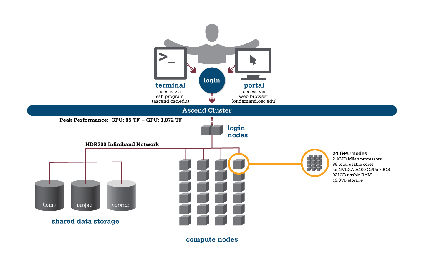
Hardware

Detailed system specifications:
- 24 Power Edge XE 8545 nodes, each with:
- 2 AMD EPYC 7643 (Milan) processors (2.3 GHz, each with 44 usable cores)
- 4 NVIDIA A100 GPUs with 80GB memory each, supercharged by NVIDIA NVLink
- 921GB usable RAM
- 12.8TB NVMe internal storage
- 2,112 total usable cores
- 88 cores/node & 921GB of memory/node
- Mellanox/NVIDA 200 Gbps HDR InfiniBand
- Theoretical system peak performance
- 1.95 petaflops
- 2 login nodes
- IP address: 192.148.247.[180-181]
How to Connect
-
SSH Method
To login to Ascend at OSC, ssh to the following hostname:
ascend.osc.edu
You can either use an ssh client application or execute ssh on the command line in a terminal window as follows:
ssh <username>@ascend.osc.edu
You may see a warning message including SSH key fingerprint. Verify that the fingerprint in the message matches one of the SSH key fingerprints listed here, then type yes.
From there, you are connected to the Ascend login node and have access to the compilers and other software development tools. You can run programs interactively or through batch requests. We use control groups on login nodes to keep the login nodes stable. Please use batch jobs for any compute-intensive or memory-intensive work. See the following sections for details.
-
OnDemand Method
You can also login to Ascend at OSC with our OnDemand tool. The first step is to log into OnDemand. Then once logged in you can access Ascend by clicking on "Clusters", and then selecting ">_Ascend Shell Access".
Instructions on how to connect to OnDemand can be found at the OnDemand documentation page.
File Systems
Ascend accesses the same OSC mass storage environment as our other clusters. Therefore, users have the same home directory as on the old clusters. Full details of the storage environment are available in our storage environment guide.
Software Environment
The module system on Ascend is the same as on the Owens and Pitzer systems. Use module load <package> to add a software package to your environment. Use module list to see what modules are currently loaded and module avail to see the modules that are available to load. To search for modules that may not be visible due to dependencies or conflicts, use module spider .
You can keep up to the software packages that have been made available on Ascend by viewing the Software by System page and selecting the Ascend system.
Batch Specifics
Refer to this Slurm migration page to understand how to use Slurm on the Ascend cluster.
Using OSC Resources
For more information about how to use OSC resources, please see our guide on batch processing at OSC. For specific information about modules and file storage, please see the Batch Execution Environment page.
Ascend Programming Environment
Compilers
C, C++ and Fortran are supported on the Ascend cluster. Intel, oneAPI, GNU, nvhpc, and aocc compiler suites are available. The Intel development tool chain is loaded by default. Compiler commands and recommended options for serial programs are listed in the table below. See also our compilation guide.
The Milan processors from AMD that make up Ascend support the Advanced Vector Extensions (AVX2) instruction set, but you must set the correct compiler flags to take advantage of it. AVX2 has the potential to speed up your code by a factor of 4 or more, depending on the compiler and options you would otherwise use. However, bare in mind that clock speeds decrease as the level of the instruction set increases. So, if your code does not benefit from vectorization it may be beneficial to use a lower instruction set.
In our experience, the Intel compiler usually does the best job of optimizing numerical codes and we recommend that you give it a try if you’ve been using another compiler.
With the Intel compilers, use -xHost and -O2 or higher. With the GNU compilers, use -march=native and -O3.
This advice assumes that you are building and running your code on Ascend. The executables will not be portable. Of course, any highly optimized builds, such as those employing the options above, should be thoroughly validated for correctness.
| LANGUAGE | INTEL | GNU |
|---|---|---|
| C | icc -O2 -xHost hello.c | gcc -O3 -march=native hello.c |
| Fortran 77/90 | ifort -O2 -xHost hello.F | gfortran -O3 -march=native hello.F |
| C++ | icpc -O2 -xHost hello.cpp | g++ -O3 -march=native hello.cpp |
Parallel Programming
MPI
OSC systems use the MVAPICH2 implementation of the Message Passing Interface (MPI), optimized for the high-speed Infiniband interconnect. MPI is a standard library for performing parallel processing using a distributed-memory model. For more information on building your MPI codes, please visit the MPI Library documentation.
MPI programs are started with the srun command. For example,
#!/bin/bash
#SBATCH --nodes=2
#SBATCH --ntasks-per-node=84
srun [ options ] mpi_prog
Note: the program to be run must either be in your path or have its path specified.
The srun command will normally spawn one MPI process per task requested in a Slurm batch job. Use the -n ntasks and/or --ntasks-per-node=n option to change that behavior. For example,
#!/bin/bash #SBATCH --nodes=2 # Use the maximum number of CPUs of two nodes srun ./mpi_prog # Run 8 processes per node srun -n 16 --ntasks-per-node=8 ./mpi_prog
The table below shows some commonly used options. Use srun -help for more information.
| OPTION | COMMENT |
|---|---|
-n, --ntasks=ntasks |
total number of tasks to run |
--ntasks-per-node=n |
number of tasks to invoke on each node |
-help |
Get a list of available options |
Note: The information above applies to the MVAPICH2, Intel MPI and OpenMPI installations at OSC.
Caution: mpiexec or mpirun is still supported with Intel MPI and OpenMPI, but it is not fully compatible in our Slurm environment. We recommand using
srun in any circumstances.OpenMP
The Intel, and GNU compilers understand the OpenMP set of directives, which support multithreaded programming. For more information on building OpenMP codes on OSC systems, please visit the OpenMP documentation.
An OpenMP program by default will use a number of threads equal to the number of CPUs requested in a Slurm batch job. To use a different number of threads, set the environment variable OMP_NUM_THREADS. For example,
#!/bin/bash #SBATCH --ntasks=8 # Run 8 threads ./omp_prog # Run 4 threads export OMP_NUM_THREADS=4 ./omp_prog
Interactive job only
Please use -c, --cpus-per-task=X instead of -n, --ntasks=X to request an interactive job. Both result in an interactive job with X CPUs available but only the former option automatically assigns the correct number of threads to the OpenMP program. If the option --ntasks is used only, the OpenMP program will use one thread or all threads will be bound to one CPU core.
Hybrid (MPI + OpenMP)
An example of running a job for hybrid code:
#!/bin/bash #SBATCH --nodes=2 #SBATCH --ntasks-per-node=80 # Run 4 MPI processes on each node and 40 OpenMP threads spawned from a MPI process export OMP_NUM_THREADS=40 srun -n 8 -c 40 --ntasks-per-node=4 ./hybrid_prog
Tuning Parallel Program Performance: Process/Thread Placement
To get the maximum performance, it is important to make sure that processes/threads are located as close as possible to their data, and as close as possible to each other if they need to work on the same piece of data, with given the arrangement of node, sockets, and cores, with different access to RAM and caches.
While cache and memory contention between threads/processes are an issue, it is best to use scatter distribution for code.
Processes and threads are placed differently depending on the computing resources you requste and the compiler and MPI implementation used to compile your code. For the former, see the above examples to learn how to run a job on exclusive nodes. For the latter, this section summarizes the default behavior and how to modify placement.
OpenMP only
For all two compilers (Intel, GNU), purely threaded codes do not bind to particular CPU cores by default. In other words, it is possible that multiple threads are bound to the same CPU core.
The following table describes how to modify the default placements for pure threaded code:
| DISTRIBUTION | Compact | Scatter/Cyclic |
|---|---|---|
| DESCRIPTION | Place threads close to each other as possible in successive order | Distribute threads as evenly as possible across sockets |
| INTEL | KMP_AFFINITY=compact | KMP_AFFINITY=scatter |
| GNU | OMP_PROC_BIND=true OMP_PLACE=cores |
OMP_PROC_BIND=true OMP_PLACE="{0},{48},{1},{49},..."[1] |
- The core IDs on the first and second sockets start with 0 and 48, respectively.
MPI Only
For MPI-only codes, MVAPICH2 first binds as many processes as possible on one socket, then allocates the remaining processes on the second socket so that consecutive tasks are near each other. Intel MPI and OpenMPI alternately bind processes on socket 1, socket 2, socket 1, socket 2 etc, as cyclic distribution.
For process distribution across nodes, all MPIs first bind as many processes as possible on one node, then allocates the remaining processes on the second node.
The following table describe how to modify the default placements on single node for MPI-only code with the command srun:
| DISTRIBUTION (single node) |
Compact | Scatter/Cyclic |
|---|---|---|
| DESCRIPTION | Place processs close to each other as possible in successive order | Distribute process as evenly as possible across sockets |
| MVAPICH2[1] | Default | MV2_CPU_BINDING_POLICY=scatter |
| INTEL MPI | srun --ntasks=84 --cpu-bind="map_cpu:$(seq -s, 0 43),$(seq -s, 48 95)" | Default |
| OPENMPI | srun --ntasks=84 --cpu-bind="map_cpu:$(seq -s, 0 43),$(seq -s, 48 95)" | Default |
MV2_CPU_BINDING_POLICYwill not work ifMV2_ENABLE_AFFINITY=0is set.
To distribute processes evenly across nodes, please set SLURM_DISTRIBUTION=cyclic.
Hybrid (MPI + OpenMP)
For Hybrid codes, each MPI process is allocated OMP_NUM_THREADS cores and the threads of each process are bound to those cores. All MPI processes (as well as the threads bound to the process) behave as we describe in the previous sections. It means the threads spawned from a MPI process might be bound to the same core. To change the default process/thread placmements, please refer to the tables above.
Summary
The above tables list the most commonly used settings for process/thread placement. Some compilers and Intel libraries may have additional options for process and thread placement beyond those mentioned on this page. For more information on a specific compiler/library, check the more detailed documentation for that library.
GPU Programming
96 NVIDIA A100 GPUs are available on Ascend. Please visit our GPU documentation.
Reference
Supercomputer:
Batch Limit Rules
We use Slurm syntax for all the discussions on this page. Please check how to prepare slurm job script if your script is prepared in PBS syntax.
Memory limit
It is strongly suggested to consider the memory use to the available per-core memory when users request OSC resources for their jobs.
Summary
| Node type | default memory per core (GB) | max usable memory per node (GB) |
|---|---|---|
| gpu (4 gpus) - 88 cores | 10.4726 GB | 921.5937 GB |
It is recommended to let the default memory apply unless more control over memory is needed.
Note that if an entire node is requested, then the job is automatically granted the entire node's main memory. On the other hand, if a partial node is requested, then memory is granted based on the default memory per core.
See a more detailed explanation below.
Default memory limits
A job can request resources and allow the default memory to apply. If a job requires 300 GB for example:
#SBATCH --ntasks=1 #SBATCH --cpus-per-task=30
This requests 30 cores, and each core will automatically be allocated 10.4 GB of memory (30 core * 10 GB memory = 300 GB memory).
Explicit memory requests
If needed, an explicit memory request can be added:
#SBATCH --ntasks=1 #SBATCH --cpus-per-task=4 #SBATCH --mem=300G
Job charging is determined either by number of cores or amount of memory.
See Job and storage charging for details.
See Job and storage charging for details.
CPU only jobs
Dense gpu nodes on Ascend have 88 cores each. However, cpuonly partition jobs may only request 84 cores per node.
An example request would look like:
#!/bin/bash #SBATCH --partition=cpuonly #SBATCH --time=5:00:00 #SBATCH --nodes=1 #SBATCH --ntasks=2 #SBATCH --cpus-per-task=42 # requests 2 tasks * 42 cores each = 84 cores <snip>
GPU Jobs
Jobs may request only parts of gpu node. These jobs may request up to the total cores on the node (88 cores).
Requests two gpus for one task:
#SBATCH --time=5:00:00 #SBATCH --nodes=1 #SBATCH --ntasks=1 #SBATCH --cpus-per-task=20 #SBATCH --gpus-per-task=2
Requests two gpus, one for each task:
#SBATCH --time=5:00:00 #SBATCH --nodes=1 #SBATCH --ntasks=2 #SBATCH --cpus-per-task=10 #SBATCH --gpus-per-task=1
Of course, jobs can request all the gpus of a dense gpu node as well. These jobs have access to all cores as well.
Request an entire dense gpu node:
#SBATCH --nodes=1 #SBATCH --ntasks=1 #SBATCH --cpus-per-task=88 #SBATCH --gpus-per-node=4
Partition time and job size limits
Here is the walltime and node limits per job for different queues/partitions available on Ascend:
|
NAME |
MAX TIME LIMIT |
MIN JOB SIZE |
MAX JOB SIZE |
NOTES |
|---|---|---|---|---|
|
cpuonly |
4-00:00:00 |
1 core |
4 nodes |
This partition may not request gpus 84 cores per node only |
| gpu |
7-00:00:00 |
1 core |
4 nodes |
|
| debug | 1:00:00 | 1 core | 2 nodes |
Usually, you do not need to specify the partition for a job and the scheduler will assign the right partition based on the requested resources. To specify a partition for a job, either add the flag --partition=<partition-name> to the sbatch command at submission time or add this line to the job script:#SBATCH --paritition=<partition-name>
Job/Core Limits
| Max Running Job Limit | Max Core/Processor Limit | Max GPU limit | ||
|---|---|---|---|---|
| For all types | GPU debug jobs | For all types | ||
| Individual User | 256 | 4 |
704 |
32 |
| Project/Group | 512 | n/a | 704 | 32 |
An individual user can have up to the max concurrently running jobs and/or up to the max processors/cores in use. However, among all the users in a particular group/project, they can have up to the max concurrently running jobs and/or up to the max processors/cores in use.
A user may have no more than 1000 jobs submitted to the parallel queue.
Supercomputer:
Service:
Migrating jobs from other clusters
This page includes a summary of differences to keep in mind when migrating jobs from other clusters to Ascend.
Guidance for Pitzer Users
Hardware Specifications
| Ascend (PER NODE) | Pitzer (PER NODE) | ||
|---|---|---|---|
| Regular compute node | n/a |
40 cores and 192GB of RAM 48 cores and 192GB of RAM |
|
| Huge memory node |
n/a |
48 cores and 768GB of RAM (12 nodes in this class) 80 cores and 3.0 TB of RAM (4 nodes in this class) |
|
| GPU Node |
88 cores and 921GB RAM 4 GPUs per node (24 nodes in this class) |
40 cores and 192GB of RAM, 2 GPUs per node (32 nodes in this class) 48 cores and 192GB of RAM, 2 GPUs per node (42 nodes in this class) |
|
Guidance for Owens Users
Hardware Specifications
| Ascend (PER NODE) | Owens (PER NODE) | ||
|---|---|---|---|
| Regular compute node | n/a | 28 cores and 125GB of RAM | |
| Huge memory node | n/a |
48 cores and 1.5TB of RAM (16 nodes in this class) |
|
| GPU node |
88 cores and 921GB RAM 4 GPUs per node (24 nodes in this class) |
28 cores and 125GB of RAM, 1 GPU per node (160 nodes in this class) |
|
File Systems
Ascend accesses the same OSC mass storage environment as our other clusters. Therefore, users have the same home directory, project space, and scratch space as on the other clusters.
Software Environment
Ascend uses the same module system as other OSC Clusters.
Use module load <package> to add a software package to your environment. Use module list to see what modules are currently loaded and module avail to see the modules that are available to load. To search for modules that may not be visible due to dependencies or conflicts, use module spider .
You can keep up to on the software packages that have been made available on Ascend by viewing the Software by System page and selecting the Ascend system.
Programming Environment
C, C++ and Fortran are supported on the Ascend cluster. Intel, oneAPI, GNU, nvhpc, and aocc compiler suites are available. The Intel development tool chain is loaded by default. To switch to a different compiler, use module swap . Ascend also uses the MVAPICH2 implementation of the Message Passing Interface (MPI).
See the Ascend Programming Environment page for details.
Supercomputer:
Service:
Ascend SSH key fingerprints
These are the public key fingerprints for Ascend:
ascend: ssh_host_rsa_key.pub = 2f:ad:ee:99:5a:f4:7f:0d:58:8f:d1:70:9d:e4:f4:16
ascend: ssh_host_ed25519_key.pub = 6b:0e:f1:fb:10:da:8c:0b:36:12:04:57:2b:2c:2b:4d
ascend: ssh_host_ecdsa_key.pub = f4:6f:b5:d2:fa:96:02:73:9a:40:5e:cf:ad:6d:19:e5
These are the SHA256 hashes:
ascend: ssh_host_rsa_key.pub = SHA256:4l25PJOI9sDUaz9NjUJ9z/GIiw0QV/h86DOoudzk4oQ
ascend: ssh_host_ed25519_key.pub = SHA256:pvz/XrtS+PPv4nsn6G10Nfc7yM7CtWoTnkgQwz+WmNY
ascend: ssh_host_ecdsa_key.pub = SHA256:giMUelxDSD8BTWwyECO10SCohi3ahLPBtkL2qJ3l080
Supercomputer:
Citation
For more information about citations of OSC, visit https://www.osc.edu/citation.
To cite Ascend, please use the following Archival Resource Key:
ark:/19495/hpc3ww9d
Please adjust this citation to fit the citation style guidelines required.
Ohio Supercomputer Center. 2022. Ascend Supercomputer. Columbus, OH: Ohio Supercomputer Center. http://osc.edu/ark:/19495/hpc3ww9d
Here is the citation in BibTeX format:
@misc{Ascend2022,
ark = {ark:/19495/hpc3ww9d},
url = {http://osc.edu/ark:/19495/hpc3ww9d},
year = {2022},
author = {Ohio Supercomputer Center},
title = {Ascend Supercomputer}
}
And in EndNote format:
%0 Generic %T Ascend Supercomputer %A Ohio Supercomputer Center %R ark:/19495/hpc3ww9d %U http://osc.edu/ark:/19495/hpc3ww9d %D 2022
Supercomputer:
Request access
Users who would like to use the Ascend cluster will need to request access. This is because of the particulars of the Ascend environment, which includes its size, GPUs, and scheduling policies.
Motivation
Access to Ascend is done on a case by case basis because:
- All nodes on Ascend are with 4 GPUs, and therefore it favors GPU work instead of CPU-only work
- It is a smaller machine than Pitzer and Owens, and thus has limited space for users
Good Ascend Workload Characteristics
Those interested in using Ascend should check that their work is well suited for it by using the following list. Ideal workloads will exhibit one or more of the following characteristics:
- Needs access to Ascend specific hardware (GPUs, or AMD)
- Software:
- Supports GPUs
- Takes advantage of:
- Long vector length
- Higher core count
- Improved memory bandwidth
Applying for Access
PIs of groups that would like to be considered for Ascend access should send the following in a email to OSC Help:
- Name
- Username
- Project code (group)
- Software/packages used on Ascend
- Evidence of workload being well suited for Ascend
Supercomputer:
Technical Specifications
The following are technical specifications for Ascend.
- Number of Nodes
-
24 nodes
- Number of CPU Sockets
-
48 (2 sockets/node)
- Number of CPU Cores
-
2,304 (96 cores/node)
- Cores Per Node
-
96 cores/node (88 usable cores/node)
- Internal Storage
-
12.8 TB NVMe internal storage
- Compute CPU Specifications
-
AMD EPYC 7643 (Milan) processors for compute
- 2.3 GHz
- 48 cores per processor
- Computer Server Specifications
-
24 Dell XE8545 servers
- Accelerator Specifications
-
4 NVIDIA A100 GPUs with 80GB memory each, supercharged by NVIDIA NVLink
- Number of Accelerator Nodes
-
24 total
- Total Memory
- ~ 24 TB
- Physical Memory Per Node
-
1 TB
- Physical Memory Per Core
-
10.6 GB
- Interconnect
-
Mellanox/NVIDA 200 Gbps HDR InfiniBand
Supercomputer:
Cardinal
OSC's Cardinal cluster is slated to launch in 2024.
Detailed system specifications:
-
378 Dell Nodes, 39,312 total cores, 128 GPUs
-
Dense Compute: 326 Dell PowerEdge C6620 two-socket servers, each with:
-
2 Intel Xeon CPU Max 9470 (Sapphire Rapids, 52 cores [48 usable], 2.0 GHz) processors
-
128 GB HBM2e and 512 GB DDR5 memory
-
1.6 TB NVMe local storage
-
NDR200 Infiniband
-
-
GPU Compute: 32 Dell PowerEdge XE9640 two-socket servers, each with:
-
2 Intel Xeon Platinum 8470 (Sapphire Rapids, 52 cores [48 usable], 2.0 GHz) processors
-
1 TB DDR5 memory
-
4 NVIDIA H100 (Hopper) GPUs each with 94 GB HBM2e memory and NVIDIA NVLink
-
12.8 TB NVMe local storage
-
Four NDR400 Infiniband HCAs supporting GPUDirect
-
-
Analytics: 16 Dell PowerEdge R660 two-socket servers, each with:
-
2 Intel Xeon CPU Max 9470 (Sapphire Rapids, 52 cores [48 usable], 2.0 GHz) processors
-
128 GB HBM2e and 2 TB DDR5 memory
-
12.8 TB NVMe local storage
-
NDR200 Infiniband
-
-
Login nodes: 4 Dell PowerEdge R660 two-socket servers, each with:
-
2 Intel Xeon CPU Max 9470 (Sapphire Rapids, 52 cores [48 usable], 2.0 GHz) processors
-
128 GB HBM and 1 TB DDR5 memory
-
3.2 TB NVMe local storage
-
NDR200 Infiniband
-
IP address: TBD
-
-
~10.5 PF Theoretical system peak performance
-
~8 PetaFLOPs (GPU)
-
~2.5 PetaFLOPS (CPU)
-
-
9 Physical racks, plus Two Coolant Distribution Units (CDUs) providing direct-to-the-chip liquid cooling for all nodes
Service:
Technical Specifications
The following are technical specifications for Cardinal.
- Number of Nodes
-
378 nodes
- Number of CPU Sockets
-
756 (2 sockets/node for all nodes)
- Number of CPU Cores
-
39,312
- Cores Per Node
-
104 cores/node for all nodes (96 usable)
- Local Disk Space Per Node
-
- 1.6 TB for compute nodes
- 12.8 TB for GPU and Large mem nodes
- 3.2 TB for login nodes
- Compute, Large Mem & Login Node CPU Specifications
- Intel Xeon CPU Max 9470 HBM2e (Sapphire Rapids)
- 2.0 GHz
- 52 cores per processor (48 usable)
- GPU Node CPU Specifications
- Intel Xeon Platinum 8470 (Sapphire Rapids)
- 2.0 GHz
- 52 cores per processor
- Server Specifications
-
- 326 Dell PowerEdge C6620
- 32 Dell PowerEdge XE9640 (GPU nodes)
- 20 Dell PowerEdge R660 (largemem & login nodes)
- Accelerator Specifications
-
NVIDIA H100 (Hopper) GPUs each with 96 GB HBM2e memory and NVIDIA NVLINK
- Number of Accelerator Nodes
-
32 quad GPU nodes (4 GPUs per node)
- Total Memory
-
~281 TB (44 TB HBM, 237 TB DDR5)
- Memory Per Node
-
- 128 GB HBM / 512 GB DDR5 (compute nodes)
- 1 TB (GPU nodes)
- 128 GB HBM / 2 TB DDR5 (large mem nodes)
- 128 GB HBM / 1 TB DDR5 (login nodes)
- Memory Per Core
-
- 1.2 GB HBM / 4.9 GB DDR5 (compute nodes)
- 9.8 GB (GPU nodes)
- 1.2 GB HBM / 19.7 GB DDR5 (large mem nodes)
- 1.2 GB HBM / 9.8 GB DDR5 (login nodes)
- Interconnect
-
- NDR200 Infiniband (200 Gbps) (compute, large mem, login nodes)
- 4x NDR400 Infiniband (400 Gbps x 4) with GPUDirect, allowing non-blocking communication between up to 10 nodes (GPU nodes)
Service:
Owens
TIP: Remember to check the menu to the right of the page for related pages with more information about Owens' specifics.
OSC's Owens cluster being installed in 2016 is a Dell-built, Intel® Xeon® processor-based supercomputer.
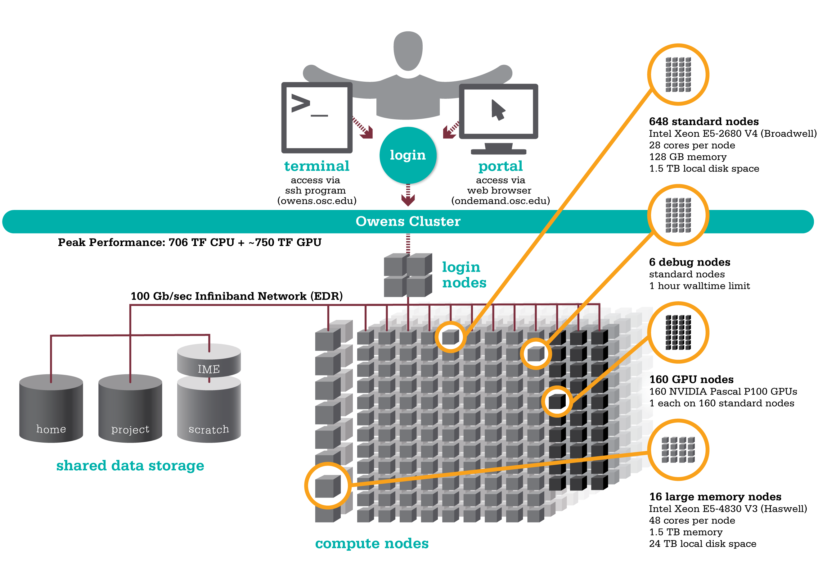 ,
,Hardware
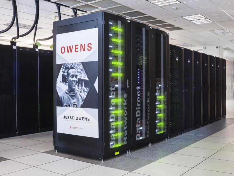
Detailed system specifications:
The memory information below is for total memory (RAM) on the node, however some amount of that is reserved for system use and not available to user processes.
Please see owens batch limits for details on user available memory amount.
Please see owens batch limits for details on user available memory amount.
- 824 Dell Nodes
- Dense Compute
-
648 compute nodes (Dell PowerEdge C6320 two-socket servers with Intel Xeon E5-2680 v4 (Broadwell, 14 cores, 2.40 GHz) processors, 128 GB memory)
-
-
GPU Compute
-
160 ‘GPU ready’ compute nodes -- Dell PowerEdge R730 two-socket servers with Intel Xeon E5-2680 v4 (Broadwell, 14 cores, 2.40 GHz) processors, 128 GB memory
-
NVIDIA Tesla P100 (Pascal) GPUs -- 5.3 TF peak (double precision), 16 GB memory
-
-
Analytics
-
16 huge memory nodes (Dell PowerEdge R930 four-socket server with Intel Xeon E5-4830 v3 (Haswell 12 core, 2.10 GHz) processors, 1,536 GB memory, 12 x 2 TB drives)
-
- 23,392 total cores
- 28 cores/node & 128 GB of memory/node
- Mellanox EDR (100 Gbps) Infiniband networking
- Theoretical system peak performance
- ~750 teraflops (CPU only)
- 4 login nodes:
- Intel Xeon E5-2680 (Broadwell) CPUs
- 28 cores/node and 256 GB of memory/node
- IP address: 192.148.247.[141-144]
How to Connect
-
SSH Method
To login to Owens at OSC, ssh to the following hostname:
owens.osc.edu
You can either use an ssh client application or execute ssh on the command line in a terminal window as follows:
ssh <username>@owens.osc.edu
You may see warning message including SSH key fingerprint. Verify that the fingerprint in the message matches one of the SSH key fingerprint listed here, then type yes.
From there, you are connected to Owens login node and have access to the compilers and other software development tools. You can run programs interactively or through batch requests. We use control groups on login nodes to keep the login nodes stable. Please use batch jobs for any compute-intensive or memory-intensive work. See the following sections for details.
-
OnDemand Method
You can also login to Owens at OSC with our OnDemand tool. The first step is to login to OnDemand. Then once logged in you can access Owens by clicking on "Clusters", and then selecting ">_Owens Shell Access".
Instructions on how to connect to OnDemand can be found at the OnDemand documention page.
File Systems
Owens accesses the same OSC mass storage environment as our other clusters. Therefore, users have the same home directory as on the old clusters. Full details of the storage environment are available in our storage environment guide.
Software Environment
The module system is used to manage the software environment on owens. Use module load <package> to add a software package to your environment. Use module list to see what modules are currently loaded and module avail to see the modules that are available to load. To search for modules that may not be visible due to dependencies or conflicts, use module spider . By default, you will have the batch scheduling software modules, the Intel compiler and an appropriate version of mvapich2 loaded.
You can keep up to on the software packages that have been made available on Owens by viewing the Software by System page and selecting the Owens system.
Compiling Code to Use Advanced Vector Extensions (AVX2)
The Haswell and Broadwell processors that make up Owens support the Advanced Vector Extensions (AVX2) instruction set, but you must set the correct compiler flags to take advantage of it. AVX2 has the potential to speed up your code by a factor of 4 or more, depending on the compiler and options you would otherwise use.
In our experience, the Intel and PGI compilers do a much better job than the gnu compilers at optimizing HPC code.
With the Intel compilers, use -xHost and -O2 or higher. With the gnu compilers, use -march=native and -O3 . The PGI compilers by default use the highest available instruction set, so no additional flags are necessary.
This advice assumes that you are building and running your code on Owens. The executables will not be portable. Of course, any highly optimized builds, such as those employing the options above, should be thoroughly validated for correctness.
See the Owens Programming Environment page for details.
Batch Specifics
Refer to the documentation for our batch environment to understand how to use the batch system on OSC hardware. Some specifics you will need to know to create well-formed batch scripts:
- Most compute nodes on Owens have 28 cores/processors per node. Huge-memory (analytics) nodes have 48 cores/processors per node.
- Jobs on Owens may request partial nodes.
Using OSC Resources
For more information about how to use OSC resources, please see our guide on batch processing at OSC. For specific information about modules and file storage, please see the Batch Execution Environment page.
Supercomputer:
Service:
Technical Specifications
The following are technical specifications for Owens.
- Number of Nodes
-
824 nodes
- Number of CPU Sockets
-
1,648 (2 sockets/node)
- Number of CPU Cores
-
23,392 (28 cores/node)
- Cores Per Node
-
28 cores/node (48 cores/node for Huge Mem Nodes)
- Local Disk Space Per Node
-
~1,500GB in /tmp
- Compute CPU Specifications
-
Intel Xeon E5-2680 v4 (Broadwell) for compute
- 2.4 GHz
- 14 cores per processor
- Computer Server Specifications
-
- 648 Dell PowerEdge C6320
- 160 Dell PowerEdge R730 (for accelerator nodes)
- Accelerator Specifications
-
NVIDIA P100 "Pascal" GPUs 16GB memory
- Number of Accelerator Nodes
-
160 total
- Total Memory
- ~ 127 TB
- Memory Per Node
-
128 GB (1.5 TB for Huge Mem Nodes)
- Memory Per Core
-
4.5 GB (31 GB for Huge Mem)
- Interconnect
-
Mellanox EDR Infiniband Networking (100Gbps)
- Login Specifications
-
4 Intel Xeon E5-2680 (Broadwell) CPUs
- 28 cores/node and 256GB of memory/node
- Special Nodes
-
16 Huge Memory Nodes
- Dell PowerEdge R930
- 4 Intel Xeon E5-4830 v3 (Haswell)
- 12 Cores
- 2.1 GHz
- 48 cores (12 cores/CPU)
- 1.5 TB Memory
- 12 x 2 TB Drive (20TB usable)
Supercomputer:
Service:
Environment changes in Slurm migration
As we migrate to Slurm from Torque/Moab, there will be necessary software environment changes.
Decommissioning old MVAPICH2 versions
Old MVAPICH2 including mvapich2/2.1, mvapich2/2.2 and its variants do not support Slurm very well due to its life span, so we will remove the following versions:
- mvapich2/2.1
- mvapich2/2.2, 2.2rc1, 2.2ddn1.3, 2.2ddn1.4, 2.2-debug, 2.2-gpu
As a result, the following dependent software will not be available anymore.
| Unavailable Software | Possible replacement |
|---|---|
| amber/16 | amber/18 |
| darshan/3.1.4 | darshan/3.1.6 |
| darshan/3.1.5-pre1 | darshan/3.1.6 |
| expresso/5.2.1 | expresso/6.3 |
| expresso/6.1 | expresso/6.3 |
| expresso/6.1.2 | expresso/6.3 |
| fftw3/3.3.4 | fftw3/3.3.5 |
| gamess/18Aug2016R1 | gamess/30Sep2019R2 |
| gromacs/2016.4 | gromacs/2018.2 |
| gromacs/5.1.2 | gromacs/2018.2 |
| lammps/14May16 | lammps/16Mar18 |
| lammps/31Mar17 | lammps/16Mar18 |
| mumps/5.0.2 | N/A (no current users) |
| namd/2.11 | namd/2.13 |
| nwchem/6.6 | nwchem/6.8 |
| pnetcdf/1.7.0 | pnetcdf/1.10.0 |
| siesta-par/4.0 | siesta-par/4.0.2 |
If you used one of the software listed above, we strongly recommend testing during the early user period. We listed a possible replacement version that is close to the unavailable version. However, if it is possible, we recommend using the most recent versions available. You can find the available versions by module spider {software name}. If you have any questions, please contact OSC Help.
Miscellaneous cleanup on MPIs
We clean up miscellaneous MPIs as we have a better and compatible version available. Since it has a compatible version, you should be able to use your applications without issues.
| Removed MPI versions | Compatible MPI versions |
|---|---|
|
mvapich2/2.3b mvapich2/2.3rc1 mvapich2/2.3rc2 |
mvapich2/2.3 mvapich2/2.3.3 |
|
mvapich2/2.3b-gpu mvapich2/2.3rc1-gpu mvapich2/2.3rc2-gpu mvapich2/2.3-gpu mvapich2/2.3.1-gpu mvapich2-gdr/2.3.1, 2.3.2, 2.3.3 |
mvapich2-gdr/2.3.4 |
|
openmpi/1.10.5 openmpi/1.10 |
openmpi/1.10.7 openmpi/1.10.7-hpcx |
|
openmpi/2.0 openmpi/2.0.3 openmpi/2.1.2 |
openmpi/2.1.6 openmpi/2.1.6-hpcx |
|
openmpi/4.0.2 openmpi/4.0.2-hpcx |
openmpi/4.0.3 openmpi/4.0.3-hpcx |
Software flag usage update for Licensed Software
We have software flags required to use in job scripts for licensed software, such as ansys, abauqs, or schrodinger. With the slurm migration, we updated the syntax and added extra software flags. It is very important everyone follow the procedure below. If you don't use the software flags properly, jobs submitted by others can be affected.
We require using software flags only for the demanding software and the software features in order to prevent job failures due to insufficient licenses. When you use the software flags, Slurm will record it on its license pool, so that other jobs will launch when there are enough licenses available. This will function correctly when everyone uses the software flag.
During the early user period until Dec 15, 2020, the software flag system may not work correctly. This is because, during the test period, licenses will be used from two separate Owens systems. However, we recommend you to test your job scripts with the new software flags, so that you can use it without any issues after the slurm migration.
The new syntax for software flags is
#SBATCH -L {software flag}@osc:N
where N is the requesting number of the licenses. If you need more than one software flags, you can use
#SBATCH -L {software flag1}@osc:N,{software flag2}@osc:M
For example, if you need 2 abaqus and 2 abaqusextended license features, then you can use
$SBATCH -L abaqus@osc:2,abaqusextended@osc:2
We have the full list of software associated with software flags in the table below.
| Software flag | Note | |
|---|---|---|
| abaqus |
abaqus, abaquscae |
|
| ansys | ansys, ansyspar | |
| comsol | comsolscript | |
| schrodinger | epik, glide, ligprep, macromodel, qikprop | |
| starccm | starccm, starccmpar | |
| stata | stata | |
| usearch | usearch | |
| ls-dyna, mpp-dyna | lsdyna |
Supercomputer:
Service:
Owens Programming Environment (PBS)
This document is obsoleted and kept as a reference to previous Owens programming environment. Please refer to here for the latest version.
Compilers
C, C++ and Fortran are supported on the Owens cluster. Intel, PGI and GNU compiler suites are available. The Intel development tool chain is loaded by default. Compiler commands and recommended options for serial programs are listed in the table below. See also our compilation guide.
The Haswell and Broadwell processors that make up Owens support the Advanced Vector Extensions (AVX2) instruction set, but you must set the correct compiler flags to take advantage of it. AVX2 has the potential to speed up your code by a factor of 4 or more, depending on the compiler and options you would otherwise use.
In our experience, the Intel and PGI compilers do a much better job than the GNU compilers at optimizing HPC code.
With the Intel compilers, use -xHost and -O2 or higher. With the GNU compilers, use -march=native and -O3. The PGI compilers by default use the highest available instruction set, so no additional flags are necessary.
This advice assumes that you are building and running your code on Owens. The executables will not be portable. Of course, any highly optimized builds, such as those employing the options above, should be thoroughly validated for correctness.
| LANGUAGE | INTEL EXAMPLE | PGI EXAMPLE | GNU EXAMPLE |
|---|---|---|---|
| C | icc -O2 -xHost hello.c | pgcc -fast hello.c | gcc -O3 -march=native hello.c |
| Fortran 90 | ifort -O2 -xHost hello.f90 | pgf90 -fast hello.f90 | gfortran -O3 -march=native hello.f90 |
| C++ | icpc -O2 -xHost hello.cpp | pgc++ -fast hello.cpp | g++ -O3 -march=native hello.cpp |
Parallel Programming
MPI
OSC systems use the MVAPICH2 implementation of the Message Passing Interface (MPI), optimized for the high-speed Infiniband interconnect. MPI is a standard library for performing parallel processing using a distributed-memory model. For more information on building your MPI codes, please visit the MPI Library documentation.
Parallel programs are started with the mpiexec command. For example,
mpiexec ./myprog
The program to be run must either be in your path or have its path specified.
The mpiexec command will normally spawn one MPI process per CPU core requested in a batch job. Use the -n and/or -ppn option to change that behavior.
The table below shows some commonly used options. Use mpiexec -help for more information.
| MPIEXEC Option | COMMENT |
|---|---|
-ppn 1 |
One process per node |
-ppn procs |
procs processes per node |
-n totalprocs-np totalprocs |
At most totalprocs processes per node |
-prepend-rank |
Prepend rank to output |
-help |
Get a list of available options |
Caution: There are many variations on mpiexec and mpiexec.hydra. Information found on non-OSC websites may not be applicable to our installation.
The information above applies to the MVAPICH2 and IntelMPI installations at OSC. See the OpenMPI software page for mpiexec usage with OpenMPI.
OpenMP
The Intel, PGI and GNU compilers understand the OpenMP set of directives, which support multithreaded programming. For more information on building OpenMP codes on OSC systems, please visit the OpenMP documentation.
GPU Programming
160 Nvidia P100 GPUs are available on Owens. Please visit our GPU documentation.
Supercomputer:
Service:
Technologies:
Owens Programming Environment
Compilers
C, C++ and Fortran are supported on the Owens cluster. Intel, PGI and GNU compiler suites are available. The Intel development tool chain is loaded by default. Compiler commands and recommended options for serial programs are listed in the table below. See also our compilation guide.
The Haswell and Broadwell processors that make up Owens support the Advanced Vector Extensions (AVX2) instruction set, but you must set the correct compiler flags to take advantage of it. AVX2 has the potential to speed up your code by a factor of 4 or more, depending on the compiler and options you would otherwise use.
In our experience, the Intel and PGI compilers do a much better job than the GNU compilers at optimizing HPC code.
With the Intel compilers, use -xHost and -O2 or higher. With the GNU compilers, use -march=native and -O3. The PGI compilers by default use the highest available instruction set, so no additional flags are necessary.
This advice assumes that you are building and running your code on Owens. The executables will not be portable. Of course, any highly optimized builds, such as those employing the options above, should be thoroughly validated for correctness.
| LANGUAGE | INTEL | GNU | PGI |
|---|---|---|---|
| C | icc -O2 -xHost hello.c | gcc -O3 -march=native hello.c | pgcc -fast hello.c |
| Fortran 77/90 | ifort -O2 -xHost hello.F | gfortran -O3 -march=native hello.F | pgfortran -fast hello.F |
| C++ | icpc -O2 -xHost hello.cpp | g++ -O3 -march=native hello.cpp | pgc++ -fast hello.cpp |
Parallel Programming
MPI
OSC systems use the MVAPICH2 implementation of the Message Passing Interface (MPI), optimized for the high-speed Infiniband interconnect. MPI is a standard library for performing parallel processing using a distributed-memory model. For more information on building your MPI codes, please visit the MPI Library documentation.
MPI programs are started with the srun command. For example,
#!/bin/bash
#SBATCH --nodes=2
srun [ options ] mpi_prog
Note: the program to be run must either be in your path or have its path specified.
The srun command will normally spawn one MPI process per task requested in a Slurm batch job. Use the -n ntasks and/or --ntasks-per-node=n option to change that behavior. For example,
#!/bin/bash #SBATCH --nodes=2 # Use the maximum number of CPUs of two nodes srun ./mpi_prog # Run 8 processes per node srun -n 16 --ntasks-per-node=8 ./mpi_prog
The table below shows some commonly used options. Use srun -help for more information.
| OPTION | COMMENT |
|---|---|
-n, --ntasks=ntasks |
total number of tasks to run |
--ntasks-per-node=n |
number of tasks to invoke on each node |
-help |
Get a list of available options |
Note: The information above applies to the MVAPICH2, Intel MPI and OpenMPI installations at OSC.
Caution: mpiexec or mpiexec.hydra is still supported with Intel MPI and OpenMPI, but it is not fully compatible in our Slurm environment. We recommand using
srun in any circumstances.OpenMP
The Intel, GNU and PGI compilers understand the OpenMP set of directives, which support multithreaded programming. For more information on building OpenMP codes on OSC systems, please visit the OpenMP documentation.
An OpenMP program by default will use a number of threads equal to the number of CPUs requested in a Slurm batch job. To use a different number of threads, set the environment variable OMP_NUM_THREADS. For example,
#!/bin/bash #SBATCH --ntasks=8 # Run 8 threads ./omp_prog # Run 4 threads export OMP_NUM_THREADS=4 ./omp_prog
To run a OpenMP job on an exclusive node:
#!/bin/bash #SBATCH --nodes=1 #SBATCH --exclusive export OMP_NUM_THREADS=$SLURM_CPUS_ON_NODE ./omp_prog
Interactive job only
See the section on interactive batch in batch job submission for details on submitting an interactive job to the cluster.
Hybrid (MPI + OpenMP)
An example of running a job for hybrid code:
#!/bin/bash #SBATCH --nodes=2 # Run 4 MPI processes on each node and 7 OpenMP threads spawned from a MPI process export OMP_NUM_THREADS=7 srun -n 8 -c 7 --ntasks-per-node=4 ./hybrid_prog
Tuning Parallel Program Performance: Process/Thread Placement
To get the maximum performance, it is important to make sure that processes/threads are located as close as possible to their data, and as close as possible to each other if they need to work on the same piece of data, with given the arrangement of node, sockets, and cores, with different access to RAM and caches.
While cache and memory contention between threads/processes are an issue, it is best to use scatter distribution for code.
Processes and threads are placed differently depending on the computing resources you requste and the compiler and MPI implementation used to compile your code. For the former, see the above examples to learn how to run a job on exclusive nodes. For the latter, this section summarizes the default behavior and how to modify placement.
OpenMP only
For all three compilers (Intel, GNU, PGI), purely threaded codes do not bind to particular CPU cores by default. In other words, it is possible that multiple threads are bound to the same CPU core.
The following table describes how to modify the default placements for pure threaded code:
| DISTRIBUTION | Compact | Scatter/Cyclic |
|---|---|---|
| DESCRIPTION | Place threads as closely as possible on sockets | Distribute threads as evenly as possible across sockets |
| INTEL | KMP_AFFINITY=compact | KMP_AFFINITY=scatter |
| GNU | OMP_PLACES=sockets[1] | OMP_PROC_BIND=spread/close |
| PGI[2] |
MP_BIND=yes |
MP_BIND=yes |
- Threads in the same socket might be bound to the same CPU core.
- PGI LLVM-backend (version 19.1 and later) does not support thread/processors affinity on NUMA architecture. To enable this feature, compile threaded code with
--Mnollvmto use proprietary backend.
MPI Only
For MPI-only codes, MVAPICH2 first binds as many processes as possible on one socket, then allocates the remaining processes on the second socket so that consecutive tasks are near each other. Intel MPI and OpenMPI alternately bind processes on socket 1, socket 2, socket 1, socket 2 etc, as cyclic distribution.
For process distribution across nodes, all MPIs first bind as many processes as possible on one node, then allocates the remaining processes on the second node.
The following table describe how to modify the default placements on a single node for MPI-only code with the command srun:
| DISTRIBUTION (single node) |
Compact | Scatter/Cyclic |
|---|---|---|
| DESCRIPTION | Place processs as closely as possible on sockets | Distribute process as evenly as possible across sockets |
| MVAPICH2[1] | Default | MV2_CPU_BINDING_POLICY=scatter |
| INTEL MPI | srun --cpu-bind="map_cpu:$(seq -s, 0 2 27),$(seq -s, 1 2 27)" | Default |
| OPENMPI | srun --cpu-bind="map_cpu:$(seq -s, 0 2 27),$(seq -s, 1 2 27)" | Default |
MV2_CPU_BINDING_POLICYwill not work ifMV2_ENABLE_AFFINITY=0is set.
To distribute processes evenly across nodes, please set SLURM_DISTRIBUTION=cyclic.
Hybrid (MPI + OpenMP)
For Hybrid codes, each MPI process is allocated OMP_NUM_THREADS cores and the threads of each process are bound to those cores. All MPI processes (as well as the threads bound to the process) behave as we describe in the previous sections. It means the threads spawned from a MPI process might be bound to the same core. To change the default process/thread placmements, please refer to the tables above.
Summary
The above tables list the most commonly used settings for process/thread placement. Some compilers and Intel libraries may have additional options for process and thread placement beyond those mentioned on this page. For more information on a specific compiler/library, check the more detailed documentation for that library.
GPU Programming
160 Nvidia P100 GPUs are available on Owens. Please visit our GPU documentation.
Reference
Supercomputer:
Service:
Technologies:
Citation
For more information about citations of OSC, visit https://www.osc.edu/citation.
To cite Owens, please use the following Archival Resource Key:
ark:/19495/hpc6h5b1
Please adjust this citation to fit the citation style guidelines required.
Ohio Supercomputer Center. 2016. Owens Supercomputer. Columbus, OH: Ohio Supercomputer Center. http://osc.edu/ark:19495/hpc6h5b1
Here is the citation in BibTeX format:
@misc{Owens2016,
ark = {ark:/19495/hpc93fc8},
url = {http://osc.edu/ark:/19495/hpc6h5b1},
year = {2016},
author = {Ohio Supercomputer Center},
title = {Owens Supercomputer}
}
And in EndNote format:
%0 Generic %T Owens Supercomputer %A Ohio Supercomputer Center %R ark:/19495/hpc6h5b1 %U http://osc.edu/ark:/19495/hpc6h5b1 %D 2016
Here is an .ris file to better suit your needs. Please change the import option to .ris.
Documentation Attachment:
Supercomputer:
Service:
Owens SSH key fingerprints
These are the public key fingerprints for Owens:
owens: ssh_host_rsa_key.pub = 18:68:d4:b0:44:a8:e2:74:59:cc:c8:e3:3a:fa:a5:3f
owens: ssh_host_ed25519_key.pub = 1c:3d:f9:99:79:06:ac:6e:3a:4b:26:81:69:1a:ce:83
owens: ssh_host_ecdsa_key.pub = d6:92:d1:b0:eb:bc:18:86:0c:df:c5:48:29:71:24:af
These are the SHA256 hashes:
owens: ssh_host_rsa_key.pub = SHA256:vYIOstM2e8xp7WDy5Dua1pt/FxmMJEsHtubqEowOaxo
owens: ssh_host_ed25519_key.pub = SHA256:FSb9ZxUoj5biXhAX85tcJ/+OmTnyFenaSy5ynkRIgV8
owens: ssh_host_ecdsa_key.pub = SHA256:+fqAIqaMW/DUJDB0v/FTxMT9rkbvi/qVdMKVROHmAP4
Supercomputer:
Batch Limit Rules
Memory Limit:
A small portion of the total physical memory on each node is reserved for distributed processes. The actual physical memory available to user jobs is tabulated below.
Summary
| Node type | default and max memory per core | max memory per node |
|---|---|---|
| regular compute | 4.214 GB | 117 GB |
| huge memory | 31.104 GB | 1492 GB |
| gpu | 4.214 GB | 117 GB |
A job may request more than the max memory per core, but the job will be allocated more cores to satisfy the memory request instead of just more memory.
e.g. The following slurm directives will actually grant this job 3 cores, with 10 GB of memory
(since 2 cores * 4.2 GB = 8.4 GB doesn't satisfy the memory request).
e.g. The following slurm directives will actually grant this job 3 cores, with 10 GB of memory
(since 2 cores * 4.2 GB = 8.4 GB doesn't satisfy the memory request).
#SBATCH --ntask=2
#SBATCH --mem=10gIt is recommended to let the default memory apply unless more control over memory is needed.
Note that if an entire node is requested, then the job is automatically granted the entire node's main memory. On the other hand, if a partial node is requested, then memory is granted based on the default memory per core.
See a more detailed explanation below.
Regular Dense Compute Node
On Owens, it equates to 4,315 MB/core or 120,820 MB/node (117.98 GB/node) for the regular dense compute node.
If your job requests less than a full node ( ntasks< 28 ), it may be scheduled on a node with other running jobs. In this case, your job is entitled to a memory allocation proportional to the number of cores requested (4315 MB/core). For example, without any memory request ( mem=XXMB ), a job that requests --nodes=1 --ntasks=1 will be assigned one core and should use no more than 4315 MB of RAM, a job that requests --nodes=1 --ntasks=3 will be assigned 3 cores and should use no more than 3*4315 MB of RAM, and a job that requests --nodes=1 --ntasks=28 will be assigned the whole node (28 cores) with 118 GB of RAM.
Here is some information when you include memory request (mem=XX ) in your job. A job that requests --nodes=1 --ntasks=1 --mem=12GB will be assigned three cores and have access to 12 GB of RAM, and charged for 3 cores worth of usage (in other ways, the request --ntasks is ingored). A job that requests --nodes=1 --ntasks=5 --mem=12GB will be assigned 5 cores but have access to only 12 GB of RAM, and charged for 5 cores worth of usage.
A multi-node job ( nodes>1 ) will be assigned the entire nodes with 118 GB/node and charged for the entire nodes regardless of ppn request. For example, a job that requests --nodes=10 --ntasks-per-node=1 will be charged for 10 whole nodes (28 cores/node*10 nodes, which is 280 cores worth of usage).
Huge Memory Node
Beginning on Tuesday, March 10th, 2020, users are able to run jobs using less than a full huge memory node. Please read the following instructions carefully before requesting a huge memory node on Owens.
On Owens, it equates to 31,850 MB/core or 1,528,800 MB/node (1,492.96 GB/node) for a huge memory node.
To request no more than a full huge memory node, you have two options:
- The first is to specify the memory request between 120,832 MB (118 GB) and 1,528,800 MB (1,492.96 GB), i.e.,
120832MB <= mem <=1528800MB(118GB <= mem < 1493GB). Note: you can only use interger for request - The other option is to use the combination of
--ntasks-per-nodeand--partition, like--ntasks-per-node=4 --partition=hugemem. When no memory is specified for the huge memory node, your job is entitled to a memory allocation proportional to the number of cores requested (31,850MB/core). Note,--ntasks-per-nodeshould be no less than 4 and no more than 48.
To manage and monitor your memory usage, please refer to Out-of-Memory (OOM) or Excessive Memory Usage.
GPU Jobs
There is only one GPU per GPU node on Owens.
For serial jobs, we allow node sharing on GPU nodes so a job may request any number of cores (up to 28)
(--nodes=1 --ntasks=XX --gpus-per-node=1)
For parallel jobs (n>1), we do not allow node sharing.
See this GPU computing page for more information.
Partition time and job size limits
Here are the partitions available on Owens:
| Name | Max time limit (dd-hh:mm:ss) |
Min job size | Max job size | notes |
|---|---|---|---|---|
|
serial |
7-00:00:00 |
1 core |
1 node |
|
|
longserial |
14-00:00:0 |
1 core |
1 node |
|
|
parallel |
4-00:00:00 |
2 nodes |
81 nodes |
|
| gpuserial | 7-00:00:00 | 1 core | 1 node | |
| gpuparallel | 4-00:00:00 | 2 nodes | 8 nodes | |
|
hugemem |
7-00:00:00 |
1 core |
1 node |
|
| hugemem-parallel | 4-00:00:00 | 2 nodes | 16 nodes |
|
| debug | 1:00:00 | 1 core | 2 nodes |
|
| gpudebug | 1:00:00 | 1 core | 2 nodes |
|
To specify a partition for a job, either add the flag
--partition=<partition-name> to the sbatch command at submission time or add this line to the job script:#SBATCH --paritition=<partition-name>To access one of the restricted queues, please contact OSC Help. Generally, access will only be granted to these queues if the performance of the job cannot be improved, and job size cannot be reduced by splitting or checkpointing the job.
Job/Core Limits
| Max Running Job Limit | Max Core/Processor Limit | ||||
|---|---|---|---|---|---|
| For all types | GPU jobs | Regular debug jobs | GPU debug jobs | For all types | |
| Individual User | 384 | 132 | 4 | 4 | 3080 |
| Project/Group | 576 | 132 | n/a | n/a | 3080 |
An individual user can have up to the max concurrently running jobs and/or up to the max processors/cores in use.
However, among all the users in a particular group/project, they can have up to the max concurrently running jobs and/or up to the max processors/cores in use.
A user may have no more than 1000 jobs submitted to both the parallel and serial job queue separately.
Supercomputer:
Service:
Pitzer
TIP: Remember to check the menu to the right of the page for related pages with more information about Pitzer's specifics.
OSC's original Pitzer cluster was installed in late 2018 and is a Dell-built, Intel® Xeon® 'Skylake' processor-based supercomputer with 260 nodes.
In September 2020, OSC installed additional 398 Intel® Xeon® 'Cascade Lake' processor-based nodes as part of a Pitzer Expansion cluster.
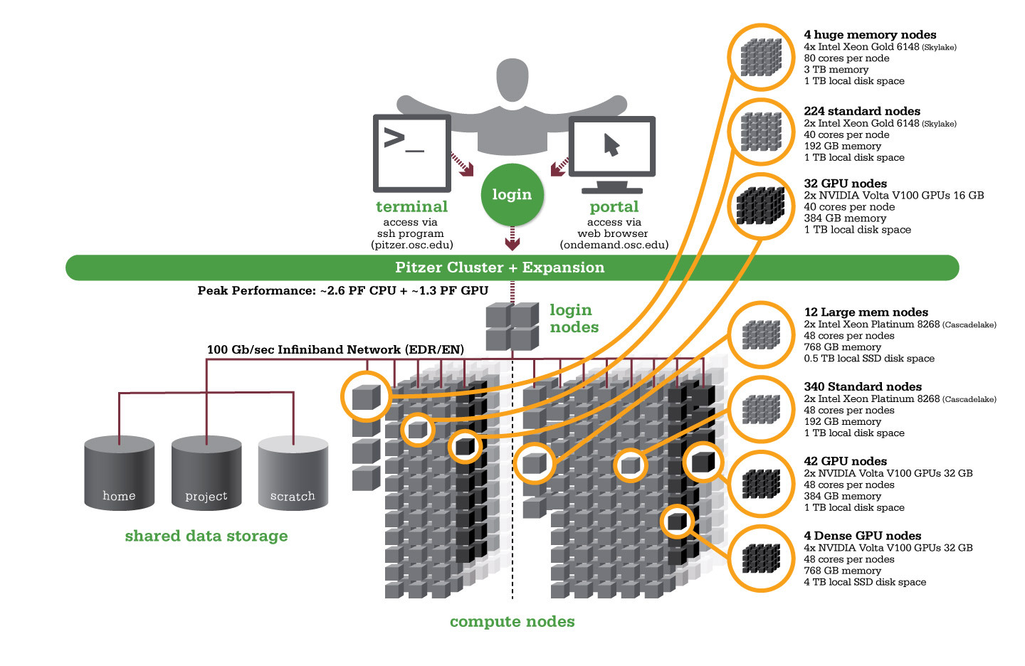
Hardware

Detailed system specifications:
| Deployed in 2018 | Deployed in 2020 | Total | |
|---|---|---|---|
| Total Compute Nodes | 260 Dell nodes | 398 Dell nodes | 658 Dell nodes |
| Total CPU Cores | 10,560 total cores | 19,104 total cores | 29,664 total cores |
| Standard Dense Compute Nodes |
224 nodes
|
340 nodes
|
564 nodes |
| Dual GPU Compute Nodes | 32 nodes
|
42 nodes
|
74 dual GPU nodes |
| Quad GPU Compute Nodes | N/A | 4 nodes
|
4 quad GPU nodes |
| Large Memory Compute Nodes | 4 nodes
|
12 nodes
|
16 nodes |
| Interactive Login Nodes |
4 nodes
|
4 nodes | |
| InfiniBand High-Speed Network | Mellanox EDR (100 Gbps) Infiniband networking | Mellanox EDR (100 Gbps) Infiniband networking | |
| Theoretical Peak Performance |
~850 TFLOPS (CPU only) ~450 TFLOPS (GPU only) ~1300 TFLOPS (total) |
~1900 TFLOPS (CPU only) ~700 TFLOPS (GPU only) ~2600 TFLOPS (total) |
~2750 TFLOPS (CPU only) ~1150 TFLOPS (GPU only) ~3900 TFLOPS (total) |
How to Connect
-
SSH Method
To login to Pitzer at OSC, ssh to the following hostname:
pitzer.osc.edu
You can either use an ssh client application or execute ssh on the command line in a terminal window as follows:
ssh <username>@pitzer.osc.edu
You may see a warning message including SSH key fingerprint. Verify that the fingerprint in the message matches one of the SSH key fingerprints listed here, then type yes.
From there, you are connected to the Pitzer login node and have access to the compilers and other software development tools. You can run programs interactively or through batch requests. We use control groups on login nodes to keep the login nodes stable. Please use batch jobs for any compute-intensive or memory-intensive work. See the following sections for details.
-
OnDemand Method
You can also login to Pitzer at OSC with our OnDemand tool. The first step is to log into OnDemand. Then once logged in you can access Pitzer by clicking on "Clusters", and then selecting ">_Pitzer Shell Access".
Instructions on how to connect to OnDemand can be found at the OnDemand documentation page.
File Systems
Pitzer accesses the same OSC mass storage environment as our other clusters. Therefore, users have the same home directory as on the old clusters. Full details of the storage environment are available in our storage environment guide.
Software Environment
The module system on Pitzer is the same as on the Owens and Ruby systems. Use module load <package> to add a software package to your environment. Use module list to see what modules are currently loaded and module avail to see the modules that are available to load. To search for modules that may not be visible due to dependencies or conflicts, use module spider . By default, you will have the batch scheduling software modules, the Intel compiler, and an appropriate version of mvapich2 loaded.
You can keep up to the software packages that have been made available on Pitzer by viewing the Software by System page and selecting the Pitzer system.
Compiling Code to Use Advanced Vector Extensions (AVX2)
The Skylake processors that make Pitzer support the Advanced Vector Extensions (AVX2) instruction set, but you must set the correct compiler flags to take advantage of it. AVX2 has the potential to speed up your code by a factor of 4 or more, depending on the compiler and options you would otherwise use.
In our experience, the Intel and PGI compilers do a much better job than the gnu compilers at optimizing HPC code.
With the Intel compilers, use -xHost and -O2 or higher. With the gnu compilers, use -march=native and -O3 . The PGI compilers by default use the highest available instruction set, so no additional flags are necessary.
This advice assumes that you are building and running your code on Pitzer. The executables will not be portable. Of course, any highly optimized builds, such as those employing the options above, should be thoroughly validated for correctness.
See the Pitzer Programming Environment page for details.
Batch Specifics
On September 22, 2020, OSC switches to Slurm for job scheduling and resource management on the Pitzer Cluster.
Refer to this Slurm migration page to understand how to use Slurm on the Pitzer cluster. Some specifics you will need to know to create well-formed batch scripts:
- OSC enables PBS compatibility layer provided by Slurm such that PBS batch scripts that used to work in the previous Torque/Moab environment mostly still work in Slurm.
- Pitzer is a heterogeneous system with mixed types of CPUs after the expansion as shown in the above table. Please be cautious when requesting resources on Pitzer and check this page for more detailed discussions
- Jobs on Pitzer may request partial nodes.
Using OSC Resources
For more information about how to use OSC resources, please see our guide on batch processing at OSC and Slurm migration. For specific information about modules and file storage, please see the Batch Execution Environment page.
Technical Specifications
- Login Specifications
-
4 Intel Xeon Gold 6148 (Skylake) CPUs
- 40 cores/node and 384 GB of memory/node
Technical specifications for 2018 Pitzer:
- Number of Nodes
-
260 nodes
- Number of CPU Sockets
-
528 (2 sockets/node for standard node)
- Number of CPU Cores
-
10,560 (40 cores/node for standard node)
- Cores Per Node
-
40 cores/node (80 cores/node for Huge Mem Nodes)
- Local Disk Space Per Node
-
850 GB in /tmp
- Compute CPU Specifications
-
Intel Xeon Gold 6148 (Skylake) for compute
- 2.4 GHz
- 20 cores per processor
- Computer Server Specifications
-
- 224 Dell PowerEdge C6420
- 32 Dell PowerEdge R740 (for accelerator nodes)
- 4 Dell PowerEdge R940
- Accelerator Specifications
-
NVIDIA V100 "Volta" GPUs 16GB memory
- Number of Accelerator Nodes
-
32 total (2 GPUs per node)
- Total Memory
-
~67 TB
- Memory Per Node
-
- 192 GB for standard nodes
- 384 GB for accelerator nodes
- 3 TB for Huge Mem Nodes
- Memory Per Core
-
- 4.8 GB for standard nodes
- 9.6 GB for accelerator nodes
- 76.8 GB for Huge Mem
- Interconnect
-
Mellanox EDR Infiniband Networking (100Gbps)
-
- Special Nodes
-
4 Huge Memory Nodes
- Dell PowerEdge R940
- 4 Intel Xeon Gold 6148 (Skylake)
- 20 Cores
- 2.4 GHz
- 80 cores (20 cores/CPU)
- 3 TB Memory
- 2x Mirror 1 TB Drive (1 TB usable)
Technical specifications for 2020 Pitzer:
- Number of Nodes
-
398 nodes
- Number of CPU Sockets
-
796 (2 sockets/node for all nodes)
- Number of CPU Cores
-
19,104 (48 cores/node for all nodes)
- Cores Per Node
-
48 cores/node for all nodes
- Local Disk Space Per Node
-
- 1 TB for most nodes
- 4 TB for quad GPU
- 0.5 TB for large mem
- Compute CPU Specifications
-
Intel Xeon 8268s Cascade Lakes for most compute
- 2.9 GHz
- 24 cores per processor
- Computer Server Specifications
-
- 352 Dell PowerEdge C6420
- 42 Dell PowerEdge R740 (for dual GPU nodes)
- 4 Dell Poweredge c4140 (for quad GPU nodes)
- Accelerator Specifications
-
- NVIDIA V100 "Volta" GPUs 32GB memory for dual GPU
- NVIDIA V100 "Volta" GPUs 32GB memory and NVLink for quad GPU
- Number of Accelerator Nodes
-
- 42 dual GPU nodes (2 GPUs per node)
- 4 quad GPU nodes (4 GPUs per node)
- Total Memory
-
~95 TB
- Memory Per Node
-
- 192 GB for standard nodes
- 384 GB for dual GPU nodes
- 768 GB for quad and Large Mem Nodes
- Memory Per Core
-
- 4.0 GB for standard nodes
- 8.0 GB for dual GPU nodes
- 16.0 GB for quad and Large Mem Nodes
- Interconnect
-
Mellanox EDR Infiniband Networking (100Gbps)
- Special Nodes
-
4 quad GPU Nodes
- Dual Intel Xeon 8260s Cascade Lakes
- Quad NVIDIA Volta V100s w/32GB GPU memory and NVLink
- 48 cores per node @ 2.4GHz
- 768GB memory
- 4 TB disk space
12 Large Memory Nodes- Dual Intel Xeon 8268 Cascade Lakes
- 48 cores per node @ 2.9GHz
- 768GB memory
- 0.5 TB disk space
Supercomputer:
Pitzer Programming Environment (PBS)
This document is obsoleted and kept as a reference to previous Pitzer programming environment. Please refer to here for the latest version.
Compilers
C, C++ and Fortran are supported on the Pitzer cluster. Intel, PGI and GNU compiler suites are available. The Intel development tool chain is loaded by default. Compiler commands and recommended options for serial programs are listed in the table below. See also our compilation guide.
The Skylake processors that make up Pitzer support the Advanced Vector Extensions (AVX512) instruction set, but you must set the correct compiler flags to take advantage of it. AVX512 has the potential to speed up your code by a factor of 8 or more, depending on the compiler and options you would otherwise use. However, bare in mind that clock speeds decrease as the level of the instruction set increases. So, if your code does not benefit from vectorization it may be beneficial to use a lower instruction set.
In our experience, the Intel and PGI compilers do a much better job than the GNU compilers at optimizing HPC code.
With the Intel compilers, use -xHost and -O2 or higher. With the GNU compilers, use -march=native and -O3. The PGI compilers by default use the highest available instruction set, so no additional flags are necessary.
This advice assumes that you are building and running your code on Owens. The executables will not be portable. Of course, any highly optimized builds, such as those employing the options above, should be thoroughly validated for correctness.
| LANGUAGE | INTEL EXAMPLE | PGI EXAMPLE | GNU EXAMPLE |
|---|---|---|---|
| C | icc -O2 -xHost hello.c | pgcc -fast hello.c | gcc -O3 -march=native hello.c |
| Fortran 90 | ifort -O2 -xHost hello.f90 | pgf90 -fast hello.f90 | gfortran -O3 -march=native hello.f90 |
| C++ | icpc -O2 -xHost hello.cpp | pgc++ -fast hello.cpp | g++ -O3 -march=native hello.cpp |
Parallel Programming
MPI
OSC systems use the MVAPICH2 implementation of the Message Passing Interface (MPI), optimized for the high-speed Infiniband interconnect. MPI is a standard library for performing parallel processing using a distributed-memory model. For more information on building your MPI codes, please visit the MPI Library documentation.
Parallel programs are started with the mpiexec command. For example,
mpiexec ./myprog
The program to be run must either be in your path or have its path specified.
The mpiexec command will normally spawn one MPI process per CPU core requested in a batch job. Use the -n and/or -ppn option to change that behavior.
The table below shows some commonly used options. Use mpiexec -help for more information.
| MPIEXEC OPTION | COMMENT |
|---|---|
-ppn 1 |
One process per node |
-ppn procs |
procs processes per node |
-n totalprocs-np totalprocs |
At most totalprocs processes per node |
-prepend-rank |
Prepend rank to output |
-help |
Get a list of available options |
Caution: There are many variations on mpiexec and mpiexec.hydra. Information found on non-OSC websites may not be applicable to our installation.
The information above applies to the MVAPICH2 and IntelMPI installations at OSC. See the OpenMPI software page for mpiexec usage with OpenMPI.
OpenMP
The Intel, PGI and GNU compilers understand the OpenMP set of directives, which support multithreaded programming. For more information on building OpenMP codes on OSC systems, please visit the OpenMP documentation.
Process/Thread placement
Processes and threads are placed differently depending on the compiler and MPI implementation used to compile your code. This section summarizes the default behavior and how to modify placement.
For all three compilers (Intel, GNU, PGI), purely threaded codes do not bind to particular cores by default.
For MPI-only codes, Intel MPI first binds the first half of processes to one socket, and then second half to the second socket so that consecutive tasks are located near each other. MVAPICH2 first binds as many processes as possible on one socket, then allocates the remaining processes on the second socket so that consecutive tasks are near each other. OpenMPI alternately binds processes on socket 1, socket 2, socket 1, socket 2, etc, with no particular order for the core id.
For Hybrid codes, Intel MPI first binds the first half of processes to one socket, and then second half to the second socket so that consecutive tasks are located near each other. Each process is allocated ${OMP_NUM_THREADS} cores and the threads of each process are bound to those cores. MVAPICH2 allocates ${OMP_NUM_THREADS} cores for each process and each thread of a process is placed on a separate core. By default, OpenMPI behaves the same for hybrid codes as it does for MPI-only codes, allocating a single core for each process and all threads of that process.
The following tables describe how to modify the default placements for each type of code.
OpenMP options:
| Option | Intel | GNU | Pgi | description |
|---|---|---|---|---|
| Scatter | KMP_AFFINITY=scatter | OMP_PLACES=cores OMP_PROC_BIND=close/spread | MP_BIND=yes | Distribute threads as evenly as possible across system |
| Compact | KMP_AFFINITY=compact | OMP_PLACES=sockets | MP_BIND=yes MP_BLIST="0,2,4,6,8,10,1,3,5,7,9" | Place threads as closely as possible on system |
MPI options:
| OPTION | INTEL | MVAPICh2 | openmpi | DESCRIPTION |
|---|---|---|---|---|
| Scatter | I_MPI_PIN_DOMAIN=core I_MPI_PIN_ORDER=scatter | MV2_CPU_BINDING_POLICY=scatter | -map-by core --rank-by socket:span | Distribute processes as evenly as possible across system |
| Compact | I_MPI_PIN_DOMAIN=core I_MPI_PIN_ORDER=compact | MV2_CPU_BINDING_POLICY=bunch | -map-by core |
Distribute processes as closely as possible on system |
Hybrid MPI+OpenMP options (combine with options from OpenMP table for thread affinity within cores allocated to each process):
| OPTION | INTEL | MVAPICH2 | OPENMPI | DESCRIPTION |
|---|---|---|---|---|
| Scatter | I_MPI_PIN_DOMAIN=omp I_MPI_PIN_ORDER=scatter | MV2_CPU_BINDING_POLICY=hybrid MV2_HYBRID_BINDING_POLICY=linear | -map-by node:PE=$OMP_NUM_THREADS --bind-to core --rank-by socket:span | Distrubute processes as evenly as possible across system ($OMP_NUM_THREADS cores per process) |
| Compact | I_MPI_PIN_DOMAIN=omp I_MPI_PIN_ORDER=compact | MV2_CPU_BINDING_POLICY=hybrid MV2_HYBRID_BINDING_POLICY=spread | -map-by node:PE=$OMP_NUM_THREADS --bind-to core | Distribute processes as closely as possible on system ($OMP_NUM_THREADS cores per process) |
The above tables list the most commonly used settings for process/thread placement. Some compilers and Intel libraries may have additional options for process and thread placement beyond those mentioned on this page. For more information on a specific compiler/library, check the more detailed documentation for that library.
GPU Programming
64 Nvidia V100 GPUs are available on Pitzer. Please visit our GPU documentation.
Supercomputer:
Pitzer Programming Environment
Compilers
C, C++ and Fortran are supported on the Pitzer cluster. Intel, PGI and GNU compiler suites are available. The Intel development tool chain is loaded by default. Compiler commands and recommended options for serial programs are listed in the table below. See also our compilation guide.
The Skylake and Cascade Lake processors that make up Pitzer support the Advanced Vector Extensions (AVX512) instruction set, but you must set the correct compiler flags to take advantage of it. AVX512 has the potential to speed up your code by a factor of 8 or more, depending on the compiler and options you would otherwise use. However, bare in mind that clock speeds decrease as the level of the instruction set increases. So, if your code does not benefit from vectorization it may be beneficial to use a lower instruction set.
In our experience, the Intel compiler usually does the best job of optimizing numerical codes and we recommend that you give it a try if you’ve been using another compiler.
With the Intel compilers, use -xHost and -O2 or higher. With the GNU compilers, use -march=native and -O3. The PGI compilers by default use the highest available instruction set, so no additional flags are necessary.
This advice assumes that you are building and running your code on Owens. The executables will not be portable. Of course, any highly optimized builds, such as those employing the options above, should be thoroughly validated for correctness.
| LANGUAGE | INTEL | GNU | PGI |
|---|---|---|---|
| C | icc -O2 -xHost hello.c | gcc -O3 -march=native hello.c | pgcc -fast hello.c |
| Fortran 77/90 | ifort -O2 -xHost hello.F | gfortran -O3 -march=native hello.F | pgfortran -fast hello.F |
| C++ | icpc -O2 -xHost hello.cpp | g++ -O3 -march=native hello.cpp | pgc++ -fast hello.cpp |
Parallel Programming
MPI
OSC systems use the MVAPICH2 implementation of the Message Passing Interface (MPI), optimized for the high-speed Infiniband interconnect. MPI is a standard library for performing parallel processing using a distributed-memory model. For more information on building your MPI codes, please visit the MPI Library documentation.
MPI programs are started with the srun command. For example,
#!/bin/bash
#SBATCH --nodes=2
srun [ options ] mpi_prog
Note: the program to be run must either be in your path or have its path specified.
The srun command will normally spawn one MPI process per task requested in a Slurm batch job. Use the -n ntasks and/or --ntasks-per-node=n option to change that behavior. For example,
#!/bin/bash #SBATCH --nodes=2 # Use the maximum number of CPUs of two nodes srun ./mpi_prog # Run 8 processes per node srun -n 16 --ntasks-per-node=8 ./mpi_prog
The table below shows some commonly used options. Use srun -help for more information.
| OPTION | COMMENT |
|---|---|
-n, --ntasks=ntasks |
total number of tasks to run |
--ntasks-per-node=n |
number of tasks to invoke on each node |
-help |
Get a list of available options |
Note: The information above applies to the MVAPICH2, Intel MPI and OpenMPI installations at OSC.
Caution: mpiexec or mpiexec.hydra is still supported with Intel MPI and OpenMPI, but it is not fully compatible in our Slurm environment. We recommand using
srun in any circumstances.OpenMP
The Intel, GNU and PGI compilers understand the OpenMP set of directives, which support multithreaded programming. For more information on building OpenMP codes on OSC systems, please visit the OpenMP documentation.
An OpenMP program by default will use a number of threads equal to the number of CPUs requested in a Slurm batch job. To use a different number of threads, set the environment variable OMP_NUM_THREADS. For example,
#!/bin/bash #SBATCH --ntasks=8 # Run 8 threads ./omp_prog # Run 4 threads export OMP_NUM_THREADS=4 ./omp_prog
To run a OpenMP job on an exclusive node:
#!/bin/bash #SBATCH --nodes=1 #SBATCH --exclusive export OMP_NUM_THREADS=$SLURM_CPUS_ON_NODE ./omp_prog
Interactive job only
Please use -c, --cpus-per-task=X instead of -n, --ntasks=X to request an interactive job. Both result in an interactive job with X CPUs available but only the former option automatically assigns the correct number of threads to the OpenMP program. If the option --ntasks is used only, the OpenMP program will use one thread or all threads will be bound to one CPU core.
Hybrid (MPI + OpenMP)
An example of running a job for hybrid code:
#!/bin/bash #SBATCH --nodes=2 #SBATCH --constraint=48core # Run 4 MPI processes on each node and 12 OpenMP threads spawned from a MPI process export OMP_NUM_THREADS=12 srun -n 8 -c 12 --ntasks-per-node=4 ./hybrid_prog
To run a job across either 40-core or 48-core nodes exclusively:
#!/bin/bash #SBATCH --nodes=2 # Run 4 MPI processes on each node and the maximum available OpenMP threads spawned from a MPI process export OMP_NUM_THREADS=$(($SLURM_CPUS_ON_NODE/4)) srun -n 8 -c $OMP_NUM_THREADS --ntasks-per-node=4 ./hybrid_prog
Tuning Parallel Program Performance: Process/Thread Placement
To get the maximum performance, it is important to make sure that processes/threads are located as close as possible to their data, and as close as possible to each other if they need to work on the same piece of data, with given the arrangement of node, sockets, and cores, with different access to RAM and caches.
While cache and memory contention between threads/processes are an issue, it is best to use scatter distribution for code.
Processes and threads are placed differently depending on the computing resources you requste and the compiler and MPI implementation used to compile your code. For the former, see the above examples to learn how to run a job on exclusive nodes. For the latter, this section summarizes the default behavior and how to modify placement.
OpenMP only
For all three compilers (Intel, GNU, PGI), purely threaded codes do not bind to particular CPU cores by default. In other words, it is possible that multiple threads are bound to the same CPU core.
The following table describes how to modify the default placements for pure threaded code:
| DISTRIBUTION | Compact | Scatter/Cyclic |
|---|---|---|
| DESCRIPTION | Place threads as closely as possible on sockets | Distribute threads as evenly as possible across sockets |
| INTEL | KMP_AFFINITY=compact | KMP_AFFINITY=scatter |
| GNU | OMP_PLACES=sockets[1] | OMP_PROC_BIND=spread/close |
| PGI[2] |
MP_BIND=yes |
MP_BIND=yes |
- Threads in the same socket might be bound to the same CPU core.
- PGI LLVM-backend (version 19.1 and later) does not support thread/processors affinity on NUMA architecture. To enable this feature, compile threaded code with
--Mnollvmto use proprietary backend.
MPI Only
For MPI-only codes, MVAPICH2 first binds as many processes as possible on one socket, then allocates the remaining processes on the second socket so that consecutive tasks are near each other. Intel MPI and OpenMPI alternately bind processes on socket 1, socket 2, socket 1, socket 2 etc, as cyclic distribution.
For process distribution across nodes, all MPIs first bind as many processes as possible on one node, then allocates the remaining processes on the second node.
The following table describe how to modify the default placements on a single node for MPI-only code with the command srun:
| DISTRIBUTION (single node) |
Compact | Scatter/Cyclic |
|---|---|---|
| DESCRIPTION | Place processs as closely as possible on sockets | Distribute process as evenly as possible across sockets |
| MVAPICH2[1] | Default | MV2_CPU_BINDING_POLICY=scatter |
| INTEL MPI | srun --cpu-bind="map_cpu:$(seq -s, 0 2 47),$(seq -s, 1 2 47)" | Default |
| OPENMPI | srun --cpu-bind="map_cpu:$(seq -s, 0 2 47),$(seq -s, 1 2 47)" | Default |
MV2_CPU_BINDING_POLICYwill not work ifMV2_ENABLE_AFFINITY=0is set.
To distribute processes evenly across nodes, please set SLURM_DISTRIBUTION=cyclic.
Hybrid (MPI + OpenMP)
For Hybrid codes, each MPI process is allocated OMP_NUM_THREADS cores and the threads of each process are bound to those cores. All MPI processes (as well as the threads bound to the process) behave as we describe in the previous sections. It means the threads spawned from a MPI process might be bound to the same core. To change the default process/thread placmements, please refer to the tables above.
Summary
The above tables list the most commonly used settings for process/thread placement. Some compilers and Intel libraries may have additional options for process and thread placement beyond those mentioned on this page. For more information on a specific compiler/library, check the more detailed documentation for that library.
GPU Programming
164 Nvidia V100 GPUs are available on Pitzer. Please visit our GPU documentation.
Reference
Supercomputer:
Batch Limit Rules
Pitzer includes two types of processors, Intel® Xeon® 'Skylake' processor and Intel® Xeon® 'Cascade Lake' processor. This document provides you information on how to request resources based on the requirements of # of cores, memory, etc despite the heterogeneous nature of the Pitzer cluster. Therefore, in some cases, your job can land on either type of processor. Please check guidance on requesting resources on pitzer for your job to obtain a certain type of processor on Pitzer.
We use Slurm syntax for all the discussions on this page. Please check how to prepare slurm job script if your script is prepared in PBS syntax.
Memory limit
A small portion of the total physical memory on each node is reserved for distributed processes. The actual physical memory available to user jobs is tabulated below.
Summary
| Node type | default and max memory per core | max memory per node |
|---|---|---|
| Skylake 40 core - regular compute | 4.449 GB | 177.96 GB |
| Cascade Lake 48 core - regular compute | 3.708 GB | 177.98 GB |
| large memory | 15.5 GB | 744 GB |
| huge memory | 37.362 GB | 2988.98 GB |
| Skylake 40 core dual gpu | 9.074 GB | 363 GB |
| Cascade 48 core dual gpu | 7.562 GB | 363 GB |
| quad gpu (48 core) | 15.5 GB |
744 GB |
A job may request more than the max memory per core, but the job will be allocated more cores to satisfy the memory request instead of just more memory.
e.g. The following slurm directives will actually grant this job 3 cores, with 10 GB of memory
(since 2 cores * 4.5 GB = 9 GB doesn't satisfy the memory request).#SBATCH --ntask=2
#SBATCH --mem=10g
It is recommended to let the default memory apply unless more control over memory is needed.
Note that if an entire node is requested, then the job is automatically granted the entire node's main memory. On the other hand, if a partial node is requested, then memory is granted based on the default memory per core.
See a more detailed explanation below.
Regular Compute Node
- For the regular 'Skylake' processor-based node, it has 40 cores/node. The physical memory equates to 4.8 GB/core or 192 GB/node; while the usable memory equates to 4,556 MB/core or 182,240 MB/node (177.96 GB/node).
- For the regular 'Cascade Lake' processor-based node, it has 48 cores/node. The physical memory equates to 4.0 GB/core or 192 GB/node; while the usable memory equates to 3,797 MB/core or 182,256 MB/node (177.98 GB/node).
Jobs requesting no more than 1 node
If your job requests less than a full node, it may be scheduled on a node with other running jobs. In this case, your job is entitled to a memory allocation proportional to the number of cores requested (4,556 MB/core or 3,797 MB/core depending on which type of node your job lands on). For example, without any memory request ( --mem=XX ):
- A job that requests
--ntasks=1and lands on a 'Skylake' node will be assigned one core and should use no more than 4556 MB of RAM; a job that requests--ntasks=1and lands on a 'Cascade Lake' node will be assigned one core and should use no more than 3797 MB of RAM - A job that requests
--ntasks=3and lands on a 'Skylake' node will be assigned 3 cores and should use no more than 3*4556 MB of RAM; a job that requests--ntasks=3and lands on a 'Cascade Lake' node will be assigned 3 cores and should use no more than 3*3797 MB of RAM - A job that requests
--ntasks=40and lands on a 'Skylake' node will be assigned the whole node (40 cores) with 178 GB of RAM; a job that requests--ntasks=40and lands on a 'Cascade Lake' node will be assigned 40 cores (partial node) and should use no more than 40* 3797 MB of RAM - A job that requests
--exclusiveand lands on a 'Skylake' node will be assigned the whole node (40 cores) with 178 GB of RAM; a job that requests--exclusiveand lands on a 'Cascade Lake' node will be assigned the whole node (48 cores) with 178 GB of RAM - A job that requests
--exclusive --constraint=40corewill land on a 'Skylake' node and will be assigned the whole node (40 cores) with 178 GB of RAM.
For example, with a memory request: - A job that requests
--ntasks=1 --mem=16000MBand lands on 'Skylake' node will be assigned 4 cores and have access to 16000 MB of RAM, and charged for 4 cores worth of usage; a job that requests--ntasks=1 --mem=16000MBand lands on 'Cascade Lake' node will be assigned 5 cores and have access to 16000 MB of RAM, and charged for 5 cores worth of usage - A job that requests
--ntasks=8 --mem=16000MBand lands on 'Skylake' node will be assigned 8 cores but have access to only 16000 MB of RAM , and charged for 8 cores worth of usage; a job that requests--ntasks=8 --mem=16000MBand lands on 'Cascade Lake' node will be assigned 8 cores but have access to only 16000 MB of RAM , and charged for 8 cores worth of usage
Jobs requesting more than 1 node
A multi-node job ( --nodes > 1 ) will be assigned the entire nodes and charged for the entire nodes regardless of --ntasks or --ntasks-per-node request. For example, a job that requests --nodes=10 --ntasks-per-node=1 and lands on 'Skylake' node will be charged for 10 whole nodes (40 cores/node*10 nodes, which is 400 cores worth of usage); a job that requests --nodes=10 --ntasks-per-node=1 and lands on 'Cascade Lake' node will be charged for 10 whole nodes (48 cores/node*10 nodes, which is 480 cores worth of usage). We usually suggest not including --ntasks-per-node and using --ntasks if needed.
Large Memory Node
On Pitzer, it has 48 cores per node. The physical memory equates to 16.0 GB/core or 768 GB/node; while the usable memory equates to 15,872 MB/core or 761,856 MB/node (744 GB/node).
For any job that requests no less than 363 GB/node but less than 744 GB/node, the job will be scheduled on the large memory node.To request no more than a full large memory node, you need to specify the memory request between 363 GB and 744 GB, i.e., 363GB <= mem <744GB. --mem is the total memory per node allocated to the job. You can request a partial large memory node, so consider your request more carefully when you plan to use a large memory node, and specify the memory based on what you will use.
Huge Memory Node
On Pitzer, it has 80 cores per node. The physical memory equates to 37.5 GB/core or 3 TB/node; while the usable memory equates to 38,259 MB/core or 3,060,720 MB/node (2988.98 GB/node).
To request no more than a full huge memory node, you have two options:
- The first is to specify the memory request between 744 GB and 2988 GB, i.e.,
744GB <= mem <=2988GB). - The other option is to use the combination of
--ntasks-per-nodeand--partition, like--ntasks-per-node=4 --partition=hugemem. When no memory is specified for the huge memory node, your job is entitled to a memory allocation proportional to the number of cores requested (38,259 MB/core). Note,--ntasks-per-nodeshould be no less than 20 and no more than 80
Summary
In summary, for serial jobs, we will allocate the resources considering both the # of cores and the memory request. For parallel jobs (nodes>1), we will allocate the entire nodes with the whole memory regardless of other requests. Check requesting resources on pitzer for information about the usable memory of different types of nodes on Pitzer. To manage and monitor your memory usage, please refer to Out-of-Memory (OOM) or Excessive Memory Usage.
GPU Jobs
Dual GPU Node
- For the dual GPU node with 'Skylake' processor, it has 40 cores/node. The physical memory equates to 9.6 GB/core or 384 GB/node; while the usable memory equates to 9292 MB/core or 363 GB/node. Each node has 2 NVIDIA Volta V100 w/ 16 GB GPU memory.
- For the dual GPU node with 'Cascade Lake' processor, it has 48 cores/node. The physical memory equates to 8.0 GB/core or 384 GB/node; while the usable memory equates to 7744 MB/core or 363 GB/node. Each node has 2 NVIDIA Volta V100 w/32GB GPU memory.
For serial jobs, we will allow node sharing on GPU nodes so a job may request either 1 or 2 GPUs (--ntasks=XX --gpus-per-node=1 or --ntasks=XX --gpus-per-node=2)
For parallel jobs (nodes>1), we will not allow node sharing. A job may request 1 or 2 GPUs ( gpus-per-node=1 or gpus-per-node=2 ) but both GPUs will be allocated to the job.
Quad GPU Node
For quad GPU node, it has 48 cores/node. The physical memory equates to 16.0 GB/core or 768 GB/node; while the usable memory equates to 15,872 MB/core or 744 GB/node.. Each node has 4 NVIDIA Volta V100s w/32 GB GPU memory and NVLink.
For serial jobs, we will allow node sharing on GPU nodes, so a job can land on a quad GPU node if it requests 3-4 GPUs per node (--ntasks=XX --gpus-per-node=3 or --ntasks=XX --gpus-per-node=4), or requests quad GPU node explicitly with using --gpus-per-node=v100-quad:4, or gets backfilled with requesting 1-2 GPUs per node with less than 4 hours long.
For parallel jobs (nodes>1), only up to 2 quad GPU nodes can be requested in a single job. We will not allow node sharing and all GPUs will be allocated to the job.
Partition time and job size limits
Here is the walltime and node limits per job for different queues/partitions available on Pitzer:
|
NAME |
MAX TIME LIMIT |
MIN JOB SIZE |
MAX JOB SIZE |
NOTES |
|---|---|---|---|---|
|
serial |
7-00:00:00 |
1 core |
1 node |
|
| longserial | 14-00:00:00 |
1 core |
1 node |
|
|
parallel |
96:00:00 |
2 nodes |
40 nodes |
|
|
hugemem |
7-00:00:00 |
1 core |
1 node |
|
|
largemem |
7-00:00:00 |
1 core |
1 node |
|
|
gpuserial |
7-00:00:00 |
1 core |
1 node |
|
|
gpuparallel |
96:00:00 |
2 nodes |
10 nodes |
|
|
debug |
1:00:00 |
1 core |
2 nodes |
|
|
gpudebug |
1:00:00 |
1 core |
2 nodes |
|
Total available nodes shown for pitzer may fluctuate depending on the amount of currently operational nodes and nodes reserved for specific projects.
To specify a partition for a job, either add the flag --partition=<partition-name> to the sbatch command at submission time or add this line to the job script:#SBATCH --paritition=<partition-name>
To access one of the restricted queues, please contact OSC Help. Generally, access will only be granted to these queues if the performance of the job cannot be improved, and job size cannot be reduced by splitting or checkpointing the job.
Job/Core Limits
| Max Running Job Limit | Max Core/Processor Limit | ||||
|---|---|---|---|---|---|
| For all types | GPU jobs | Regular debug jobs | GPU debug jobs | For all types | |
| Individual User | 384 | 140 | 4 | 4 | 3240 |
| Project/Group | 576 | 140 | n/a | n/a | 3240 |
An individual user can have up to the max concurrently running jobs and/or up to the max processors/cores in use. However, among all the users in a particular group/project, they can have up to the max concurrently running jobs and/or up to the max processors/cores in use.
A user may have no more than 1000 jobs submitted to both the parallel and serial job queue separately.
Supercomputer:
Service:
Citation
For more information about citations of OSC, visit https://www.osc.edu/citation.
To cite Pitzer, please use the following Archival Resource Key:
ark:/19495/hpc56htp
Please adjust this citation to fit the citation style guidelines required.
Ohio Supercomputer Center. 2018. Pitzer Supercomputer. Columbus, OH: Ohio Supercomputer Center. http://osc.edu/ark:19495/hpc56htp
Here is the citation in BibTeX format:
@misc{Pitzer2018,
ark = {ark:/19495/hpc56htp},
url = {http://osc.edu/ark:/19495/hpc56htp},
year = {2018},
author = {Ohio Supercomputer Center},
title = {Pitzer Supercomputer}
}
And in EndNote format:
%0 Generic %T Pitzer Supercomputer %A Ohio Supercomputer Center %R ark:/19495/hpc56htp %U http://osc.edu/ark:/19495/hpc56htp %D 2018
Here is an .ris file to better suit your needs. Please change the import option to .ris.
Documentation Attachment:
Supercomputer:
Pitzer SSH key fingerprints
These are the public key fingerprints for Pitzer:
pitzer: ssh_host_rsa_key.pub = 8c:8a:1f:67:a0:e8:77:d5:4e:3b:79:5e:e8:43:49:0e
pitzer: ssh_host_ed25519_key.pub = 6d:19:73:8e:b4:61:09:a9:e6:0f:e5:0d:e5:cb:59:0b
pitzer: ssh_host_ecdsa_key.pub = 6f:c7:d0:f9:08:78:97:b8:23:2e:0d:e2:63:e7:ac:93
These are the SHA256 hashes:
pitzer: ssh_host_rsa_key.pub = SHA256:oWBf+YmIzwIp+DsyuvB4loGrpi2ecow9fnZKNZgEVHc
pitzer: ssh_host_ed25519_key.pub = SHA256:zUgn1K3+FK+25JtG6oFI9hVZjVxty1xEqw/K7DEwZdc
pitzer: ssh_host_ecdsa_key.pub = SHA256:8XAn/GbQ0nbGONUmlNQJenMuY5r3x7ynjnzLt+k+W1M
Supercomputer:
Migrating jobs from other clusters
This page includes a summary of differences to keep in mind when migrating jobs from other clusters to Pitzer.
Guidance for Oakley Users
The Oakley cluster is removed from service on December 18, 2018.
Guidance for Owens Users
Hardware Specifications
| pitzer (PER NODE) | owens (PER NODE) | ||
|---|---|---|---|
| Regular compute node |
40 cores and 192GB of RAM 48 cores and 192GB of RAM |
28 cores and 125GB of RAM | |
| Huge memory node |
48 cores and 768GB of RAM (12 nodes in this class) 80 cores and 3.0 TB of RAM (4 nodes in this class) |
48 cores and 1.5TB of RAM (16 nodes in this class) |
|
File Systems
Pitzer accesses the same OSC mass storage environment as our other clusters. Therefore, users have the same home directory, project space, and scratch space as on the Owens cluster.
Software Environment
Pitzer uses the same module system as Owens.
Use module load <package> to add a software package to your environment. Use module list to see what modules are currently loaded and module avail to see the modules that are available to load. To search for modules that may not be visible due to dependencies or conflicts, use module spider .
You can keep up to on the software packages that have been made available on Pitzer by viewing the Software by System page and selecting the Pitzer system.
Programming Environment
Like Owens, Pitzer supports three compilers: Intel, PGI, and gnu. The default is Intel. To switch to a different compiler, use module swap intel gnu or module swap intel pgi .
Pitzer also use the MVAPICH2 implementation of the Message Passing Interface (MPI), optimized for the high-speed Infiniband interconnect and support the Advanced Vector Extensions (AVX2) instruction set.
See the Pitzer Programming Environment page for details.
Accounting
Below is a comparison of job limits between Pitzer and Owens:
| PItzer | Owens | |
|---|---|---|
| Per User | Up to 256 concurrently running jobs and/or up to 3240 processors/cores in use | Up to 256 concurrently running jobs and/or up to 3080 processors/cores in use |
| Per group | Up to 384 concurrently running jobs and/or up to 3240 processors/cores in use | Up to 384 concurrently running jobs and/or up to 4620 processors/cores in use |
Please see Queues and Reservations for Pitzer and Batch Limit Rules for more details.
Guidance for Ruby Users
The Ruby cluster is removed from service on October 29, 2020.
Supercomputer:
Service:
Guidance on Requesting Resources on Pitzer
In late 2018, OSC installed 260 Intel® Xeon® 'Skylake' processor-based nodes as the original Pitzer cluster. In September 2020, OSC installed additional 398 Intel® Xeon® 'Cascade Lake' processor-based nodes as part of a Pitzer Expansion cluster. This expansion makes Pitzer a heterogeneous cluster, which means that the jobs may land on different types of CPU and behaves differently if the user submits the same job script repeatedly to Pitzer but does not request the resources properly. This document provides you some general guidance on how to request resources on Pitzer due to this heterogeneous nature.
Step 1: Identify your job type
| Nodes the job may be allocated on | # of cores per node | Usable Memory | GPU | |
|---|---|---|---|---|
| Jobs requesting standard compute node(s) | Dual Intel Xeon 6148s Skylake @2.4GHz | 40 |
178 GB memory/node 4556 MB memory/core |
N/A |
| Dual Intel Xeon 8268s Cascade Lakes @2.9GHz | 48 |
178 GB memory/node 3797 MB memory/core |
N/A | |
| Jobs requesting dual GPU node(s) |
Dual Intel Xeon 6148s Skylake @2.4GHz |
40 |
363 GB memory/node 9292 MB memory/core |
2 NVIDIA Volta V100 w/ 16GB GPU memory |
| Dual Intel Xeon 8268s Cascade Lakes @2.9GHz | 48 |
363 GB memory/node 7744 MB memory/core |
2 NVIDIA Volta V100 w/32GB GPU memory | |
| Jobs requesting quad GPU node(s) | Dual Intel Xeon 8260s Cascade Lakes @2.4GHz | 48 |
744 GB memory/node 15872 MB memory/core |
4 NVIDIA Volta V100s w/32GB GPU memory and NVLink |
| Jobs requesting large memory node(s) | Dual Intel Xeon 8268s Cascade Lakes @2.9GHz | 48 |
744 GB memory/node 15872 MB memory/core |
N/A |
| Jobs requesting huge memory node(s) | Quad Processor Intel Xeon 6148 Skylakes @2.4GHz | 80 |
2989 GB memory/node 38259 MB memory/core |
N/A |
According to this table,
- If your job requests standard compute node(s) or dual GPU node(s), it can potentially land on different types of nodes and may result in different job performance. Please follow the steps below to determine whether you would like to restrain your job to a certain type of node(s).
- If your job requests quad GPU node(s), large memory node(s), or huge memory node(s), please check pitzer batch limit rules on how to request these special types of resources properly.
Step 2: Perform test
This step is to submit your jobs requesting the same resources to different types of nodes on Pitzer. For your job script is prepared with either PBS syntax or Slurm syntax:
Request 40 or 48 core nodes
#SBATCH --constraint=40core #SBATCH --constraint=48core
Request 16gb, 32gb gpu
#SBATCH --constraint=v100 #SBATCH --constraint=v100-32g --partition=gpuserial-48core
Once the script is ready, submit your jobs to Pitzer and wait till the jobs are completed.
Step 3: Compare the results
Once the jobs are completed, you can compare the job performances in terms of core-hours, gpu-hours, walltime, etc. to determine how your job is sensitive to the type of the nodes. If you would like to restrain your job to land on a certain type of nodes based on the testing, you can add #SBATCH --constraint=. The disadvantage of this is that you may have a longer queue wait time on the system. If you would like to have your jobs scheduled as fast as possible and do not care which type of nodes your job will land on, do not include the constraint in the job request.
Supercomputer:
GPU Computing
OSC offers GPU computing on all its systems. While GPUs can provide a significant boost in performance for some applications, the computing model is very different from the CPU. This page will discuss some of the ways you can use GPU computing at OSC.
Accessing GPU Resources
To request nodes with a GPU add the --gpus-per-node=x attribute to the directive in your batch script, for example, on Owens:
#SBATCH --gpus-per-node=1
In most cases you'll need to load the cuda module (module load cuda) to make the necessary Nvidia libraries available.
Setting the GPU compute mode (optional)
The GPUs on Owens and Pitzer can be set to different compute modes as listed here. They can be set by adding the following to the GPU specification when using the srun command. By default it is set to shared.
srun --gpu_cmode=exclusive
or
srun --gpu_cmode=shared
The compute mode shared is the default on GPU nodes if a compute mode is not specified. With this compute mode, mulitple CUDA processes on the same GPU device are allowed.
Using GPU-enabled Applications
We have several supported applications that can use GPUs. This includes
- Machine learning / Neural networks
- Molecular mechanics / dynamics
- General mathematics
- Engineering and Quantum Chemistry applications are expected to follow.
Please see the software pages for each application. They have different levels of support for multi-node jobs, cpu/gpu work sharing, and environment set-up.
Libraries with GPU Support
There are a few libraries that provide GPU implementations of commonly used routines. While they mostly hide the details of using a GPU there are still some GPU specifics you'll need to be aware of, e.g. device initialization, threading, and memory allocation. These are available at OSC:
MAGMA
MAGMA is an implementation of BLAS and LAPACK with multi-core (SMP) and GPU support. There are some differences in the API of standard BLAS and LAPACK.
cuBLAS and cuSPARSE
cuBLAS is a highly optimized BLAS from NVIDIA. There are a few versions of this library, from very GPU-specific to nearly transparent. cuSPARSE is a BLAS-like library for sparse matrices.
The MAGMA library is built on cuBLAS.
cuFFT
cuFFT is NVIDIA's Fourier transform library with an API similar to FFTW.
cuDNN
cuDNN is NVIDIA's Deep Neural Network machine learning library. Many ML applications are built on cuDNN.
Direct GPU Programming
GPUs present a different programming model from CPUs so there is a significant time investment in going this route.
OpenACC
OpenACC is a directives-based model similar to OpenMP. Currently this is only supported by the Portland Group C/C++ and Fortran compilers.
OpenCL
OpenCL is a set of libraries and C/C++ compiler extensions supporting GPUs (NVIDIA and AMD) and other hardware accelerators. The CUDA module provides an OpenCL library.
CUDA
CUDA is the standard NVIDIA development environment. In this model explicit GPU code is written in the CUDA C/C++ dialect, compiled with the CUDA compiler NVCC, and linked with a native driver program.About GPU Hardware
Our GPUs span several generations with different capabilites and ease-of-use. Many of the differences won't be visible when using applications or libraries, but some features and applications may not be supported on the older models.
Owens P100
The P100 "Pascal" is a NVIDIA GPU with a compute capability of 6.0. The 6.0 capability includes unified shared CPU/GPU memory -- the GPU now has its own virtual memory capability and can map CPU memory into its address space.
Each P100 has 16GB of on-board memory and there is one GPU per GPU node.
Pitzer V100
The NVIDIA V100 "Volta" GPU, with a compute capability of 7.0, offers several advanced features, one of which is its Tensor Cores. These Tensor Cores empower the GPU to perform mixed-precision matrix operations, significantly enhancing its efficiency for deep learning workloads and expediting tasks such as AI model training and inference.
The V100 deployed in 2018 comes equipped with 16GB of memory, whereas the V100 deployed in 2020 features 32GB of memory. There are two GPUs per GPU node,
Additionally, there are four large memory nodes equipped with quad NVIDIA Volta V100s with 32GB of GPU memory and NVLink.
Ascend A100
The NVIDIA A100 "Ampere" GPU, with a compute capability of 8.0, empowers advanced deep learning and scientific computing tasks. For instance, it accelerates and enhances the training of deep neural networks, enabling the training of intricate models like GPT-4 in significantly less time when compared to earlier GPU architectures.
The A100 comes equipped with 80GB of memory. here are 4 GPUs with NVLink, offering 320GB of usable GPU memory per node.
Tutorials & Training
Training is an important part of our services. We are working to expand our portfolio; we currently provide the following:
- Training classes. OSC provides training classes, at our facility, on-site and remotely.
- HOWTOs. Step-by-step guides to accomplish certain tasks on our systems.
- Tutorials. Online content designed for self-paced learning.
Other good sources for information:
- Knowledge Base. Useful information that does not fit our existing documentation.
- FAQ. List of commonly asked questions.
Batch Processing at OSC
OSC has recently switched schedulers from PBS to Slurm.
Please see the slurm migration pages for information about how to convert commands.
Please see the slurm migration pages for information about how to convert commands.
Batch processing
Efficiently using computing resources at OSC requires using the batch processing system. Batch processing refers to submitting requests to the system to use computing resources.
The only access to significant resources on the HPC machines is through the batch process. This guide will provide an overview of OSC's computing environment, and provide some instruction for how to use the batch system to accomplish your computing goals.
The menu at the right provides links to all the pages in the guide, or you can use the navigation links at the bottom of the page to step through the guide one page at a time. If you need additional assistance, please do not hesitate to contact OSC Help.
Batch System Concepts
The only access to significant resources on the HPC machines is through the batch process.
Why use a batch system?
Access to the OSC clusters is through a system of login nodes. These nodes are reserved solely for the purpose of managing your files and submitting jobs to the batch system. Acceptable activities include editing/creating files, uploading and downloading files of moderate size, and managing your batch jobs. You may also compile and link small-to-moderate size programs on the login nodes.
CPU time and memory usage are severely limited on the login nodes. There are typically many users on the login nodes at one time. Extensive calculations would degrade the responsiveness of those nodes.
If a process is started on the login nodes that is using too much cpu or memory, then it may be killed without warning.
The batch system allows users to submit jobs requesting the resources (nodes, processors, memory, GPUs) that they need. The jobs are queued and then run as resources become available. The scheduling policies in place on the system are an attempt to balance the desire for short queue waits against the need for efficient system utilization.
Interactive vs. batch
When you type commands in a login shell and see a response displayed, you are working interactively. To run a batch job, you put the commands into a text file instead of typing them at the prompt. You submit this file to the batch system, which will run it as soon as resources become available. The output you would normally see on your display goes into a log file. You can check the status of your job interactively and/or receive emails when it begins and ends execution.
Terminology
The batch system used at OSC is SLURM. A central manager slurmctld, monitors resources and work. You’ll need to understand the terms cluster, node, and processor (core) in order to request resources for your job. See HPC basics if you need this background information.
The words “parallel” and “serial” as used by SLURM can be a little misleading. From the point of view of the batch system a serial job is one that uses just one node, regardless of how many processors it uses on that node. Similarly, a parallel job is one that uses more than one node. More standard terminology considers a job to be parallel if it involves multiple processes.
Batch processing overview
Here is a very brief overview of how to use the batch system.
Choose a cluster
Before you start preparing a job script you should decide which cluster you want your job to run on, Owens or Pitzer. This decision will probably be based on the resources available on each system. Remember which cluster you’re using because the batch systems are independent.
Prepare a job script
Your job script is a text file that includes SLURM directives as well as the commands you want executed. The directives tell the batch system what resources you need, among other things. The commands can be anything you would type at the login prompt. You can prepare the script using any editor.
Submit the job
You submit your job to the batch system using the sbatch command, with the name of the script file as the argument. The sbatch command responds with the job ID that was given to your job, typically a 6- or 7-digit number.
Wait for the job to run
Your job may wait in the queue for minutes or days before it runs, depending on system load and the resources requested. It may then run for minutes or days. You can monitor your job’s progress or just wait for an email telling you it has finished.
Retrieve your output
The log file (screen output) from your job will be in the directory you submitted the job from by default. Any other output files will be wherever your script put them.
Batch Execution Environment
Shell and initialization
Your batch script executes in a shell on a compute node. The environment is identical to what you get when you connect to a login node except that you have access to all the resources requested by your job. The shell that Slurm uses is determined by the first line of the job script (it is by default #!/bin/bash). The appropriate “dot-files” ( .login , .profile , .cshrc ) will be executed, the same as when you log in. (For information on overriding the default shell, see the Job Scripts section.)
The job begins in the directory that it was submitted from. You can use the cd command to change to a different directory. The environment variable $SLURM_SUBMIT_DIR makes it easy to return to the directory from which you submitted the job:
cd $SLURM_SUBMIT_DIR
Modules
There are dozens of software packages available on OSC’s systems, many of them with multiple versions. You control what software is available in your environment by loading the module for the software you need. Each module sets certain environment variables required by the software.
If you are running software that was installed by OSC, you should check the software documentation page to find out what modules to load.
Several modules are automatically loaded for you when you login or start a batch script. These default modules include
- modules required by the batch system
- the Intel compiler suite
- an MPI package compatible with the default compiler (for parallel computing)
The module command has a number of subcommands. For more details, type module help.
Certain modules are incompatible with each other and should never be loaded at the same time. Examples are different versions of the same software or multiple installations of a library built with different compilers.
Note to those who build or install their own software: Be sure to load the same modules when you run your software that you had loaded when you built it, including the compiler module.
Each module has both a name and a version number. When more than one version is available for the same name, one of them is designated as the default. For example, the following modules are available for the Intel compilers on Owens: (Note: The versions shown might be out of date but the concept is the same.)
- intel/12.1.0 (default)
- intel/12.1.4.319
If you specify just the name, it refers to the default version or the currently loaded version, depending on the context. If you want a different version, you must give the entire string including the version information.
You can have only one compiler module loaded at a time, either intel, pgi, or gnu. The intel module is loaded initially; to change to pgi or gnu, do a module swap (see example below).
Some software libraries have multiple installations built for use with different compilers. The module system will load the one compatible with the compiler you have loaded. If you swap compilers, all the compiler-dependent modules will also be swapped.
Special note to gnu compiler users: While the gnu compilers are always in your path, you should load the gnu compiler module to ensure you are linking to the correct library versions.
To list the modules you have loaded:
module list
To see all modules that are compatible with your currently loaded modules:
module avail
To see all modules whose names start with fftw:
module avail fftw
To see all possible modules:
module spider
To see all possible modules whose names start with fftw:
module spider fftw
To load the fftw3 module that is compatible with your current compiler:
module load fftw3
To unload the fftw3 module:
module unload fftw3
To load the default version of the abaqus module (not compiler-dependent):
module load abaqus
To load a different version of the abaqus module:
module load abaqus/6.8-4
To unload whatever abaqus module you have loaded:
module unload abaqus
To unload all modules:
module purge
To reset to default starting modules:
module reset
To swap the intel compilers for the pgi compilers (unloads intel, loads pgi):
module swap intel pgi
To swap the default version of the intel compilers for a different version:
module swap intel intel/12.1.4.319
To display help information for the mkl module:
module help mkl
To display the commands run by the mkl module:
module show mkl
To use a locally installed module, first import the module directory:
module use [/path/to/modulefiles]
And then load the module:
module load localmodule
Slurm environment variables
Your batch execution environment has all the environment variables that your login environment has plus several that are set by the batch system. This section gives examples for using some of them. For more information see man sbatch.
Directories
Several directories may be useful in your job.
The absolute path of the directory your job was submitted from is $SLURM_SUBMIT_DIR.
Each job has a temporary directory, $TMPDIR , on the local disk of each node assigned to it. Access to this directory is much faster than access to your home or project directory. The files in this directory are not visible from all the nodes in a parallel job; each node has its own directory. The batch system creates this directory when your job starts and deletes it when your job ends. To copy file input.dat to $TMPDIR on your job’s first node:
cp input.dat $TMPDIR
For parallel job, to copy file input.dat to $TMPDIR on all your job’s nodes:
sbcast input.dat $TMPDIR/input.dat
Each job also has a temporary directory, $PFSDIR , on the parallel scratch file system, if users add node attribute "pfsdir" in the batch request (--gres=pfsdir). This is a single directory shared by all the nodes a job is running on. Access is faster than access to your home or project directory but not as fast as $TMPDIR . The batch system creates this directory when your job starts and deletes it when your job ends. To copy the file output.dat from this directory to the directory you submitted your job from:
cp $PFSDIR/output.dat $SLURM_SUBMIT_DIR
The $HOME environment variable refers to your home directory. It is not set by the batch system but is useful in some job scripts. It is better to use $HOME than to hardcode the path to your home directory. To access a file in your home directory:
cat $HOME/myfile
Job information
A list of the nodes and cores assigned to your job is obtained using srun hostname |sort -n
For GPU jobs, a list of the GPUs assigned to your job is in the file $SLURM_GPUS_ON_NODE. To display this file:
cat $SLURM_GPUS_ON_NODE
If you use a job array, each job in the array gets its identifier within the array in the variable $SLURM_ARRAY_JOB_ID. To pass a file name parameterized by the array ID into your application:
./a.out input_$SLURM_ARRAY_JOB_ID.dat
To display the numeric job identifier assigned by the batch system:
echo $SLURM_JOB_ID
To display the job name:
echo $SLURM_JOB_NAME
Use fast storage
If your job does a lot of file-based input and output, your choice of file system can make a huge difference in the performance of the job.
Shared file systems
Your home directory is located on shared file systems, providing long-term storage that is accessible from all OSC systems. Shared file systems are relatively slow. They cannot handle heavy loads such as those generated by large parallel jobs or many simultaneous serial jobs. You should minimize the I/O your jobs do on the shared file systems. It is usually best to copy your input data to fast temporary storage, run your program there, and copy your results back to your home directory.
Batch-managed directories
Batch-managed directories are temporary directories that exist only for the duration of a job. They exist on two types of storage: disks local to the compute nodes and a parallel scratch file system.
A big advantage of batch-managed directories is that the batch system deletes them when a job ends, preventing clutter on the disk.
A disadvantage of batch-managed directories is that you can’t access them after your job ends. Be sure to include commands in your script to copy any files you need to long-term storage. To avoid losing your files if your job ends abnormally, for example by hitting its walltime limit, include a trap command in your script (Note: trap commands do not work in csh and tcsh shell batch scripts). The following example creates a subdirectory in $SLURM_SUBMIT_DIR and copies everything from $TMPDIR into it in case of abnormal termination.
trap "cd $SLURM_SUBMIT_DIR;mkdir $SLURM_JOB_ID;cp -R $TMPDIR/* $SLURM_SUBMIT_DIR;exit" TERM
If a node your job is running on crashes, the trap command may not be executed. It may be possible to recover your batch-managed directories in this case. Contact OSC Help for assistance. For other details on retrieving files from unexpectedly terminated jobs, see this FAQ.
Local disk space
The fastest storage is on a disk local to the node your job is running on, accessed through the environment variable $TMPDIR . The main drawback to local storage is that each node of a parallel job has its own directory and cannot access the files on other nodes.
Local disk space should be used only through the batch-managed directory created for your job. Please do not use /tmp directly because your files won’t be cleaned up properly.
Parallel file system
The parallel file system, including project directory and scratch directory, is faster than the shared file systems for large-scale I/O and can handle a much higher load. It is efficient for reading and writing data in large blocks and should not be used for I/O involving many small accesses.
The scratch file system can be used through the batch-managed directory created for your job. The path for this directory is in the environment variable $PFSDIR . You should use it when your files must be accessible by all the nodes in your job and also when your files are too large for the local disk.
You may also create a directory for yourself in scratch file system and use it the way you would use any other directory. This directory will not be backed up; files are subject to deletion after some number of months.
Note: You should not copy your executable files to $PFSDIR. They should be run from your home directories or from $TMPDIR.
Job Scripts
Known Issue
The usage of combing the
The usage of combing the
--ntasks and --ntask-per-node options in a job script can cause some unexpected resource allocations and placement due to a bug in Slurm 23. OSC users are strongly encouraged to review their job scripts for jobs that request both --ntasks and --ntasks-per-node. Jobs should request either --ntasks or --ntasks-per-node, not both.A job script is a text file containing job setup information for the batch system followed by commands to be executed. It can be created using any text editor and may be given any name. Some people like to name their scripts something like myscript.job or myscript.sh, but myscript works just as well.
A job script is simply a shell script. It consists of Slurm directives, comments, and executable statements. The # character indicates a comment, although lines beginning with #SBATCH are interpreted as Slurm directives. Blank lines can be included for readability.
Contents
- SBATCH header lines
- Resource limits
- Executable section
- Considerations for parallel jobs
- Batch script examples
SBATCH header lines
A job script must start with a shabang #! (#!/bin/bash is commonly used but you can choose others) following by several lines starting with #SBATCH. These are Slurm SBATCH directives or header lines. They provide job setup information used by Slurm, including resource requests, email options, and more. The header lines may appear in any order, but they must precede any executable lines in your script. Alternatively, you may provide these directives (without the #SBATCH notation) on the command line with the sbatch command.
$ sbatch --jobname=test_job myscript.sh
Resource limits
Options used to request resources, including nodes, memory, time, and software flags, as described below.
Walltime
The walltime limit is the maximum time your job will be allowed to run, given in seconds or hours:minutes:seconds. This is elapsed time. If your job exceeds the requested time, the batch system will kill it. If your job ends early, you will be charged only for the time used.
The default value for walltime is 1:00:00 (one hour).
To request 20 hours of wall clock time:
#SBATCH --time=20:00:00
It is important to carefully estimate the time your job will take. An underestimate will lead to your job being killed. A large overestimate may prevent your job from being backfilled or fitting into an empty time slot.
Tasks, cores (cpu), nodes and GPUs
Resource limits specify not just the number of nodes but also the properties of those nodes. The properties differ between clusters but may include the number of cores per node, the number of GPUs per node (gpus), and the type of node.
SLURM uses the term task, which can be thought of as number of processes started.
Making sure that the number of tasks versus cores per task is important when using an mpi launcher such as srun.
Serial job
A serial job in this context refers to a job requesting resources that are included in a single node.
e.g. A node contians 40 cores, and a job requests 20 cores. Another job requests 40 cores of the 40 core node.
These are serial jobs.
e.g. A node contians 40 cores, and a job requests 20 cores. Another job requests 40 cores of the 40 core node.
These are serial jobs.
To request one CPU core (sequential job), do not add any SLURM directives. The default is one node, one core, and one task.
To request 6 CPU cores on one node, in a single process:
#SBATCH --cpus-per-task=6
Parallel job
To request 4 nodes and run a task on each which uses 40 cores:
#SBATCH --nodes=4
#SBATCH --ntasks-per-node=1
#SBATCH --cpus-per-task=40
To request 4 nodes with 10 tasks per node (the default is 1 core per task, unless using --cpus-per-task to set manually):
#SBATCH --nodes=4 --ntasks-per-node=10
Under our current scheduling policy a parallel job (which uses more than one node) is always given full nodes. You can easily use just part of each node even if the entire nodes are allocated (see the section srun in parallel jobs).
Computing nodes on Pitzer cluster have 40 or 48 cores per node. The job can be constrained on 40-core (or 48-core) nodes only by using --constraint:
#SBATCH --constraint=40core
GPU job
To request 2 nodes with 2 GPUs (2-GPU nodes are only available on Pitzer)
#SBATCH --nodes=2
#SBATCH --gpus-per-node=2
To request one node with use of 6 cores and 1 GPU:
#SBATCH --cpus-per-task=6
#SBATCH --gpus-per-node=1
Memory
The memory limit is the total amount of memory needed across all nodes. There is no need to specify a memory limit unless you need a large-memory node or your memory requirements are disproportionate to the number of cores you are requesting. For parallel jobs you must multiply the memory needed per node by the number of nodes to get the correct limit; you should usually request whole nodes and omit the memory limit.
Default units are bytes, but values are usually expressed in megabytes (mem=4000MB) or gigabytes (mem=4GB).
To request 4GB memory (see note below):
#SBATCH --mem=4gb
or
#SBATCH --mem=4000mb
To request 24GB memory:
#SBATCH --mem=24000mb
Note: The amount of memory available per node is slightly less than the nominal amount. If you want to request a fraction of the memory on a node, we recommend you give the amount in MB, not GB; 24000MB is less than 24GB. (Powers of 2 vs. powers of 10 -- ask a computer science major.)
Software licenses
If you are using a software package with a limited number of licenses, you should include the license requirement in your script. See the OSC documentation for the specific software package for details.
Example requesting five abaqus licenses:
#SBATCH --licenses=abaqus@osc:5
Job name
You can optionally give your job a meaningful name. The default is the name of the batch script, or just "sbatch" if the script is read on sbatch's standard input. The job name is used as part of the name of the job log files; it also appears in lists of queued and running jobs. The name may be up to 15 characters in length, no spaces are allowed, and the first character must be alphabetic.
Example:
#SBATCH --job-name=my_first_job
Mail options
You may choose to receive email when your job begins, when it ends, and/or when it fails. The email will be sent to the address we have on record for you. You should use only one --mail-type=<type> directive and include all the options you want.
To receive an email when your job begins, ends or fails:
#SBATCH --mail-type=BEGIN,END,FAIL
To receive an email for all types:
#SBATCH --mail-type=ALL
The default email recipient is the submitting user, but you can include other users or email addresses:
#SBATCH --mail-user=osu1234,osu4321,username@osu.edu
Job log files
By default, Slurm directs both standard output and standard error to one log file. For job 123456, the log file will be named slurm-123456.out. You can specify name for the log file.
#SBATCH --output=myjob.out.%j
where the %j is replaced by the job ID.
Identify Project
Job scripts are required to specify a project account.
Get a list of current projects by using the OSCfinger command and looking in the SLURM accounts section:
OSCfinger userex Login: userex Name: User Example Directory: /users/PAS1234/userex (CREATED) Shell: /bin/bash E-mail: user-ex@osc.edu Contact Type: REGULAR Primary Group: pas1234 Groups: pas1234,pas4321 Institution: Ohio Supercomputer Center Password Changed: Dec 11 2020 21:05 Password Expires: Jan 12 2021 01:05 AM Login Disabled: FALSE Password Expired: FALSE SLURM Enabled: TRUE SLURM Clusters: owens,pitzer SLURM Accounts: pas1234,pas4321 <<===== Look at me !! SLURM Default Account: pas1234 Current Logins:
To specify an account use:
#SBATCH --account=PAS4321
For more details on errors you may see when submitting a job, see messages from sbatch.
Executable section
The executable section of your script comes after the header lines. The content of this section depends entirely on what you want your job to do. We mention just two commands that you might find useful in some circumstances. They should be placed at the top of the executable section if you use them.
Command logging
The set -x command (set echo in csh) is useful for debugging your script. It causes each command in the batch file to be printed to the log file as it is executed, with a + in front of it. Without this command, only the actual display output appears in the log file.
To echo commands in bash or ksh:
set -x
To echo commands in tcsh or csh:
set echo on
Signal handling
Signals to gracefully and then immediately kill a job will be sent for various circumstances, for example if it runs out of wall time or is killed due to out-of-memory. In both cases, the job may stop before all the commands in the job script can be executed.
The sbatch flag --signal can be used to specify commands to be ran when these signals are received by the job.
Below is an example:
#!/bin/bash
#SBATCH --job-name=minimal_trap
#SBATCH --time=2:00
#SBATCH --nodes=1 --ntasks-per-node=1
#SBATCH --output=%x.%A.log
#SBATCH --signal=B:USR1@60
function my_handler() {
echo "Catching signal"
touch $SLURM_SUBMIT_DIR/job_${SLURM_JOB_ID}_caught_signal
cd $SLURM_SUBMIT_DIR
mkdir $SLURM_JOB_ID
cp -R $TMPDIR/* $SLURM_JOB_ID
exit
}
trap my_handler USR1
trap my_handler TERM
my_process &
wait
It is typically used to copy output files from a temporary directory to a home or project directory. The following example creates a directory in $SLURM_SUBMIT_DIR and copies everything from $TMPDIR into it. This executes only if the job terminates abnormally. In some cases, even with signal handling, the job still may not be able to execute the handler.
The
& wait is needed after starting the process so that user defined signal can be received by the process. See signal handling in slurm section of slurm migration issues for details.For other details on retrieving files from unexpectedly terminated jobs see this FAQ.
Considerations for parallel jobs
Each processor on our system is fast, but the real power of supercomputing comes from putting multiple processors to work on a task. This section addresses issues related to multithreading and parallel processing as they affect your batch script. For a more general discussion of parallel computing see another document.
Multithreading involves a single process, or program, that uses multiple threads to take advantage of multiple cores on a single node. The most common approach to multithreading on HPC systems is OpenMP. The threads of a process share a single memory space.
The more general form of parallel processing involves multiple processes, usually copies of the same program, which may run on a single node or on multiple nodes. These processes have separate memory spaces. When they need to communicate or share data, these processes typically use the Message-Passing Interface (MPI).
A program may use multiple levels of parallelism, employing MPI to communicate between nodes and OpenMP to utilize multiple processors on each node.
For more details on building and running MPI/OpenMP software, see the programing environment pages for Pitzer cluster and Owens cluster.
While many executables will run on any of our clusters, MPI programs must be built on the system they will run on. Most scientific programs will run faster if they are built on the system where they’re going to run.
Script issues in parallel jobs
In a parallel job your script executes on just the first node assigned to the job, so it’s important to understand how to make your job execute properly in a parallel environment. These notes apply to jobs running on multiple nodes.
You can think of the commands (executable lines) in your script as falling into four categories.
- Commands that affect only the shell environment. These include such things as
cd,module, andexport(orsetenv). You don’t have to worry about these. The commands are executed on just the first node, but the batch system takes care of transferring the environment to the other nodes. - Commands that you want to have execute on only one node. These might include
dateorecho. (Do you really want to see the date printed 20 times in a 20-node job?) They might also includecpif your parallel program expects files to be available only on the first node. You don’t have to do anything special for these commands. - Commands that have parallel execution, including knowledge of the batch system, built in. These include
sbcast(parallel file copy) and some application software installed by OSC. You should consult the software documentation for correct parallel usage of application software. - Any other command or program that you want to have execute in parallel must be run using
srun. Otherwise, it will run on only one node, while the other nodes assigned to the job will remain idle. See examples below.
srun
The srun command runs a parallel job on cluster managed by Slurm. It is highly recommended to use srun while you run a parallel job with MPI libraries installed at OSC, including MVAPICH2, Intel MPI and OpenMPI.
The srun command has the form:
srun [srun-options] progname [prog-args]
where srun-options is a list of options to srun, progname is the program you want to run, and prog-args is a list of arguments to the program. Note that if the program is not in your path or not in your current working directory, you must specify the path as part of the name.
By default, srun runs as many copies of progname as there are tasks assigned to the job. For example, if your job requested --ntasks=8, the following command would run 8 a.out processes (with one core per task by default):
srun a.out
The example above can be modified to pass arguments to a.out. The following example shows two arguments:
srun a.out abc.dat 123
If the program is multithreaded, or if it uses a lot of memory, it may be desirable to run less processes per node. You can specify --ntasks or --ntasks-per-node to do this. By modifying the above example with --nodes=4, the following example would run 8 copies of a.out, two on each node:
srun --ntasks-per-node=2 --cpus-per-task=20 a.out abc.dat 123
# start 2 tasks on each node, and each task is allocated 20 cores
If this is a single-node job, you can skip --ntasks-per-node.
System commands can also be run with srun. The following commands create a directory named data in the $TMPDIR directory on each node:
cd $TMPDIR srun -n $SLURM_JOB_NUM_NODES--ntasks-per-node=1 mkdir data
sbcast and sgather
If you use $TMPDIR in a parallel job, you probably want to copy files to or from all the nodes. The sbcast and sgather commands are used for this task.
To copy one file into the directory $TMPDIR on all nodes allocated to your job:
sbcast myprog $TMPDIR/myprog
To copy one file from the directory $TMPDIR on all nodes allocated to your job:
sgather -k $TMPDIR/mydata all_data
where the option -k will keep the file on the node, and all_data is the name of the file to be created with an appendix of source node name, meaning that you will see files all_data.node1_name, all_data.node2_name and more in the current working directory.
To recursively copy a directory from all nodes to the directory where the job is submitted:
sgather -k -r $TMPDIR $SLURM_SUBMIT_DIR/mydata
where mydata is the name of the directory to be created with an appendix of source node name.
You CANNOT use wildcard (*) as the name of the file or directory for
sbcast and sgather.Environment variables for MPI
If your program combines MPI and OpenMP (or another multithreading technique), you should disable processor affinity by setting the environment variable MV2_ENABLE_AFFINITY to 0 in your script. If you don’t disable affinity, all your threads will run on the same core, negating any benefit from multithreading.
To set the environment variable in bash, include this line in your script:
export MV2_ENABLE_AFFINITY=0
To set the environment variable in csh, include this line in your script:
setenv MV2_ENABLE_AFFINITY 0
Environment variables for OpenMP
The number of threads used by an OpenMP program is typically controlled by the environment variable $OMP_NUM_THREADS. If this variable isn't set, the number of threads defaults to the number of cores you requested per node, although it can be overridden by the program.
If your job runs just one process per node and is the only job running on the node, the default behavior is what you want. Otherwise, you should set $OMP_NUM_THREADS to a value that ensures that the total number of threads for all your processes on the node does not exceed the ppn value your job requested.
For example, to set the environment variable to a value of 40 in bash, include this line in your script:
export OMP_NUM_THREADS=40
For example, to set the environment variable to a value of 40 in csh, include this line in your script:
setenv OMP_NUM_THREADS 40
Note: Some programs ignore $OMP_NUM_THREADS and determine the number of threads programmatically.
Batch script examples
Simple sequential job
The following is an example of a single-task sequential job that uses $TMPDIR as its working area. It assumes that the program mysci has already been built. The script copies its input file from the directory into $TMPDIR, runs the code in $TMPDIR, and copies the output files back to the original directory.
#!/bin/bash#SBATCH --account=pas1234 #SBATCH --job-name=myscience #SBATCH --time=40:00:00 cp mysci.in $TMPDIR cd $TMPDIR /usr/bin/time ./mysci > mysci.hist cp mysci.hist mysci.out $SLURM_SUBMIT_DIR
Serial job with OpenMP
The following example runs a multi-threaded program with 8 cores:
#!/bin/bash#SBATCH --account=pas1234 #SBATCH --job-name=my_job #SBATCH --time=1:00:00 #SBATCH --ntasks=8 cp a.out $TMPDIR cd $TMPDIR export OMP_NUM_THREADS=8 ./a.out > my_results cp my_results $SLURM_SUBMIT_DIR
Simple parallel job
Here is an example of a parallel job that uses 4 nodes, running one process per core. To illustrate the module command, this example assumes a.out was built with the GNU compiler. The module swap command is necessary when running MPI programs built with a compiler other than Intel.
#!/bin/bash#SBATCH --account=pas1234 #SBATCH --job-name=my_job #SBATCH --time=10:00:00 #SBATCH --nodes=4 #SBATCH --ntasks-per-node=28 module swap intel gnu sbcast a.out $TMPDIR/a.out cd $TMPDIR srun a.outsgather -k -r $TMPDIR$SLURM_SUBMIT_DIR/my_mpi_output
Notice that
Make sure to refer to other cluster and node type core counts when adjusting this value. Cluster computing would be a good place to start.
--ntasks-per-node is set based on a compute node in the owens cluster with 28 cores.Make sure to refer to other cluster and node type core counts when adjusting this value. Cluster computing would be a good place to start.
Parallel job with MPI and OpenMP
This example is a hybrid (MPI + OpenMP) job. It runs one MPI process per node with X threads per process, where X must be less than or equal to physical cores per node (see the note below). The assumption here is that the code was written to support multilevel parallelism. The executable is named hybrid-program.
#!/bin/bash
#SBATCH --account=pas1234
#SBATCH --job-name=my_job
#SBATCH --time=20:00:00
#SBATCH --nodes=4
#SBATCH --ntasks-per-node=28
export OMP_NUM_THREADS=14
export MV2_CPU_BINDING_POLICY=hybrid
sbcast hybrid-program $TMPDIR/hybrid-program
cd $TMPDIR
srun --ntasks-per-node=2 --cpus-per-task=14 hybrid-program
sgather -k -r $TMPDIR $SLURM_SUBMIT_DIR/my_hybrid_output
Note that computing nodes on Pitzer cluster have 40 or 48 cores per node and computing nodes on Owens cluster have 28 cores per node. If you want X to be all physical cores per node and to be independent of clusters, use the input environment variable SLURM_CPUS_ON_NODE:
export OMP_NUM_THREADS=$SLURM_CPUS_ON_NODE
Service:
Job Submission
Job scripts are submitted to the batch system using the sbatch command. Be sure to submit your job on the system you want your job to run on, or use the --cluster=<system> option to specify one.
Standard batch job
Most jobs on our system are submitted as scripts with no command-line options. If your script is in a file named myscript:
sbatch myscript
In response to this command you’ll see a line with your job ID:
Submitted batch job 123456
You’ll use this job ID (numeric part only) in monitoring your job. You can find it again using the squeue -u <username>
When you submit a job, the script is copied by the batch system. Any changes you make subsequently to the script file will not affect the job. Your input files and executables, on the other hand, are not picked up until the job starts running.
Interactive batch
The batch system supports an interactive batch mode. This mode is useful for debugging parallel programs or running a GUI program that’s too large for the login node. The resource limits (memory, CPU) for an interactive batch job are the same as the standard batch limits.
Interactive batch jobs are generally invoked without a script file.
Custom sinteractive command
OSC has developed a script to make starting an interactive session simpler.
The sinteractive command takes simple options and starts an interactive batch session automatically. However, its behavior can be counterintuitive with respect to numbers of tasks and CPUs. In addition, jobs launched with sinteractive can show environmental differences compared to jobs launched via other means. As an alternative, try, e.g.:
salloc -A <proj-code> --time=500
Simple serial
The example below demonstrates using sinteractive to start a serial interactive job:
sinteractive -A <proj-code>
The default if no resource options are specified is for a single core job to be submitted.
Simple parallel (single node)
To request a simple parallel job of 4 cores on a single node:
sinteractive -A <proj-code> -c 4
To setup for OpenMP executables then enter this command:
export OMP_NUM_THREADS=$SLURM_CPUS_PER_TASK
Parallel (multiple nodes)
To request 2 whole nodes on Pitzer with a total of 96 cores between both nodes:
sinteractive -A <proj-code> -N 2 -n 96
But note that the slurm variables SLURM_CPUS_PER_TASK, SLURM_NTASKS, and SLURM_TASKS_PER_NODE are all 1, so subsequent srun commands to launch parallel executables must explicitly specify the task and cpu numbers desired. Unless one really needs to run in the debug queues it is in general simpler to start with an appropriate salloc command.
Use
sinteractive --help to view all the options available and their default values.Using salloc and srun
An example of using salloc and srun:
salloc --account=pas1234 --x11 --nodes=2 --ntasks-per-node=28 --time=1:00:00
The salloc command requests the resources. Job is interactive. The --x11 flag enables X11 forwarding, which is necessary with a GUI. You will need to have a X11 server running on your computer to use X11 forwarding, see the getting connected page. The remaining flags in this example are resource requests with the same meaning as the corresponding header lines in a batch file.
After you enter this line, you’ll see something like the following:
salloc: Pending job allocation 123456 salloc: job 123456 queued and waiting for resources
Your job will be queued just like any job. When the job runs, you’ll see the following line:
salloc: job 123456 has been allocated resources salloc: Granted job allocation 123456 salloc: Waiting for resource configuration salloc: Nodes o0001 are ready for job
At this point, you have an interactive login shell on one of the compute nodes, which you can treat like any other login shell.
It is important to remember that OSC systems are optimized for batch processing, not interactive computing. If the system load is high, your job may wait for hours in the queue, making interactive batch impractical. Requesting a walltime limit of one hour or less is recommended because your job can run on nodes reserved for debugging.
Job arrays
If you submit many similar jobs at the same time, you should consider using a job array. With a single sbatch command, you can submit multiple jobs that will use the same script. Each job has a unique identifier, $SLURM_ARRAY_TASK_ID, which can be used to parameterize its behavior.
Individual jobs in a job array are scheduled independently, but some job management tasks can be performed on the entire array.
To submit an array of jobs numbered from 1 to 100, all using the script sim.job:
sbatch --array=1-100 sim.job
The script would use the environment variable $SLURM_ARRAY_TASK_ID, possibly as an input argument to an application or as part of a file name.
Job dependencies
It is possible to set conditions on when a job can start. The most common of these is a dependency relationship between jobs.
For example, to ensure that the job being submitted (with script sim.job) does not start until after job 123456 has finished:
sbatch --dependency=afterany:123456 sim.job
Job variables
It is possible to provide a list of environment variables that are exported to the job.
For example, to pass the variable and its value to the job with the script sim.job, use the command:
sbatch --export=var=value sim.job
Many other options are available, some quite complicated; for more information, see the sbatch online manual by using the command:
man sbatch
Service:
Monitoring and Managing Your Job
Several commands allow you to check job status, monitor execution, collect performance statistics or even delete your job, if necessary.
Status of queued jobs
There are many possible reasons for a long queue wait — read on to learn how to check job status and for more about how job scheduling works.
squeue
Use the squeue command to check the status of your jobs, including whether your job is queued or running and information about requested resources. If the job is running, you can view elapsed time and resources used.
Here are some examples for user usr1234 and job 123456.
By itself, squeue lists all jobs in the system.
To list all the jobs belonging to a particular user:
squeue -u usr1234
To list the status of a particular job, in standard or alternate (more useful) format:
squeue -j 123456
To get more detail about a particular job:
squeue -j 123456 -l
You may also filter output by the state of a job. To view only running jobs use:
squeue -u usr1234 -t RUNNING
Other states can be seen in the JOB STATE CODES section of squeue man page using man squeue.
Additionally, JOB REASON CODES may be retrieved using the -l with the command man squeue. These codes describe the nodes allocated to running jobs or the reasons a job is pending, which may include:
- Reason code "MaxCpuPerAccount": A user or group has reached the limit on the number of cores allowed. The rest of the user or group's jobs will be pending until the number of cores in use decreases.
- Reason code "Dependency": Dependencies among jobs or conditions that must be met before a job can run have not yet been satisfied.
You can place a hold on your own job using scontrol hold jobid. If you do not understand the state of your job, contact OSC Help for assistance.
To list blocked jobs:
squeue -u usr1234 -t PENDING
The --start option estimates the start time for a pending job. Unfortunately, these estimates are not at all accurate except for the highest priority job in the queue.
Why isn’t my job running?
There are many reasons that your job may have to wait in the queue longer than you would like, including:
- System load is high.
- A downtime has been scheduled and jobs that cannot complete by the start of that downtime are not being started. Check the system notices posted on the OSC Events page or the message of the day, displayed when you log in.
- You or your group are at the maximum processor count or running job count and your job is being held.
- Your job is requesting specialized resources, such as GPU nodes or large memory nodes or certain software licenses, that are in high demand and not available.
- Your job is requesting a lot of resources. It takes time for the resources to become available.
- Your job is requesting incompatible or nonexistent resources and can never run.
- Job is unnecessarily stuck in batch hold because of system problems (very rare).
Priority, backfill and debug reservations
Priority is a complicated function of many factors, including the processor count and walltime requested, the length of time the job has been waiting and more.
During each scheduling iteration, the scheduler will identify the highest priority job that cannot currently be run and find a time in the future to reserve for it. Once that is done, the scheduler will then try to backfill as many lower priority jobs as it can without affecting the highest priority job's start time. This keeps the overall utilization of the system high while still allowing reasonable turnaround time for high priority jobs. Short jobs and jobs requesting few resources are the easiest to backfill.
A small number of nodes are set aside during the day for jobs with a walltime limit of 1 hour or less, primarily for debugging purposes.
Observing a running job
You can monitor a running batch job as easily as you can monitor a program running interactively. Simply view the output file in read only mode to check the current output of the job.
Node status
You may check the status of a node while the job is running by visiting the OSC grafana page and using the "cluster metrics" report.
Managing your jobs
Deleting a job
Situations may arise that call for deletion of a job from the SLURM queue, such as incorrect resource limits, missing or incorrect input files or commands or a program taking too long to run (infinite loop).
The command to delete a batch job is scancel. It applies to both queued and running jobs.
Example:
scancel 123456
If you cannot delete one of your jobs, it may be because of a hardware problem or system software crash. In this case you should contact OSC Help.
Altering a queued job
You can alter certain attributes of a job in the queue using the scontrol update command. Use this command to make a change without losing your place in the queue. Please note that you cannot make any alterations to the executable portion of the script, nor can you make any changes after the job starts running.
The syntax is:
scontrol updatejob=<jobid> <args>
The optional arguments consist of one or more SLURM directives in the form of command-line options.
For example, to change the walltime limit on job 123456 to 5 hours and have email sent when the job ends (only):
scontrol update job=123456 timeLimit=5:00:00 mailType=End
Placing a hold on a queued job
If you want to prevent a job from running but leave it in the queue, you can place a hold on it using the scontrol hold command. The job will remain pending until you release it with the scontrol release command. A hold can be useful if you need to modify the input file for a job without losing your place in the queue.
Examples:
scontrol hold 123456
scontrol release 123456
Job statistics
Include the following commands in your batch script as appropriate to collect job statistics or performance information.
A simple way to view job information is to use this command at the end of the job:
scontrol show job=$SLURM_JOB_ID
XDMoD tool
You can use the online interactive tool XDMoD to look at usage statistics for jobs. See XDMoD overview for more information.
date
The date command prints the current date and time. It can be informative to include it at the beginning and end of the executable portion of your script as a rough measure of time spent in the job.
time
The time utility is used to measure the performance of a single command. It can be used for serial or parallel processes. Add /usr/bin/time to the beginning of a command in the batch script:
/usr/bin/time myprog arg1 arg2
The result is provided in the following format:
- user time (CPU time spent running your program)
- system time (CPU time spent by your program in system calls)
- elapsed time (wallclock)
- percent CPU used
- memory, pagefault and swap statistics
- I/O statistics
These results are appended to the job's error log file. Note: Use the full path “/usr/bin/time” to get all the information shown.
Scheduling Policies and Limits
The batch scheduler is configured with a number of scheduling policies to keep in mind. The policies attempt to balance the competing objectives of reasonable queue wait times and efficient system utilization. The details of these policies differ slightly on each system. Exceptions to the limits can be made under certain circumstances; contact oschelp@osc.edu for details.
Hardware limits
Each system differs in the number of processors (cores) and the amount of memory and disk they have per node. We commonly find jobs waiting in the queue that cannot be run on the system where they were submitted because their resource requests exceed the limits of the available hardware. Jobs never migrate between systems, so please pay attention to these limits.
Notice in particular the large number of standard nodes and the small number of large-memory nodes. Your jobs are likely to wait in the queue much longer for a large-memory node than for a standard node. Users often inadvertently request slightly more memory than is available on a standard node and end up waiting for one of the scarce large-memory nodes, so check your requests carefully.
See cluster computing for details on the number of nodes for each type.
Walltime limits per job
Serial jobs (that is, jobs which request only one node) can run for up to 168 hours, while parallel jobs may run for up to 96 hours.
Users who can demonstrate a need for longer serial job time may request access to the longserial queue, which allows single-node jobs of up to 336 hours. Longserial access is not automatic. Factors that will be considered include how efficiently the jobs use OSC resources and whether they can be broken into smaller tasks that can be run separately.
Limits per user and group
These limits are applied separately on each system.
An individual user can have up to 128 concurrently running jobs and/or up to 2040 processor cores in use on Pitzer. All the users in a particular group/project can among them have up to 192 concurrently running jobs and/or up to 2040 processor cores in use on Pitzer. Jobs submitted in excess of these limits are queued but blocked by the scheduler until other jobs exit and free up resources.
A user may have no more than 1000 jobs submitted to both the parallel and serial job queue separately. Jobs submitted in excess of this limit will be rejected.
Priority
The priority of a job is influenced by a large number of factors, including the processor count requested, the length of time the job has been waiting, and how much other computing has been done by the user and their group over the last several days. However, having the highest priority does not necessarily mean that a job will run immediately, as there must also be enough processors and memory available to run it.
GPU Jobs
All GPU nodes are reserved for jobs that request gpus. Short non-GPU jobs are allowed to backfill on these nodes to allow for better utilization of cluster resources.
SLURM Directives Summary
SLURM directives may appear as header lines in a batch script or as options on the sbatch command line. They specify the resource requirements of your job and various other attributes. Many of the directives are discussed in more detail elsewhere in this document. The online manual page for sbatch (man sbatch) describes many of them.
slurm options specified on the command line will take precedence over slurm options in a job script.
SLURM header lines must come before any executable lines in your script. Their syntax is:
#SBATCH [option]
where option can be one of the options in the table below (there are others which can be found in the manual). For example, to request 4 nodes with 40 processors per node:
#SBATCH --nodes=4
#SBTACH --ntasks-per-node=40
#SBATCH --constraint=40core
The syntax for including an option on the command line is:
sbatch [option]
For example, the following line submits the script myscript.job but adds the --time nodes directive:
sbatch --time=00:30:00 myscript.job
| Option | Description |
|---|---|
| --time=dd-hh:mm:ss |
Requests the amount of time needed for the job. |
| --nodes=n | Number of nodes to request. Default is one node. |
| --ntasks=m or --ntasks-per-node=m |
Number of cores on a single node or number of tasks per requested node. |
| --gpus-per-node=g | Number of gpus per node. Default is none. |
| --mem=xgb | Specify the (RAM) main memory required per node. |
| --licenses=pkg@osc:N | Request use of N licenses for package {software flag}@osc:N. |
| --job-name=my_name | Sets the job name, which appears in status listings and is used as the prefix in the job’s output and error log files. The job name must not contain spaces. |
| --mail-type=START | Sets when to send mail to users when the job starts. There are other mail_type options including: END, FAIL. |
| --mail-user=<email> | Email address(es) separated by commas to send notifications to based on the mail type. |
| --x11 | Enable x11 forwarding for use of graphical applications. |
| --account=PEX1234 | Use the specified for job resource charging. |
| --cluster=pitzer | Explicitly specify which cluster to submit the job to. |
| --partition=p | Request a specific partition for the resource allocation instead of let the batch system assign a default partition. |
| --gres=pfsdir | Request use of $PFSDIR. See scratch space for details. |
Slurm defaults
It is also possible to create a file which tells slurm to automatically apply certain directives to jobs.
To start, create file ~/.slurm/defaults
One option is to have the file automatically use a certain project account for job submissions. Simply add the following line to ~/.slurm/defaults
account=PEX1234
The account can also be separated by cluster.
owens:account=PEX1234 pitzer:account=PEX4321
Or even separated to only use the defaults with the sbatch command.
sbatch:*:account=PEX1234
Finally, many of the options available for the sbatch command can be set as a default. Here are some examples.
# always request two cores ntasks-per-node=2 # on pitzer only, request a 2 hour time limit pitzer:time=2:00:00
The per-cluster defaults will only apply if one is logged into that cluster and submits there. Using the
Using default options may make the
Please contact OSC Help if there are questions.
--cluster=pitzer option while on Owens will not use the defaults defined for Pitzer.Using default options may make the
sinteractive command unusable and the interactive session requests from ondemand unusable as well.Please contact OSC Help if there are questions.
Batch Environment Variable Summary
The batch system provides several environment variables that you may want to use in your job script. This section is a summary of the most useful of these variables. Many of them are discussed in more detail elsewhere in this document. The ones beginning with SLURM_ are described in the online manual page for sbatch (man sbatch).
| Environment Variable | Description |
$TMPDIR |
The absolute path and name of the temporary directory created for this job on the local file system of each node |
$PFSDIR |
The absolute path and name of the temporary directory created for this job on the parallel file system |
$SLURM_SUBMIT_DIR |
The absolute path of the directory from which the batch script was started |
$SLURM_GPUS_ON_NODE |
Number of GPUs allocated to the job on each node (works with --exclusive jobs). |
$SLURM_ARRAY_JOB_ID |
Unique identifier assigned to each member of a job array |
$SLURM_JOB_ID |
The job identifier assigned to the job by the batch system |
$SLURM_JOB_NAME |
The job name supplied by the user |
The following environment variables are often used in batch scripts but are not directly related to the batch system.
| Environment Variable | Description | Comments |
$OMP_NUM_THREADS |
The number of threads to be used in an OpenMP program | See the discussion of OpenMP elsewhere in this document. Set in your script. Not all OpenMP programs use this value. |
$MV2_ENABLE_AFFINITY |
Thread affinity option for MVAPICH2. | Set this variable to 0 in your script if your program uses both MPI and multithreading. Not needed with MPI-1. |
$HOME |
The absolute path of your home directory. | Use this variable to avoid hard-coding your home directory path in your script. |
Batch-Related Command Summary
This section summarizes two groups of batch-related commands: commands that are run on the login nodes to manage your jobs and commands that are run only inside a batch script. Only the most common options are described here.
Many of these commands are discussed in more detail elsewhere in this document. All have online manual pages (example: man sbatch ) unless otherwise noted.
In describing the usage of the commands we use square brackets [like this] to indicate optional arguments. The brackets are not part of the command.
Important note: The batch systems on Pitzer, Ruby, and Owens are entirely separate. Be sure to submit your jobs on a login node for the system you want them to run on. All monitoring while the job is queued or running must be done on the same system also. Your job output, of course, will be visible from both systems.
Commands for managing your jobs
These commands are typically run from a login node to manage your batch jobs. The batch systems on Pitzer and Owens are completely separate, so the commands must be run on the system where the job is to be run.
sbatch
The sbatch command is used to submit a job to the batch system.
| Usage | Desctiption | Example |
sbatch [ options ] script |
Submit a script for a batch job. The options list is rarely used but can augment or override the directives in the header lines of the script. | sbatch sim.job |
sbatch -t array_request [ options ] jobid |
Submit an array of jobs | sbatch -t 1-100 sim.job |
sinteractive [ options ] |
Submit an interactive batch job | sinteractive -n 4 |
squeue
The squeue command is used to display the status of batch jobs.
| Usage | Desctiption | Example |
squeue |
Display all jobs currently in the batch system. | squeue |
squeue -j jobid |
Display information about job jobid. The -j flag uses an alternate format. |
squeue -j 123456 |
squeue -j jobid -l |
Display long status information about job jobid. | squeue -j 123456 -l |
squeue -u username [-l] |
Display information about all the jobs belonging to user username. | squeue -u usr1234 |
scancel
The scancel command may be used to delete a queued or running job.
| Usage | Description | Example |
scancel jobid |
Delete job jobid. |
|
scancel jobid |
Delete all jobs in job array jobid. |
scancel 123456 |
qdel jobid[jobnumber] |
Delete jobnumber within job array jobid. |
scancel 123456_14 |
slurm output file
There is an output file which stores the stdout and stderr for a running job which can be viewed to check the running job output. It is by default located in the dir where the job was submitted and has the format slurm-<jobid>.out
The output file can also be renamed and saved in any valid dir using the option --output=<filename pattern>
Cannot currently pass environment variables into slurm job script and can only specify this when using
e.g.
See slurm migration issues for details.
sbatch command at job submission.e.g.
sbatch --output=$HOME/test_slurm.out <job-script> works#SBATCH --output=$HOME/test_slurm.out does NOT work in job scriptSee slurm migration issues for details.
Do not delete/modify the output file that is generated while your job running. This could cause adverse affects on your running job.
scontrol
The scontrol command may be used to modify the attributes of a queued (not running) job. Not all attributes can be altered.
| Usage | Description | Example |
scontrol update jobid=<jobid> [ option ] |
Alter one or more attributes a queued job. The options you can modify are a subset of the directives that can be used when submitting a job. |
|
This command can also be used inside a job like so:
scontrol show job=$SLURM_JOB_IDscontrol hold/release
The qhold command allows you to place a hold on a queued job. The job will be prevented from running until you release the hold with the qrls command.
| Usage | Description | Example |
scontrol hold jobid |
Place a user hold on job jobid |
scontrol hold 123456 |
scontrol release jobid |
Release a user hold previously placed on job jobid |
scontrol release 123456 |
scontrol show
The scontrol show command can be used to provide details about a job that is running.
scontrol show job=$SLURM_JOB_ID
| Usage | Description | Example |
scontrol show job=<jobid> |
Check the details of a running job. | scontrol show job=123456 |
estimating start time
The squeue command can try to estimate when a queued job will start running. It is extremely unreliable, often making large errors in either direction.
| Usage | Description | Example |
squeue -j jobid \ --Format=username,jobid,account,startTime |
Display estimate of start time. |
squeue -j 123456 \ --Format=username,jobid,account,startTime |
Commands used only inside a batch job
These commands can only be used inside a batch job.
srun
Generally used to start an mpi process during a job. Can use most of the options available also from the sbatch command.
| Usage | Example |
|---|---|
| srun <prog> | srun --ntasks=4 a.out |
sbcast/sgather
Tool for copying files to/from all nodes allocated in a job.
| Usage |
|---|
| sbcast <src_file> <nodelocaldir>/<dest_file> |
| sgather <src_file> <shareddir>/<dest_file> sgather -r <src_dir> <sharedir>/dest_dir> |
Note: sbcast does not have a recursive cast option, meaning you can't use sbcast -r to scatter multiple files in a directory. Instead, you may use a loop command similar to this:
cd ${the directory that has the files}
for FILE in *dosbcast -p $FILE $TMPDIR/some_directory/$FILEdone
mpiexec
Use the mpiexec command to run a parallel program or to run multiple processes simultaneously within a job. It is a replacement program for the script mpirun , which is part of the mpich package.
The OSC version of mpiexec is customized to work with our batch environment. There are other mpiexec programs in existence, but it is imperative that you use the one provided with our system.
| Usage | Description | Example |
mpiexec progname [ args ] |
Run the executable program progname in parallel, with as many processes as there are processors (cores) assigned to the job (nodes*ppn). |
|
mpiexec - ppn 1 progname [ args ] |
Run only one process per node. | mpiexec -ppn 1 myprog |
mpiexec - ppn num progname [ args ] |
Run the specified number of processes on each node. | mpiexec -ppn 3 myprog |
mpiexec -tv [ options ] progname [ args ] |
Run the program with the TotalView parallel debugger. |
|
mpiexec -np num progname [ args ] |
Run only the specified number of processes. ( -n and -np are equivalent.) Does not spread processes out evenly across nodes. |
mpiexec -n 3 myprog |
The options above apply to the MVAPICH2 and IntelMPI installations at OSC. See the OpenMPI software page for mpiexec usage with OpenMPI.
pbsdcp
The pbsdcp command is a distributed copy command for the Slurm environment. It copies files to or from each node of the cluster assigned to your job. This is needed when copying files to directories which are not shared between nodes, such as $TMPDIR.
Options are -r for recursive and -p to preserve modification times and modes.
| Usage | Description | Example |
pbsdcp [-s] [ options ] srcfiles target |
“Scatter”. Copy one or more files from shared storage to the target directory on each node (local storage). The -s flag is optional. |
|
pbsdcp -g [ options ] srcfiles target |
“Gather”. Copy the source files from each node to the shared target directory. Wildcards must be enclosed in quotes. | pbsdcp -g '$TMPDIR/outfile*' $PBS_O_WORKDIR |
Note: In gather mode, if files on different nodes have the same name, they will overwrite each other. In the -g example above, the file names may have the form outfile001 , outfile002 , etc., with each node producing a different set of files.
License software flag usage information
We have licensed applications such as ansys, abaqus, and Schrodinger. These applications have a license server with a limited number of licenses, and you need to check out the licenses when you use the software each time. One problem is that the job scheduler, Slurm, doesn't communicate with the license server. As a result, a job can be launched even there are not enough licenses available, and it fails due to insufficient licenses.
In order to prevent this happen, you need to add the software flag to your job script. The software flag will register your license requests to the Slurm license pool so that Slrum can prevent launching jobs without enough licenses available.
The syntax for software flags is
#SBATCH -L {software flag}@osc:N
where N is the requesting number of the licenses. If you need more than one software flags, you can use
#SBATCH -L {software flag1}@osc:N,{software flag2}@osc:M
For example, if you need 1 ansys and 10 ansyspar license features, then you can use
$SBATCH -L ansys@osc:1,ansyspar@osc:10
For interactive jobs, you can use, for example,
sinteractive -A {project account} -L ansys@osc:1
When you use the OnDemand VDI, Desktop, or Schrodinger apps, you can put software flags on the "Licenses" field. For OnDemand Abaqus/CAE, COMSOL Multiphysics, and Stata, the software flags will be placed automatically. And, for OnDemand Ansys Workbench, please check on "Reserve ANSYS Parallel Licenses," if you need "ansyspar" license features.
We have the full list of software associated with software flags in the table below. For more information, please click the link on the software name.
| Software flag | Note | |
|---|---|---|
| abaqus |
abaqus(350), abaquscae(10) |
|
| ansys | ansys(50), ansyspar(900) | |
| comsol | comsolscript(3) | |
| schrodinger | epik(10), glide(20), ligprep(10), macromodel(10), qikprep(10) | |
| starccm | starccm(80), starccmpar(4,000) | |
| stata | stata(5) | |
| usearch | usearch(1) | |
| ls-dyna, mpp-dyna | lsdyna(1,000) |
*The number within the parentheses refers to the total number of licenses for each software flag
It is critical you follow our instructions because your incomplete actions can affect others' jobs as well. We are actively monitoring the software flag usages, and we will reach out to you if you miss our instructions. Failing to make corrections may result in temporary removal from the license server. We have a Grafana dashboard showing the license and software flag usages. There are software flag requests represented as "SLURM", and actual license usages as "License Server".
License usage checking tool
If you want to make sure your license usage, you can use ~support/bin/myLicenseCheck.
usage: ~support/bin/myLicenseCheck [-h,--help] SOFTWARE
-h, --help print help messages
SOFTWARE supported software: ansys, abaqus, comsol, schrodinger, and starccm.
This tool will tell you how many licenses you are actually using from the license server and how many licenses you have requested to the Slurm. But, this won't tell you about each job. So, if you want to figure out for a specific job, please make sure that the job is the only running job while you use the tool.
For assistance
Contact OSC Help for assistance if there are any questions.
Messages from sbatch
sbatch messages
shell warning
Submitting a job without specifying the proper shell will return a warning like below:
sbatch: WARNING: Job script lacks first line beginning with #! shell. Injecting '#!/bin/bash' as first line of job script.
Errors
If an error is encountered, the job is rejected.
Not specifying a project account
It is required to specify an account for a job to run. Please use the --account=<project-code> option to do this.
sbatch: error: ERROR: Job invalid: Must specify account for job sbatch: error: Job submit/allocate failed: Unspecified error
Incorrrect resource configuration
If one makes a request for a node that doesn't exist, the job is rejected.
salloc: error: Job submit/allocate failed: Requested node configuration is not available
An example is requesting a regaular compute node, while also requesting a larger amount of memory than a compute node has.
Specify wrong account
If a user tries to set the --account option with a project that they are not on, then the job is rejected.
sbatch: error: Job submit/allocate failed: Invalid account or account/partition combination specified
Using a restricted project in a slurm job
If a user submits a job and uses a project that is restricted, the following message will be shown and the job will not be submitted:
sbatch: error: AssocGrpSubmitJobsLimit sbatch: error: Batch job submission failed: Job violates accounting/QOS policy (job submit limit, user's size and/or time limits)
Leading whitespace in job name
Leading whitespace is not supported in SLURM job names. Your job will be rejected with an error message if you submit a job with a space in the job name:
sbatch: error: Invalid directive found in batch script: name
You can fix this by removing leading whitespace in the job name.
Script is empty or only contains whitespace
An empty file is not permitted to be submitted (included whitespace only files).
sbatch: error: Batch script is empty!
or
sbatch: error: Batch script contains only whitespace!
Supercomputer:
Service:
Troubleshooting Batch Problems
License problems
If you get a license error when you try to run a third-party software application, it means either the licenses are all in use or you’re not on the access list for the license. Very rarely there could be a problem with the license server. You should read the software page for the application you’re trying to use and make sure you’ve complied with all the procedures and are correctly requesting the license. Contact OSC Help with any questions.
My job is running slower than it should
Here are a few of the reasons your job may be running slowly:
- Your job has exceeded available physical memory and is swapping to disk. This is always a bad thing in an HPC environment as it can slow down your job dramatically. Either cut down on memory usage, request more memory, or spread a parallel job out over more nodes.
- Your job isn’t using all the nodes and/or cores you intended it to use. This is usually a problem with your batch script.
- Your job is spawning more threads than the number of cores you requested. Context switching involves enough overhead to slow your job.
- You are doing too much I/O to the network file servers (home and project directories), or you are doing an excessive number of small I/O operations to the parallel file server. An I/O-bound program will suffer severe slowdowns with improperly configured I/O.
- You didn’t optimize your program sufficiently.
- You got unlucky and are being hurt by someone else’s misbehaving job. As much as we try to isolate jobs from each other, sometimes a job can cause system-level problems. If you have run your job before and know that it usually runs faster, OSC staff can check for problems.
Someone deleted my job!
If your job is misbehaving, it may be necessary for OSC staff to delete it. Common problems are using up all the virtual memory on a node or performing excessive I/O to a network file server. If this happens you will be contacted by OSC Help with an explanation of the problem and suggestions for fixing it. We appreciate your cooperation in this situation because, much as we try to prevent it, one user’s jobs can interfere with the operation of the system.
Occasionally a problem not caused by your job will cause an unrecoverable situation and your job will have to be deleted. You will be contacted if this happens.
Why can’t I delete my job?
If you can’t delete your job, it usually means a node your job was running on has crashed and the job is no longer running. OSC staff will delete the job.
My job is stuck.
There are multiple reasons that your job may appear to be stuck. If a node that your job is running on crashes, your job may remain in the running job queue long after it should have finished. In this case you will be contacted by OSC and will probably have to resubmit your job.
If you conclude that your job is stuck based on what you see in the slurm output file, it’s possible that the problem is an illusion. This comment applies primarily to code you develop yourself. If you print progress information, for example, “Input complete” and “Setup complete”, the output may be buffered for efficiency, meaning it’s not written to disk immediately, so it won’t show up. To have it written immediate, you’ll have to flush the buffer; most programming languages provide a way to do this.
My job crashed. Can I recover my data?
If your job failed due to a hardware failure or system problem, it may be possible to recover your data from $TMPDIR. If the failure was due to hitting the walltime limit, the data in $TMPDIR would have been deleted immediately. Contact OSC Help for more information.
The trap command can be used in your script to save your data in case your job terminates abnormally.
Contacting OSC Help
If you are having a problem with the batch system on any of OSC's machines, you should send email to oschelp@osc.edu. Including the following information will assist HPC Client Services staff in diagnosing your problem quickly:
- Name
- OSC User ID (username)
- Name of the system you are using
- Job ID
- Job script
- Job output and/or error messages (preferably in context)
Or use the support request page.
batch email notifications
Occasionally, jobs that experience problems may generate emails from staff or automated systems at the center with some information about the nature of the problem. This page provides additional information about the various emails sent, and steps that can be taken to address the problem.
batch emails
All emails from osc about jobs will come from slurm@osc.edu, oschelp@osc.edu, or an email address with the domain @osc.edu
regular job emails
These emails can be turned on/off using the appropriate slurm directives. Other email addresses can also be specified. See the mail options section of job scripts page.
| Email type | Description |
|---|---|
| job began/end | Job began or ended. These are normal emails. |
| job aborted | Job has ended in an abnormal state. |
other emails
There is no option to turn these emails off, as they require us to contact the user that submitted the job. We can work with you if they will be expected. Please contact OSC Help in this case.
| Email type | Description |
|---|---|
| Deleted by administrator |
OSC staff may delete running jobs if:
OSC staff may delete queued jobs if:
|
| Emails exceed expected volume | Job emails may be delayed if too many are queued to be sent to a single email address. This is to prevent OSC from being blacklisted by the email server. |
| failure due to hardware/software problem | The node(s) or software that a job was using had a critical issue and the job failed. |
| overuse of physical memory (RAM) |
The node that was in use crashed due to it being out of memory. See out-of-memory (OOM) or excessive memory usage page for more information. |
| Job requeued | A job may be requeued explicitly by a system administrator or after a node failure. |
| GPFS unmount |
An issue with gpfs may have affected the job. This includes directories located in:
|
| Filling up /tmp |
Job failed after exhausting the space in a node's local /tmp directory. Please request either an entire node or use scratch. |
For assistance
Contact OSC Help for assistance if there are any questions.
Slurm Migration
Overview
Slurm, which stands for Simple Linux Utility for Resource Management, is a widely used open-source HPC resource management and scheduling system that originated at Lawrence Livermore National Laboratory.
It is decided that OSC will be implementing Slurm for job scheduling and resource management, to replace the Torque resource manager and Moab scheduling system that it currently uses, over the course of 2020.
Phases of Slurm Migration
It is expected that on Jan 1, 2021, both Pitzer and Owens clusters will be using Slurm. OSC will be switching to Slurm on Pitzer with the deployment of the new Pitzer hardware in September 2020. Owens migration to Slurm will occur later this fall.
PBS Compatibility Layer
During Slurm migration, OSC enables PBS compatibility layer provided by Slurm in order to make the transition as smooth as possible. Therefore, PBS batch scripts that used to work in the previous Torque/Moab environment mostly still work in Slurm. However, we encourage you to start to convert your PBS batch scripts to Slurm scripts because
- PBS compatibility layer usually handles basic cases, and may not be able to handle some complicated cases
- Slurm has many features that are not available in Moab/Torque, and the layer will not provide access to those features
- OSC may turn off the PBS compatibility layer in the future
Please check the following pages on how to submit a Slurm job:
- How to prepare Slurm job scripts
- How to submit, monitor and manage jobs
- Step-by-step instructions on how to submit jobs
- Slurm migration issues
- Slides for Sept 23, 2020 Workshop
Further Reading
Service:
How to Prepare Slurm Job Scripts
Known Issue
The usage of combing the
The usage of combing the
--ntasks and --ntask-per-node options in a job script can cause some unexpected resource allocations and placement due to a bug in Slurm 23. OSC users are strongly encouraged to review their job scripts for jobs that request both --ntasks and --ntasks-per-node. Jobs should request either --ntasks or --ntasks-per-node, not both.As the first step, you can submit your PBS batch script as you did before to see whether it works or not. If it does not work, you can either follow this page for step-by-step instructions, or read the tables below to convert your PBS script to Slurm script by yourself. Once the job script is prepared, you can refer to this page to submit and manage your jobs.
Job Submission Options
| Use | Torque/Moab | Slurm Equivalent |
|---|---|---|
| Script directive | #PBS |
#SBATCH |
| Job name | -N <name> |
--job-name=<name> |
| Project account | -A <account> |
--account=<account> |
| Queue or partition | -q queuename |
--partition=queuename |
|
Wall time limit |
-l walltime=hh:mm:ss |
--time=hh:mm:ss |
| Node count | -l nodes=N |
--nodes=N |
| Process count per node | -l ppn=M |
--ntasks-per-node=M |
| Memory limit | -l mem=Xgb |
--mem=Xgb (it is MB by default) |
| Request GPUs | -l nodes=N:ppn=M:gpus=G |
--nodes=N --ntasks-per-node=M --gpus-per-node=G |
| Request GPUs in default mode | -l nodes=N:ppn=M:gpus=G:default |
|
| Require pfsdir | -l nodes=N:ppn=M:pfsdir |
--nodes=N --ntasks-per-node=M --gres=pfsdir |
| Require 'vis' | -l nodes=N:ppn=M:gpus=G:vis |
--nodes=N --ntasks-per-node=M --gpus-per-node=G --gres=vis |
|
Require special property |
-l nodes=N:ppn=M:property |
--nodes=N --ntasks-per-node=M --constraint=property |
|
Job array |
-t <array indexes> |
--array=<indexes> |
|
Standard output file |
-o <file path> |
--output=<file path>/<file name> (path must exist, and you must specify the name of the file) |
|
Standard error file |
-e <file path> |
--error=<file path>/<file name> (path must exist, and you must specify the name of the file) |
|
Job dependency |
-W depend=after:jobID[:jobID...]
|
--dependency=after:jobID[:jobID...]
|
| Request event notification | -m <events> |
|
| Email address | -M <email address> |
--mail-user=<email address> |
| Software flag | -l software=pkg1+1%pkg2+4 |
--licenses=pkg1@osc:1,pkg2@osc:4 |
| Require reservation | -l advres=rsvid |
--reservation=rsvid |
Job Environment Variables
| Info | Torque/Moab Environment Variable | Slurm Equivalent |
|---|---|---|
| Job ID | $PBS_JOBID |
$SLURM_JOB_ID |
| Job name | $PBS_JOBNAME |
$SLURM_JOB_NAME |
| Queue name | $PBS_QUEUE |
$SLURM_JOB_PARTITION |
| Submit directory | $PBS_O_WORKDIR |
$SLURM_SUBMIT_DIR |
| Node file | cat $PBS_NODEFILE |
srun hostname |sort -n |
| Number of processes | $PBS_NP |
$SLURM_NTASKS |
| Number of nodes allocated | $PBS_NUM_NODES |
$SLURM_JOB_NUM_NODES |
| Number of processes per node | $PBS_NUM_PPN |
$SLURM_TASKS_PER_NODE |
| Walltime | $PBS_WALLTIME |
$SLURM_TIME_LIMIT |
| Job array ID | $PBS_ARRAYID |
$SLURM_ARRAY_JOB_ID |
| Job array index | $PBS_ARRAY_INDEX |
$SLURM_ARRAY_TASK_ID |
Environment Variables Specific to OSC
| Environment variable | Description |
|---|---|
$TMPDIR |
Path to a node-specific temporary directory (/tmp) for a given job |
$PFSDIR |
Path to the scratch storage; only present if --gres request includes pfsdir. |
$SLURM_GPUS_ON_NODE |
Number of GPUs allocated to the job on each node (works with --exclusive jobs) |
$SLURM_JOB_GRES |
The job's GRES request |
$SLURM_JOB_CONSTRAINT |
The job's constraint request |
$SLURM_TIME_LIMIT |
Job walltime in seconds |
Commands in a Batch Job
| Use | Torque/Moab Environment Variable | Slurm Equivalent |
|---|---|---|
| Launch a parallel program inside a job | mpiexec <args> |
srun <args> |
| Scatter a file to node-local file systems | pbsdcp <file> <nodelocaldir> |
* Note: sbcast does not have a recursive cast option, meaning you can't use
|
| Gather node-local files to a shared file system | pbsdcp -g <file> <shareddir> |
|
How to Submit, Monitor and Manage Jobs
Submit Jobs
| Use | Torque/Moab Command | Slurm Equivalent |
|---|---|---|
| Submit batch job | qsub <jobscript> |
sbatch <jobscript> |
| Submit interactive job | qsub -I [options] |
|
Notice: If a node fails, then the running job will be automatically resubmitted to the queue and will only be charged for the resubmission time and not the failed time.
One can use
Another option is to disable the resubmission using
A final note is that if the job does not get requeued after a failure, then there will be a charged incurred for the time that the job ran before it failed.
One can use
--mail-type=ALL option in their script to receive notifications about their jobs. Please see the slurm sbatch man page for more information.Another option is to disable the resubmission using
--no-requeue so that the job does get submitted on node failure.A final note is that if the job does not get requeued after a failure, then there will be a charged incurred for the time that the job ran before it failed.
Interactive jobs
Submitting interactive jobs is a bit different in Slurm. When the job is ready, one is logged into the login node they submitted the job from. From there, one can then login to one of the reserved nodes.
You can use the custom tool sinteractive as:
[xwang@pitzer-login04 ~]$ sinteractive salloc: Pending job allocation 14269 salloc: job 14269 queued and waiting for resources salloc: job 14269 has been allocated resources salloc: Granted job allocation 14269 salloc: Waiting for resource configuration salloc: Nodes p0591 are ready for job ... ... [xwang@p0593 ~] $ # can now start executing commands interactively
Or, you can use salloc as:
[user@pitzer-login04 ~] $ salloc -t 00:05:00 --ntasks-per-node=3 salloc: Pending job allocation 14209 salloc: job 14209 queued and waiting for resources salloc: job 14209 has been allocated resources salloc: Granted job allocation 14209 salloc: Waiting for resource configuration salloc: Nodes p0593 are ready for job # normal login display $ squeue JOBID PARTITION NAME USER ST TIME NODES NODELIST(REASON) 14210 serial-48 bash usee R 0:06 1 p0593 [user@pitzer-login04 ~]$ srun --jobid=14210 --pty /bin/bash # normal login display [user@p0593 ~] $ # can now start executing commands interactively
Manage Jobs
| Use | Torque/Moab Command | Slurm Equivalent |
|---|---|---|
| Delete a job* | qdel <jobid> |
scancel <jobid> |
| Hold a job | qhold <jobid> |
scontrol hold <jobid> |
| Release a job | qrls <jobid> |
scontrol release <jobid> |
* User is eligible to delete his own jobs. PI/project admin is eligible to delete jobs submitted to the project he is an admin on.
Monitor Jobs
| Use | Torque/Moab Command | Slurm Equivalent |
|---|---|---|
| Job list summary | qstat or showq |
squeue |
| Detailed job information | qstat -f <jobid> or checkjob <jobid> |
sstat -a <jobid> or scontrol show job <jobid> |
| Job information by a user | qstat -u <user> |
squeue -u <user> |
|
View job script (system admin only) |
js <jobid> |
jobscript <jobid> |
| Show expected start time | showstart <job ID> |
|
Steps on How to Submit Jobs
How to Submit Interactive jobs
There are different ways to submit interactive jobs.
Using qsub
qsub command is patched locally to handle the interactive jobs. So mostly you can use the qsub command as before:
[xwang@pitzer-login04 ~]$ qsub -I -l nodes=1 -A PZS0712 salloc: Pending job allocation 15387 salloc: job 15387 queued and waiting for resources salloc: job 15387 has been allocated resources salloc: Granted job allocation 15387 salloc: Waiting for resource configuration salloc: Nodes p0601 are ready for job ... [xwang@p0601 ~]$ # can now start executing commands interactively
Using sinteractive
You can use the custom tool sinteractive as:
[xwang@pitzer-login04 ~]$ sinteractive salloc: Pending job allocation 14269 salloc: job 14269 queued and waiting for resources salloc: job 14269 has been allocated resources salloc: Granted job allocation 14269 salloc: Waiting for resource configuration salloc: Nodes p0591 are ready for job ... ... [xwang@p0593 ~] $ # can now start executing commands interactively
Using salloc
It is a little complicated if you use salloc . Below is a simple example:
[user@pitzer-login04 ~] $ salloc -t 00:30:00 --ntasks-per-node=3 srun --pty /bin/bash salloc: Pending job allocation 2337639 salloc: job 2337639 queued and waiting for resources salloc: job 2337639 has been allocated resources salloc: Granted job allocation 2337639 salloc: Waiting for resource configuration salloc: Nodes p0002 are ready for job # normal login display [user@p0002 ~]$ # can now start executing commands interactively
How to Submit Non-interactive jobs
Submit PBS job Script
Since we have the compatibility layer installed, your current PBS scripts may still work as they are, so you should test them and see if they submit and run successfully. Submit your PBS batch script as you did before to see whether it works or not. Below is a simple PBS job script pbs_job.txt that calls for a parallel run:
#PBS -l walltime=1:00:00 #PBS -l nodes=2:ppn=40 #PBS -N hello #PBS -A PZS0712 cd $PBS_O_WORKDIR module load intel mpicc -O2 hello.c -o hello mpiexec ./hello > hello_results
Submit this script on Pitzer using the command qsub pbs_job.txt , and this job is scheduled successfully as shown below:
[xwang@pitzer-login04 slurm]$ qsub pbs_job.txt 14177
Check the Job
You can use the jobscript command to check the job information:
[xwang@pitzer-login04 slurm]$ jobscript 14177 -------------------- BEGIN jobid=14177 -------------------- #!/bin/bash #PBS -l walltime=1:00:00 #PBS -l nodes=2:ppn=40 #PBS -N hello #PBS -A PZS0712 cd $PBS_O_WORKDIR module load intel mpicc -O2 hello.c -o hello mpiexec ./hello > hello_results -------------------- END jobid=14177 --------------------
Please note that there is an extra line
#!/bin/bash added at the beginning of the job script from the output. This line is added by Slurm's qsub compatibility script because Slurm job scripts must have #!<SHELL> as its first line.You will get this message explicitly if you submit the script using the command sbatch pbs_job.txt
[xwang@pitzer-login04 slurm]$ sbatch pbs_job.txt sbatch: WARNING: Job script lacks first line beginning with #! shell. Injecting '#!/bin/bash' as first line of job script. Submitted batch job 14180
Alternative Way: Convert PBS Script to Slurm Script
An alternative way is that we convert the PBS job script (pbs_job.txt) to Slurm script (slurm_job.txt) before submitting the job. The table below shows the comparisons between the two scripts (see this page for more information on the job submission options):
| Explanations | Torque | Slurm |
|---|---|---|
| Line that specifies the shell | No need |
#!/bin/bash |
| Resource specification
|
#PBS -l walltime=1:00:00 #PBS -l nodes=2:ppn=40 #PBS -N hello #PBS -A PZS0712 |
#SBATCH --time=1:00:00 #SBATCH --nodes=2 --ntasks-per-node=40 #SBATCH --job-name=hello #SBATCH --account=PZS0712 |
| Variables, paths, and modules |
cd $PBS_O_WORKDIR module load intel |
cd $SLURM_SUBMIT_DIR module load intel |
| Launch and run application |
mpicc -O2 hello.c -o hello mpiexec ./hello > hello_results |
mpicc -O2 hello.c -o hello srun ./hello > hello_results |
In this example, the line
cd $SLURM_SUBMIT_DIR can be omitted in the Slurm script because your Slurm job always starts in your submission directory, which is different from Torque/Moab environment where your job always starts in your home directory.Once the script is ready, you submit the script using the command sbatch slurm_job.txt
[xwang@pitzer-login04 slurm]$ sbatch slurm_job.txt
Submitted batch job 14215
Slurm Migration Issues
This page documents the known issues for migrating jobs from Torque to Slurm.
$PBS_NODEFILE and $SLURM_JOB_NODELIST
Please be aware that $PBS_NODEFILE is a file while $SLURM_JOB_NODELIST is a string variable.
The analog on Slurm to cat $PBS_NODEFILE is srun hostname | sort -n
Environment variables are not evaluated in job script directives
Environment variables do not work in a slurm directive inside a job script.
The job script job.txt including #SBATCH --output=$HOME/jobtest.out won't work in Slurm. Please use the following instead:
sbatch --output=$HOME/jobtest.out job.txt
Using mpiexec with Intel MPI
Intel MPI (all versions through 2019.x) is configured to support PMI and Hydra process managers. It is recommended to use srun as the MPI program launcher. This is a possible symptom of using mpiexec/mpirun:
as well as:
MPI startup(): Warning: I_MPI_PMI_LIBRARY will be ignored since the hydra process manager was found
If you prefer using mpiexec/mpirun with SLURM, please add the following code to the batch script before running any MPI executable:
unset I_MPI_PMI_LIBRARY export I_MPI_JOB_RESPECT_PROCESS_PLACEMENT=0 # the option -ppn only works if you set this before
Executables with a certain MPI library using SLURM PMI2 interface
e.g.
Stopping mpi4py python processes during an interactive job session only from a login node:
pbsdcp with Slurm
pbsdcp with gather option sometimes does not work correctly. It is suggested to use sbcast for scatter option and sgather for gather option instead of pbsdcp. Please be aware that there is no wildcard (*) option for sbcast / sgather . And there is no recursive option for sbcast.In addition, the destination file/directory must exist.
Here are some simple examples:
sbcast <src_file> <nodelocaldir>/<dest_file> sgather <src_file> <shareddir>/<dest_file> sgather -r --keep <src_dir> <sharedir>/dest_dir>
Signal handling in slurm
The below script needs to use a wait command for the user-defined signal USR1 to be received by the process.
The sleep process is backgrounded using & wait so that the bash shell can receive signals and execute the trap commands instead of ignoring the signals while the sleep process is running.
#!/bin/bash
#SBATCH --job-name=minimal_trap
#SBATCH --time=2:00
#SBATCH --nodes=1 --ntasks-per-node=1
#SBATCH --output=%x.%A.log
#SBATCH --signal=B:USR1@60
function my_handler() {
echo "Catching signal"
touch $SLURM_SUBMIT_DIR/job_${SLURM_JOB_ID}_caught_signal
exit
}
trap my_handler USR1
trap my_handler TERM
sleep 3600 &
wait
reference: https://bugs.schedmd.com/show_bug.cgi?id=9715
'mail' does not work; use 'sendmail'
The 'mail' does not work in a batch job; use 'sendmail' instead as:
sendmail user@example.com <<EOF subject: Output path from $SLURM_JOB_ID from: user@example.com ... EOF
srun' with no arguments is to allocate a single task when using 'sinteractive'
srun with no arguments is to allocate a single task when using sinteractive to request an interactive job, even you request more than one task. Please pass the needed arguments to srun:
[xwang@owens-login04 ~]$ sinteractive -n 2 -A PZS0712 ... [xwang@o0019 ~]$ srun hostname o0019.ten.osc.edu [xwang@o0019 ~]$ srun -n 2 hostname o0019.ten.osc.edu o0019.ten.osc.edu
Be careful not to overwrite a Slurm batch output file for a running job
Unlike a PBS batch output file, which lived in a user-non-writeable directory while the job was running, a Slurm batch output file resides under the user's home directory while the job is running. File operations, such as editing and copying, are permitted. Please be careful to avoid such operations while the job is running. In particular, this batch script idiom is no longer correct (e.g., for the default job output file of name $SLURM_SUBMIT_DIR/slurm-jobid.out):
Please submit any issue using the webform below:
Knowledge Base
This knowledge base is a collection of important, useful information about OSC systems that does not fit into a guide or tutorial, and is too long to be answered in a simple FAQ.
Account Consolidation Guide
Initial account consolidation took place during the July 17th, 2018 downtime.
Please contact OSC Help if you need further information.
Single Account / Multiple Projects
If you work with several research groups, you had a separate account for each group. This meant multiple home directories, multiple passwords, etc. Over the years there have been requests for a single login system. We've now put that in place.
How will this affect you?
If you work with multiple groups, you'll need to be aware of how this works.
- It will be very important to use the correct project code for batch job charging.
- Managing the sharing of files between your projects (groups) is a little more complicated.
- In most cases, you will only need to fill out software license agreements once.
The single username
We requested those with multiple accounts to choose a preferred username. If one was not selected by the user, we selected one for them.
The preferred username will be your only active account; you will not be able to log in or submit jobs with the other accounts.
Checking the groups of a username
To check all groups of a username (USERID), use the command:
groups USERID
or
OSCfinger USERID
The first one from the output is your primary group, which is the project code (PROJECTID) this username (USERID) was created under.
All project codes your user account is under is determined by the groups displayed. One can also use the OSC Client Portal to look at their current projects.
A user may not be a member of the project, even though the user is still in the group for that project. This is because a primary group will not be removed when a user is removed from their first project. OSCfinger will list a primary group and project groups separately (if a user the primary group, but the project is not listed in the 'groups' sectionm then they are not in that project). OSC Client portal will also show current project members.
Changing the primary group for a login session
You can change the primary group of your username (USERID) to any UNIX group (GROUP) that username (USERID) belongs to during the login session using the command:
newgrp GROUP
This change is only valid during this login session. If you log out and log back in, your primary group is changed back to the default one.
Check previous user accounts
There is no available tool to check all of your previous active accounts. We sent an email to each impacted user providing the information on your preferred username and previous accounts. Please refer to that email (sent on July 11, subject "Multiple OSC Accounts - Your Single Username").
Batch job
How to specify the charging project
It will be very important that you make sure a batch job is charged against the correct research project code.
Specify a project to charge the job to using the -A flag. e.g. The following example will charge to project PAS1234.
#SBATCH -A PAS1234
Batch limits policy
The job limit per user remains the same. That is to say, though your jobs are charged against different project codes, the total number of jobs and cores your user account can use on each system is still restricted by the previous user-based limit. Therefore, consolidating multiple user accounts into one preferred user account may affect the work of some users.
Please check our batch limit policy on each system for more details.
Data Management
Managing multiple home directories
Data from your non-preferred accounts will remain in those home directories; the ownership of the files will be updated to your preferred username, the newly consolidated account. You can access your other home directories using the command cd /absolute/path/to/file
You will need to consolidate all files to your preferred username as soon as possible because we plan to purge the data in future. Please contact OSC Help if you need the information on your other home directories to access the files.
Previous files associated with your other usernames
- Files associated with your non-preferred accounts will have their ownership changed to your preferred username.
- These files won't count against your home directory file quota.
- There will be no change to files and quotas on the project and scratch file systems.
Change group of a file
Log in with preferred username (P_ USERID) and create a new file of which the owner and group is your preferred username (P_ USERID) and primary project code (P_PROJECTID). Then change the group of the newly created file (FILE) using the command:
chgrp PROJECTID FILE
Managing file sharing in a batch job
In the Linux file system, every file has an owner and a group. By default, the group (project code) assigned to a file is the primary group of the user who creates it. This means that even if you change the charged account for a batch job, any files created will still be associated with your primary group.
To change the group for new files you will need to update your primary group prior to submitting your slurm script using the newgrp command.
It is important to remember that groups are used in two different ways: for resource use charging and file permissions. In the simplest case, if you are a member of only one research group/project, you won't need either option above. If you are in multiple research groups and/or multiple projects, you may need something like:
newgrp PAS0002 sbatch -A PAS0002 myjob.sh
OnDemand users
If you use the OnDemand Files app to upload files to the OSC filesystem, the group ownership of uploaded files will be your primary group.
Software licenses
- We will merge all your current agreements if you have multiple accounts.
-
In many cases, you will only need to fill out software license agreements once.
- Some vendors may require you to sign an updated agreement.
- Some vendors may also require the PI of each of your research groups/project codes to sign an agreement.
Changes of Default Memory Limits
Problem Description
Our current GPFS file system is a distributed process with significant interactions between the clients. As the compute nodes being GPFS flle system clients, a certain amount of memory of each node needs to be reserved for these interactions. As a result, the maximum physical memory of each node allowed to be used by users' jobs is reduced, in order to keep the healthy performance of the file system. In addition, using swap memory is not allowed.
The table below summarizes the maximum physical memory allowed for each type of nodes on our systems:
Owens Cluster
| NODE TYPE | PHYSICAL MEMORY per node | MAXIMUM MEMORY ALLOWED per node |
|---|---|---|
| Regular node | 128GB | 118GB |
| Huge memory node | 1536GB (1.5TB) |
1493GB |
Pitzer Cluster
| Node type | physical memory per node | Maximum memory allowed per Node |
|---|---|---|
| Regular node | 192GB | 178GB |
| Dual GPU node | 384GB | 363GB |
| Quad GPU node | 768 GB | 744 GB |
| Large memory node | 768 GB | 744 GB |
| Huge memory node | 3072GB (3TB) | 2989GB |
Solutions When You Need Regular Nodes
If you do not request memory explicitly in your job (no --mem )
Your job can be submitted and scheduled as before, and resources will be allocated according to your requests for cores/nodes ( --nodes=XX --ntask=XX ). If you request a partial node, the memory allocated to your job is proportional to the number of cores requested; if you request the whole node, the memory allocated to your job is based on the information summarized in the above tables.
If you have a multi-node job ( nodes>1 ), your job will be assigned the entire nodes with maximum memory allowed per node and charged for the entire nodes regardless of --ntask request.
If you do request memory explicitly in your job (with --mem )
If you request memory explicitly in your script, please re-visit your script according to the following pages:
Pitzer: https://www.osc.edu/resources/technical_support/supercomputers/pitzer/batch_limit_rules
Owens: https://www.osc.edu/resources/technical_support/supercomputers/owens/batch_limit_rules
Service:
Community Accounts
Some projects may wish to have a common account to allow for different privileges than their regular user accounts. These are called community accounts, in that they are shared among multiple users, belong to a project, and may be able to submit jobs. Community accounts are accessed using the sudo command.
A community sudo account has the following characteristics:
- Selected users in the project have sudo privileges to become the community sudo user.
- The community sudo account has different privileges than the other users in the project, which may or may not include job submission.
- Community accounts can not be used to SSH into OSC systems directly.
- The community sudo account can only be accessed after logging in as a regular user and then using the sudo command described below. The community sudo account does not have a regular password set and is therefore is not subject to the normal password change policy.
- SSH key exchange to access OSC systems from outside of OSC with community accounts is disabled. Key exchange may be used to SSH between hosts within an OSC cluster.
How to Request a Community Account
The PI of the project looking to create a community account needs to send an email to OSC Help with the following information:
- A preferred username for the community account
- The project code that the community account will be created under
- The elevated privileges desired (such as job submission)
- The users who will able to access the account via sudo
- The desired shell for the community account
OSC will then evaluate the request.
Logging into a Community Account
Users who have been given access to the community account by the PI will be able to use the following command to log in:
sudo -u <community account name> /bin/bash
Once you successfully enter your own password you will assume the identity of the community account user.
Submitting Jobs From a Community Account
You can submit jobs the same as your normal user account. The email associated with the community account is noreply@osc.edu. Please add email recipients in your job script if you would like to receive notifications from the job.
Add multiple email recipients in a job using
#SBATCH --mail-user=<email address>
Adding Users to a Community Account
The PI of the project needs to send an email to OSC Help with the username of the person that they would like to add.
Checking jobs in XDMoD
To check the statistics of the jobs submitted by the community account in XDMoD, the PI of the project will need to send an email to OSC Help with the username of the community account.
Data Management
The owner of the data on the community account will be the community account user. Any user that has assumed the community account user identity will have access.
Access via OnDemand
The only way to access a community account is via a terminal session. This can be either via an SSH client or the terminal app within OnDemand. Other apps within OnDemand such as Desktops or specific software can not be utilized with a community account.
Compilation Guide
As a general recommendation, we suggest selecting the newest compilers available for a new project. For repeatability, you may not want to change compilers in the middle of an experiment.
Pitzer Compilers
The Skylake processors that make up the original Pitzer cluster and the Cascade Lake processors in its expansion support the AVX512 instruction set, but you must set the correct compiler flags to take advantage of it. AVX512 has the potential to speed up your code by a factor of 8 or more, depending on the compiler and options you would otherwise use.
With the Intel compilers, use -xHost and -O2 or higher. With the gnu compilers, use -march=native and -O3. The PGI compilers by default use the highest available instruction set, so no additional flags are necessary.
This advice assumes that you are building and running your code on Pitzer. The executables will not be portable. Of course, any highly optimized builds, such as those employing the options above, should be thoroughly validated for correctness.
Intel (recommended)
| NON-MPI | MPI | |
|---|---|---|
| FORTRAN 90 | ifort |
mpif90 |
| C | icc |
mpicc |
| C++ | icpc |
mpicxx |
Recommended Optimization Options
The -O2 -xHost options are recommended with the Intel compilers. (For more options, see the "man" pages for the compilers.
OpenMP
Add this flag to any of the above: -qopenmp
PGI
| NON-MPI | MPI | |
|---|---|---|
| FORTRAN 90 | pgfortran or pgf90 |
mpif90 |
| C | pgcc |
mpicc |
| C++ | pgc++ |
mpicxx |
Recommended Optimization Options
The -fast option is appropriate with all PGI compilers. (For more options, see the "man" pages for the compilers)
Note: The PGI compilers can generate code for accelerators such as GPUs. Description of these capabilities is beyond the scope of this guide.
OpenMP
Add this flag to any of the above: -mp
GNU
| NON-MPI | MPI | |
|---|---|---|
| FORTRAN 90 | gfortran |
mpif90 |
| C | gcc |
mpicc |
| C++ | g++ |
mpicxx |
Recommended Optimization Options
The -O2 -march=native options are recommended with the GNU compilers. (For more options, see the "man" pages for the compilers)
OpenMP
Add this flag to any of the above: -fopenmp
Owens Compilers
The Haswell and Broadwell processors that make up Owens support the Advanced Vector Extensions (AVX2) instruction set, but you must set the correct compiler flags to take advantage of it. AVX2 has the potential to speed up your code by a factor of 4 or more, depending on the compiler and options you would otherwise use.
With the Intel compilers, use -xHost and -O2 or higher. With the gnu compilers, use -march=native and -O3. The PGI compilers by default use the highest available instruction set, so no additional flags are necessary.
This advice assumes that you are building and running your code on Owens. The executables will not be portable. Of course, any highly optimized builds, such as those employing the options above, should be thoroughly validated for correctness.
Intel (recommended)
| NON-MPI | MPI | |
|---|---|---|
| FORTRAN 90 | ifort |
mpif90 |
| C | icc |
mpicc |
| C++ | icpc |
mpicxx |
Recommended Optimization Options
The -O2 -xHost options are recommended with the Intel compilers. (For more options, see the "man" pages for the compilers.
OpenMP
Add this flag to any of the above: -qopenmp or -openmp
PGI
| NON-MPI | MPI | |
|---|---|---|
| FORTRAN 90 | pgfortran or pgf90 |
mpif90 |
| C | pgcc |
mpicc |
| C++ | pgc++ |
mpicxx |
Recommended Optimization Options
The -fast option is appropriate with all PGI compilers. (For more options, see the "man" pages for the compilers)
Note: The PGI compilers can generate code for accelerators such as GPUs. Description of these capabilities is beyond the scope of this guide.
OpenMP
Add this flag to any of the above: -mp
GNU
| NON-MPI | MPI | |
|---|---|---|
| FORTRAN 90 | gfortran |
mpif90 |
| C | gcc |
mpicc |
| C++ | g++ |
mpicxx |
Recommended Optimization Options
The -O2 -march=native options are recommended with the GNU compilers. (For more options, see the "man" pages for the compilers)
OpenMP
Add this flag to any of the above: -fopenmp
Further Reading:
Technologies:
Fields of Science:
Firewall and Proxy Settings
Connections to OSC
In order for users to access OSC resources through the web your firewall rules should allow for connections to the following publicly-facing IP ranges. Otherwise, users may be blocked or denied access to our services.
- 192.148.248.0/24
- 192.148.247.0/24
- 192.157.5.0/25
The followingg TCP ports should be opened:
- 80 (HTTP)
- 443 (HTTPS)
- 22 (SSH)
The following domain should be allowed:
- *.osc.edu
Users may follow the instructions below "Test your configuration" to ensure that your system is not blocked from accessing our services. If you are still unsure of whether their network is blocking theses hosts or ports should contact their local IT administrator.
Test your configuration
[Windows] Test your connection using PuTTY
- Open the PuTTY application.
- Enter IP address listed in "Connections to OSC" in the "Host Name" field.
- Enter 22 in the "Port" field.
- Click the 'Telnet' radio button under "Connection Type".
- Click "Open" to test the connection.
- Confirm the response. If the connection is successful, you will see a message that says "SSH-2.0-OpenSSH_5.3", as shown below. If you receive a PuTTY error, consult your system administrator for network access troubleshooting.
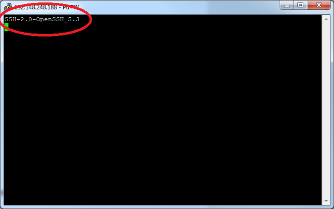
[OSX/Linux] Test your configuration using telnet
- Open a terminal.
- Type
telnet IPaddress 22(Here,IPaddressis IP address listed in "Connections to OSC"). - Confirm the connection.
Connections from OSC
All outbound network traffic from all of OSC's compute nodes are routed through a network address translation host (NAT) including the following IPs:
- 192.148.249.248
- 192.148.249.249
- 192.148.249.250
- 192.148.249.251
IT and Network Administrators
Please use the above information in order to assit users in acessing our resources.
Occasionally new services may be stood up using hosts and ports not described here. If you believe our list needs correcting please let us know at oschelp@osc.edu.
Supercomputer:
Service:
Job and storage charging
Ohio academics should visit the fee structure page for pricing information.
All others should contact OSC Sales for pricing information.
All others should contact OSC Sales for pricing information.
If there are questions/concerns on charging at OSC, please contact OSC Help.
Job charging based on usage
Jobs are charged based length, number of cores, amount of memory, single node versus multi-node, and type of resource.
Length and number of cores
Jobs are recorded in terms of core-hours hours used. Core-hours can be calculated by:
number of cores * length of job
e.g.
A 4 core job that runs for 2 hours would have a total core-hour usage of:
4 cores * 2 hours = 8 core-hours
Amount of Memory
Each processor has a default amount of memory paired along with it, which differs by cluster. When requesting a specifc amount of memory that doesn't correlate with the default pairing, the charging uses an algorithm to determine if the effective cores should be used.
The value for effective cores will be used in place of the actual cores used if and only if it is larger than the explicit number of cores requested.
effective cores = memory / memory per core
e.g.
A job that requests nodes=1:ppn=3 will still be charged for 3 cores of usage.
However, a job that requests nodes=1:ppn=1,mem=12GB, where the default memory allocated per core is 4GB, then the job will be charged for 3 cores worth of usage.
effective cores = 12GB / (4GB/core) = 3 core
Single versus Multi-Node
If requesting a single node, then a job is charged for only the cores/processors requested. However, when requesting multiple nodes the job is charged for each entire node regardless of the number of cores/processors requested.
Type of resource
Depending on the type of node requested, it can change the dollar rate charged per core-hour. There are currently three types of nodes, regular, hugememory,and gpu.
If a gpu node is used, there are two metrics recorded, core-hours and gpu-hours. Each has a different dollar-rate, and these are combined to determine the total charges for usage.
Ohio academics should visit the fee structure page for pricing information.
All others should contact OSC Sales for pricing information.
All others should contact OSC Sales for pricing information.
e.g.
A job requests nodes=1:ppn=8:gpus=2 and runs for 1 hour.
The usage charge would be calculated using:
8 cores * 1 hour = 8 core-hours
and
2 gpus * 1 hour = 2 gpu-hours
and combined for:
8 core-hours + 2 gpu-hours
Project storage charging based on quota
Projects that request extra storage be added are charged for that storage based on the total space reserved (i.e. your quota).
The rates are in TB per month:
storage quota in TB * rate per month
Ohio academics should visit the fee structure page for pricing information.
All others should contact OSC Sales for pricing information.
All others should contact OSC Sales for pricing information.
Please contact OSC Help with questions/concerns.
Out-of-Memory (OOM) or Excessive Memory Usage
Problem description
A common problem on our systems is that a user's job causes a node out of memory or uses more than its allocated memory if the node is shared with other jobs.
If a job exhausts both the physical memory and the swap space on a node, it causes the node to crash. With a parallel job, there may be many nodes that crash. When a node crashes, the OSC staff has to manually reboot and clean up the node. If other jobs were running on the same node, the users have to be notified that their jobs failed.
If your job requests less than a full node, for example, --ntasks-per-node=4, it may be scheduled on a node with other running jobs. In this case, your job is entitled to a memory allocation proportional to the number of cores requested. For example, if a system has 4.5 GB per core and you request one core, it is your responsibility to make sure your job uses no more than 4.5 GB. Otherwise your job will interfere with the execution of other jobs.
Example errors
# OOM in a parallel program launched through srun
slurmstepd: error: Detected 1 oom-kill event(s) in StepId=14604003.0 cgroup. Some of your processes may have been killed by the cgroup out-of-memory handler. srun: error: o0616: task 0: Out Of Memory
# OOM in program run directly by the batch script of a job
slurmstepd: error: Detected 1 oom-kill event(s) in StepId=14604003.batch cgroup. Some of your processes may have been killed by the cgroup out-of-memory handler.
Background
Each node has a fixed amount of physical memory and a fixed amount of disk space designated as swap space. If your program and data don’t fit in physical memory, the virtual memory system writes pages from physical memory to disk as necessary and reads in the pages it needs. This is called swapping.
You can find the amount of usable memory on our system at default memory limits. You can see the memory and swap values for a node by running the Linux command free on the node.
In the world of high-performance computing, swapping is almost always undesirable. If your program does a lot of swapping, it will spend most of its time doing disk I/O and won’t get much computation done. Swapping is not supported at OSC. Please consider the suggestions below.
Suggested solutions
Here are some suggestions for fixing jobs that use too much memory. Feel free to contact OSC Help for assistance with any of these options.
Some of these remedies involve requesting more processors (cores) for your job. As a general rule, we require you to request a number of processors proportional to the amount of memory you require. You need to think in terms of using some fraction of a node rather than treating processors and memory separately. If some of the processors remain idle, that’s not a problem. Memory is just as valuable a resource as processors.
Request whole node or more processors
Jobs requesting less than a whole node are those that request less than the total number of available cores. These jobs can be problematic for two reasons. First, they are entitled to use an amount of memory proportional to the cores requested; if they use more they interfere with other jobs. Second, if they cause a node to crash, it typically affects multiple jobs and multiple users.
If you’re sure about your memory usage, it’s fine to request just the number of processors you need, as long as it’s enough to cover the amount of memory you need. If you’re not sure, play it safe and request all the processors on the node.
Reduce memory usage
Consider whether your job’s memory usage is reasonable in light of the work it’s doing. The code itself typically doesn’t require much memory, so you need to look mostly at the data size.
If you’re developing the code yourself, look for memory leaks. In MATLAB look for large arrays that can be cleared.
An out-of-core algorithm will typically use disk more efficiently than an in-memory algorithm that relies on swapping. Some third-party software gives you a choice of algorithms or allows you to set a limit on the memory the algorithm will use.
Use more nodes for a parallel job
If you have a parallel job you can get more total memory by requesting more nodes. Depending on the characteristics of your code you may also need to run fewer processes per node.
Here’s an example. Suppose your job on Pitzer includes the following lines:
#SBATCH --nodes=2
#SBATCH --ntasks-per-node=48
…
mpiexec mycode
This job has 2 nodes worth of memory available to it (specifically 178GB * 2 nodes of memory). The mpiexec command by default runs one process per core, which in this case is 96 copies of mycode.
If this job uses too much memory you can spread those 96 processes over more nodes. The following lines request 4 nodes, giving you a total of 712 GB of memory (4 nodes *178 GB). The -ppn 24 option on the mpiexec command says to run 24 processes per node instead of 48, for a total of 96 as before.
#SBATCH --nodes=4
#SBATCH --ntasks-per-node=48
…
mpiexec -ppn 24 mycode
Since parallel jobs are always assigned whole nodes, the following lines will also run 24 processes per node on 4 nodes.
#SBATCH --nodes=4
#SBATCH --ntasks-per-node=24
…
mpiexec mycode
Request large-memory nodes
Pitzer has 4 huge memory nodes with ~3 TB of memory and with 80 cores. Owens has 16 huge memory nodes with ~1.5 TB of memory and with 48 cores.
Since there are so few of these nodes, compared to hundreds of standard nodes, jobs requesting them will often have a long wait in the queue. The wait will be worthwhile, though, if these nodes solve your memory problem. See the batch limit pages for Owens and Pitzer to learn how to request huge or large memory nodes.
How to monitor your memory usage
Grafana
If a job is currently running, or you know the timeframe that it was running, then grafana can be used to look at the individual nodes memory usage for jobs. Look for the graph that shows memory usage.
OnDemand
You can also view node status graphically using the OSC OnDemand Portal. Under "Jobs" select "Active Jobs." Click on "Job Status" and scroll down to see memory usage.
XDMoD
To view detailed metrics about jobs after waiting a day after the jobs are completed, you can use the XDMoD tool. It can show the memory usage for jobs over time as well as other metrics. Please see the job view how-to for more information on looking jobs.
sstat
Slurm command sstat can be used to obtain info for running jobs.
sstat --format=AveRSS,JobID -j <job-id> -a
During job
Query the job's cgroup which is what controls the amount of memory a job can use:
# return current memory usage cat /sys/fs/cgroup/memory/slurm/uid_$(id -u)/job_$SLURM_JOB_ID/memory.usage_in_bytes | numfmt --to iec-i # return memory limit cat /sys/fs/cgroup/memory/slurm/uid_$(id -u)/job_$SLURM_JOB_ID/memory.limit_in_bytes | numfmt --to iec-i
Notes
If it appears that your job is close to crashing a node, we may preemptively delete the job.
If your job is interfering with other jobs by using more memory than it should be, we may delete the job.
In extreme cases OSC staff may restrict your ability to submit jobs. If you crash a large number of nodes or continue to submit problematic jobs after we have notified you of the situation, this may be the only way to protect the system and our other users. If this happens, we will restore your privileges as soon as you demonstrate that you have resolved the problem.
For details on retrieving files from unexpectedly terminated jobs see this FAQ.
For assistance
OSC has staff available to help you resolve your memory issues. See our client support request page for contact information.
Service:
XDMoD Tool
XDMoD Overview
XDMoD, which stands for XD Metrics on Demand, is an NSF-funded open source tool that provides a wide range of metrics pertaining to resource utilization and performance of high-performance computing (HPC) resources, and the impact these resources have in terms of scholarship and research.
How to log in
Visit OSC's XDMoD (xdmod.osc.edu) and click 'Sign In' in the upper left corner of the page.
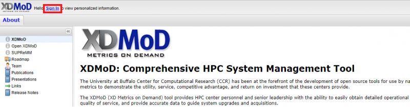
A login window will appear. Click the button 'Login here.' under the 'Sign in with Ohio SuperComputer Center:', as shown below:
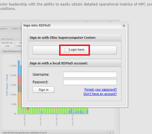
This redirects to a login page where one can use their OSC credentials to sign in.
XDMoD Tabs
When you first log in you will be directed to the Summary tab. The different XDMoD tabs are located near the top of the page. You will be able to change tabs simply by click on the one you would like to view. By default, you will see the data from the previous month, but you can change the start and end date and then click 'refresh' to update the timeframe being reported.

Summary:
The Summary tab is comprised of a duration selector toolbar, a summary information bar, followed by a select set of charts representative of the usage. The Summary tab provides a dashboard that presents summary statistics and selected charts that are useful to the role of the current user. More information can be found at the XDMoD User Manual.
Usage:
The Usage tab is comprised of a chart selection tree on the left, and a chart viewer to the right of the page. The usage tab provides a convenient way to browse all the realms present in XDMoD. More information can be found at the XDMoD User Manual.
Metric Explorer:
The Metric Explorer allows one to create complex plots containing multiple multiple metrics. It has many points and click features that allow the user to easily add, filter, and modify the data and the format in which it is presented. More information can be found at the XDMoD User Manual.
App Kernels:
The Application Kernels tab consists of three sub-tabs, and each has a specific goal in order to make viewing application kernels simple and intuitive. The three sub-tabs consist of the Application Kernels Viewer, Application Kernels Explorer, and the Reports subsidiary tabs. More information can be found at the XDMoD User Manual.
Report Generator:
This tab will allow you to manage reports. The left region provides a listing of any reports you have created. The right region displays any charts you have chosen to make available for building a report. More information can be found at the XDMoD User Manual.
Job Viewer:
The Job Viewer tab displays information about individual HPC jobs and includes a search interface that allows jobs to be selected based on a wide range of filters. This tab also contains the SUPReMM module. More information on the SUPReMM module can be found below in this documentation. More information can be found at the XDMoD User Manual.
About:
This tab will display information about XDMoD.
Different Roles
XDMoD utilizes roles to restrict access to data and elements of the user interface such as tabs. OSC client holds the 'User Role' by default after you log into OSC XDMoD using your OSC credentials. With 'User Role', users are able to view all data available to their personal utilization information. They are also able to view information regarding their allocations, quality of service data via the Application Kernel Explorer, and generate custom reports. We also support the 'Principal Investigator' role, who has access to all data available to a user, as well as detailed information for any users included on their allocations or project.
References, Resources, and Documentation
Job Viewer
The Job Viewer Tab displays information about individual HPC jobs and includes a search interface that allows jobs to be selected based on a wide range of filters:
1. Click on the Job Viewer tab near the top of the page.
2. Click Search in the top left-hand corner of the page

3. If you know the Resource and Job Number, use the quick search lookup form discussed in 4a. If you would like more options, use the advanced search discussed in 4b.
4a. For a quick job lookup, select the resource and enter the job number and click 'Search'.

4b. Within the Advanced Search form, select a timeframe and Add one or more filters. Click to run the search on the server.
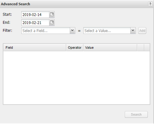
5. Select one or more Jobs. Provide the 'Search Name', and click 'Save Results' at the bottom of this window to view data about the selected jobs.
6. To view data in more details for the selected job, under the Search History, click on the Tree and select a Job.
7. More information can be found in the section of 'Job Viewer' of the XDMoD User Manual.
XDMoD - Checking Job Efficiency
Intro
XDMoD can be used to look at the performance of past jobs. This tutorial will explain how to retreive this job performance data and how to use this data to best utilize OSC resources.
First, log into XDMoD.
See XDMoD Tool webpage for details about XDMoD and how to log in.
You will be sent to the Summary Tab in XDMoD:
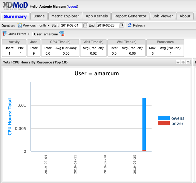
Click on the Metric Explorer tab, then navigate to the Metric Catalog click SUPREMM to show the various metric options, then Click the "Avg CPU %: User: weighted by core hour " metric.
A drop-down menu will appear for grouping the data to viewed. Group by "CPU User Value
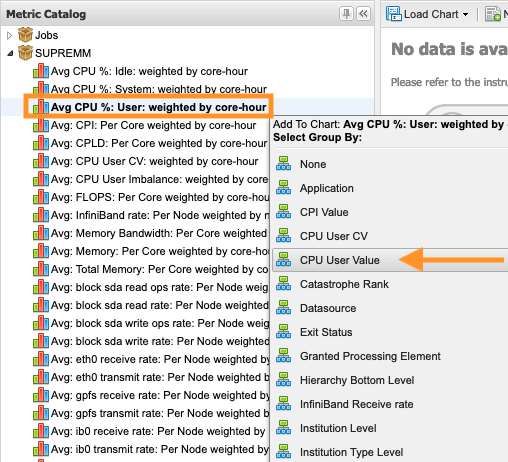 ":
":
This will provide a time-series chart showing the average 'CPU user % weighted by core hours, over all jobs that were executing' separated by groups of 10 for that 'CPU User value'.
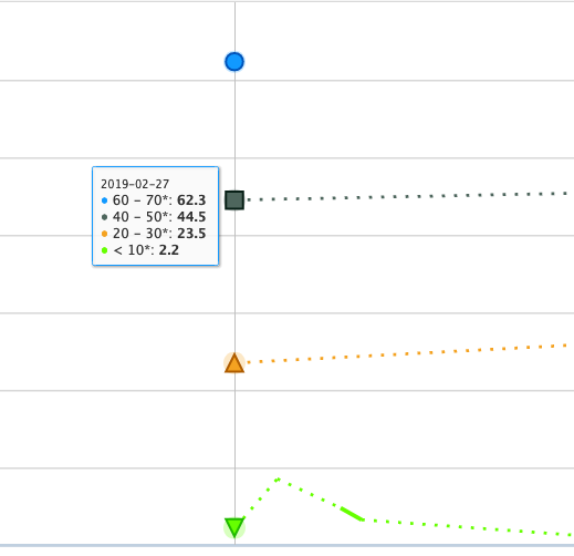
One can change the time period by adjusting the preset duration value or entering dates in the "start" and "end" boxes by selecting the calendar or manually entering dates in the format 'yyyy-mm-dd'. Once the desired time period is entered the "Refresh" button will be highlighted yellow, click the "Refresh" button to reload that time period data into the chart.
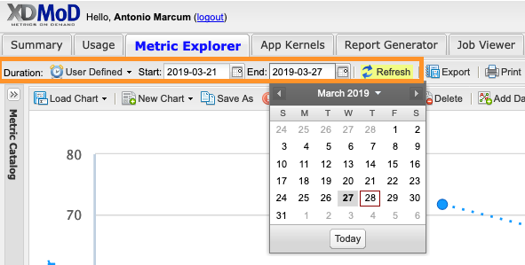
Once the data is loaded, click on one of the data points, then navigate to "Drilldown" and select "Job Wall Time". This will group the job data by the amount of wall time used.
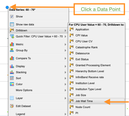
Generally, the lower the CPU User Value, the less efficient that job was. This chart can now be used to go into some detailed information on specific jobs. Click one of the points again and select "Show raw data".
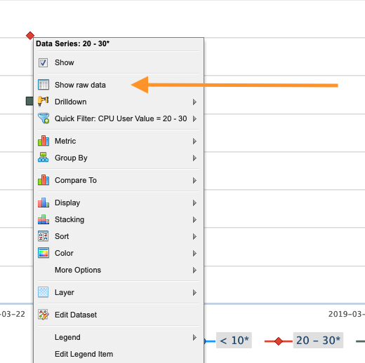
This will bring up a list of jobs included in that data point. Click one of the jobs shown.
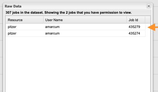
After loading, this brings up the "Job Viewer" Tab for showing the details about the job selected.
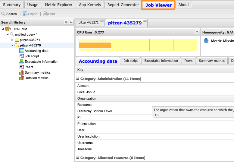
It is important to explain some information about the values immediately visible such as the "CPU User", "CPU User Balance" and "Memory Headroom".
The "CPU User" section gives a ratio for the amount of CPU time used by the job during the time that job was executing, think of it as how much "work" the CPUs were doing doing execution.
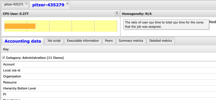
The "CPU User Balance" section gives a measure for how evenly spread the "work" was between all the CPUs that were allocated to this job while it was executing. (Work here means how well was the CPU utilized, and it is preferred that the CPUs be close to fully utilized during job execution.)
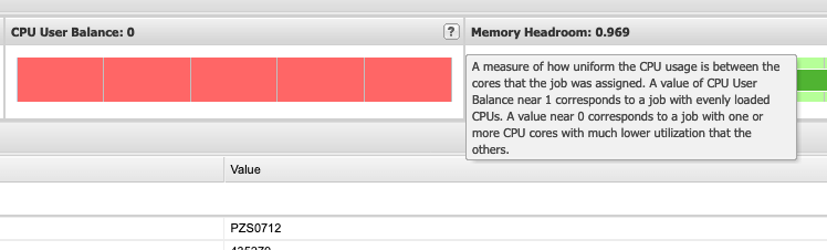
Finally, "Memory Headroom" gives a measure for the amount of memory used for that job. It can be difficult to understand what a good value is here. Generally, it is recommended to not specifically request an amount of memory unless the job requires it. When making those memory requests, it can be beneficial to investigate the amount of memory that is actually used by the job and plan accordingly. Below, a value closer to 0 means a job used most of the memory allocated to it and a value closer to 1 means that the job used less memory than the job was allocated.
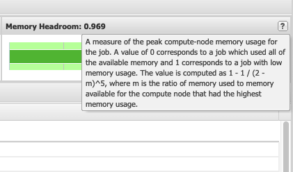
This information is useful for better utilizing OSC resources by having better estimates of the resources that jobs may require.
Gateways
We provide a number of web portals to help our user community easily access and manage computing resources. This guide lists portals of general interest to most OSC clients as well as domain-specific portals. OSC staff also can offer suggestions for more specialized research portals.
General Interest for Most Clients
OSC OnDemand
OSC OnDemand is our "one stop shop" for access to our High Performance Computing resources. With OnDemand, you can upload and download files, create, edit, submit, and monitor jobs, run GUI applications, and connect via SSH, all via a web broswer, with no client software to install and configure.
Access OnDemand | Documentation
Client Portal
The client portal provides access to OSC's accounting and account management infrastructure. Change your password, update contact information, submit budget requests, manage access to research projects, run custom reports, and report funding and publications relevant to your use of OSC services.
Access Client Portal | Documentation
XDMoD
XDMoD, which stands for XD Metrics on Demand, is an NSF-funded open source tool that provides a wide range of metrics pertaining to resource utilization and performance of high-performance computing (HPC) resources, and the impact these resources have in terms of scholarship and research.
Grafana
Query, visualize, alert on and understand your data no matter where it’s stored. With Grafana you can create, explore and share all of your data through a flexible dashboard.
Access Grafana | Documentation
Domain-specific Portals
WebMO
WebMO is a free web-based interface for computational chemistry packages, improving the accessiblity and usability of the software.
Opacity Project
This international collaboration was formed to calculate the extensive atomic data required to estimate stellar envelope opacities and to compute Rosseland mean opacities and other related quantities.
Access Opacity Project | Documentation
phylogatR
Phylogatr brings together genetic data with georeferenced specimen records that are analysis-ready. Analyze the data on the OSC clusters using R scripts or R Shiny apps provided by the phylogatr team.
Access phylogatR | Documentation
Examples of Other Specialized Portals
- BISR (Biomedical Informatics Shared Resource)
- CryoSPARC
- OSUNDA (The Ohio State University resource)
- CATS (Covid-19 Analytics and Targeted Surveillance System)
- Human Genetics Data Management Platform
Please contact OSC Help if you would like to learn more about any of the above.
Client Portal
See Ohio Academic Fee Structure page for more information regarding changes to academic charging.
The url of the OSC client portal is https://my.osc.edu. Please log into it using your current OSC HPC username and password.
Overview
OSC client portal is a full replacement of OSC’s accounting and account management infrastructure (including my.osc.edu and app.osc.edu). It maintains the ability to change your password and contact information as well as submit budget requests, but much is being added. A partial list includes:
- Self-signup for accounts
- PIs or their designates can manage user access to research projects
- Ability to report funding and publications relevant to your use of OSC services
- Ability to run custom reports on usage and annotate jobs
See the navigation sections, one below and one on the right side of the page, for some guides on using the client portal.
Service:
Self-Signup for Accounts
Self-Signup for Accounts
1. Navigate to MyOSC, our client portal.
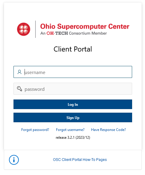
2. Click the "Sign Up" button and submit the form.
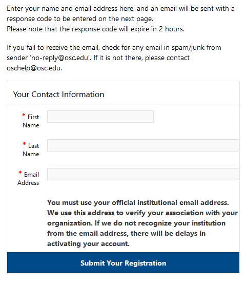
3. Enter the response code.
The response code is only valid for 4 hours. Please contact OSC Help if it is expired.
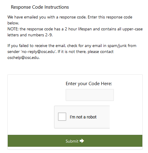
4. The user registration page will be displayed. Please follow the instructions on the page and also fill it out as completely as possible.
If your PI has provided you with a project and/or access code, please enter that information in the correct box. If the project code is provided, you will be added to the project after the PI or Project Admin accepts your request. If both the project code and corresponding access code are provided, you will be added to the project as soon as the sign-up process is complete.
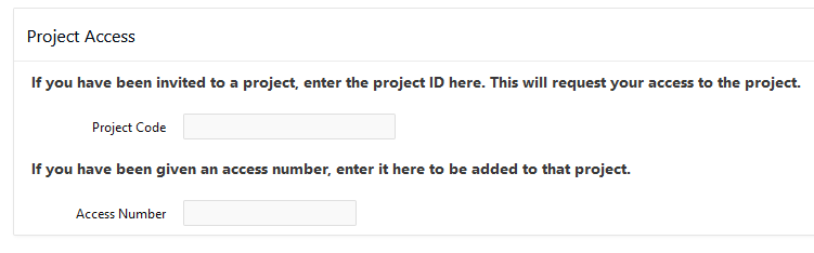
Once all required information is entered, hit the save button to submit the registration.
If you used a non-institutional email address or your institution is not "verified" at OSC, you will see the following:
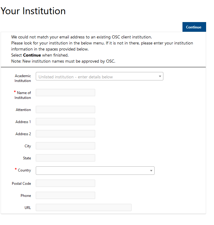
Use the search box to find the appropriate academic institution. If it is not found or you are from a non-academic institution, enter the institution credentials.
5. You now need to accept or decline our terms of use.
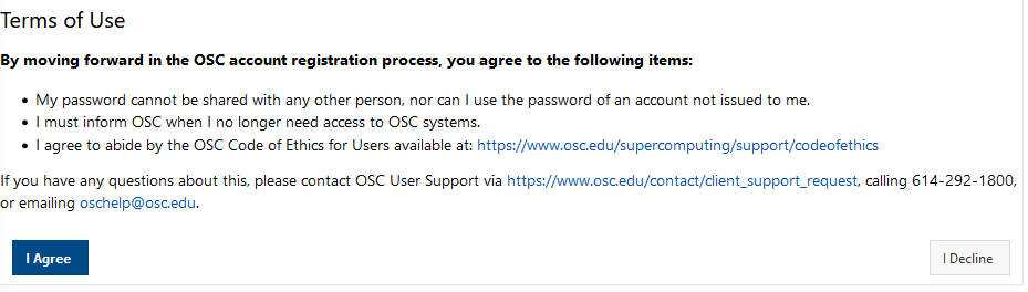
6. If you agree, you can create your username and password. You will not be able to enter the "Confirm Password" section until all of the requirements on the right-hand side are fulfilled (pips will turn green).
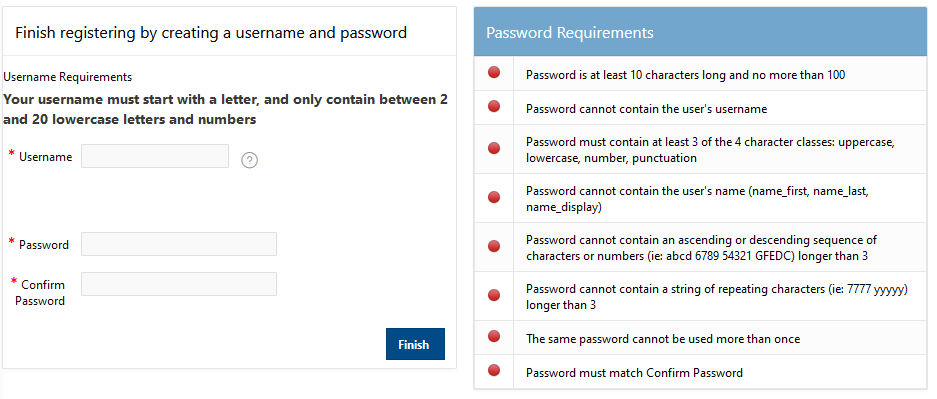
7. Once a username and password are created and saved, there is a redirect back to the login page. The login page will also have a pop-up stating that the username and password have been successfully created.
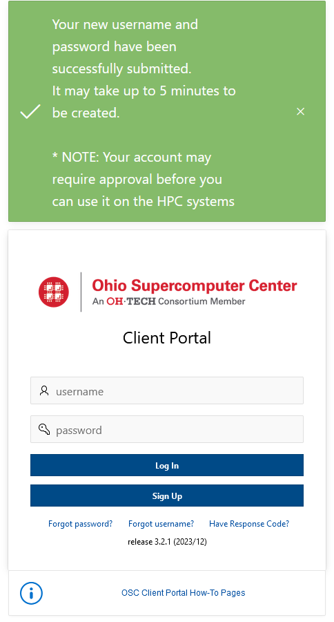
OSC must review and approve any client that is not from an Ohio academic institution. OSC must manually review any client that manually entered their institution. Until this review process, the account will not be able to log into MyOSC or any HPC systems.
Service:
Change or Reset Password and Retrieve Usernames
Client portal password and username options
Please visit MyOSC, our client portal website.
Change password while already logged in
Click "Change Password" from the dropdown menu in the upper-right corner where the full name of the user is shown.
A successful password change redirects back to the dashboard page. There is also a message displayed confirming the change and providing other information.
Reset an expired or forgotten password
From the Login page, click the "Forgot your password?" link.
Enter a valid username and click the "Submit" button. You will be taken to the response code validation page. An email will be sent to the email address associated with that username with the response code to be entered. The email will be sent from "no-reply@osc.edu." All folders should be checked, including spam/junk. If you did not receive this email, please contact OSC Help.
The response code is only valid for 2 hours.
Obtain OSC usernames
To obtain all the usernames associated with an email address, click "Forgot your username?" and enter a valid email address.
This will send an email containing all the associated usernames with the email address entered. The email will be sent from "no-reply@osc.edu." All folders should be checked, including spam/junk. If you did not receive this email, please contact OSC Help.
Service:
Adding grant information
There are different requirements for being able to charge OSC usage towards a grant. This page aims to provide general guidelines, but actual requirements may be different. Contact OSC help if there are specific questions/needs.
Adding grant information
First, the grant information should be added to a user's profile. Login into my.osc.edu and visit the Contact Profile page for the account by clicking the name of the account in the upper-right corner of the page and selecting Edit My Profile.
On this page, click the button Funding, then on the next page click Add New Contact Funding. Enter the appropriate information for the grant and save it.
If a specific funding source is not available, a new one can be created using Individual -> Funding -> Funding Sources, then select Request New Funding Source. This will inform OSC staff to add the new funding source as an option once reviewed.
Use job names
When submitting jobs, make sure to designate the job name to reflect which grant this job applies to.
One can specify the job name at submission time: $ sbatch -J grant_1234 job.sh
Or add a line to the job script: #SBATCH -J grant_1234
This name will be saved with the job record, associating it with the grant specified.
Add a Grant per project
Some grants have strict requirements, and the best way to associate usage for that grant is with a single project, separate from other OSC project's usage. This way, every job associated with a specific project code e.g. PAS1234, will also be implicitly associated with a specific grant.
Visit the project details page for the project that should have grant information added. Click the button External Funding. Select the appropriate grant which should have been added to the PI's profile as in the Adding grant information section above, and click the Add to this project button.
Check usage costs for current fiscal year
It is useful to take a look at usage over periods of time and calculate overall usage at osc. This page explains how to do this using the HPC Job Activity tool in my.osc.edu
After logging into the client portal, navigate to Individual -> HPC Job Activity.
Enter the appropriate dates:
min date: 01 July 2020
max date: current date (or other end date)
Once the dates are entered, the click the button Refresh Report.
It will then produce a table with all the job records within that timeframe.
Group the records together
Select Actions -> Group by
In the drop-down box with text - Select Group by Column - , select Project.
Directly under this, click Add Group by Column and select Charge Type.
Next, use the Sum function with the Dollar Charge column.
Finally, select a format mask and check the sum box on the end of the row.
The format mask can be manually altered to provide more precision.
e.g. FML999G999G999G999G990D0000 will give a dollar amount to the nearest ten-thousandth instead of the deafult hundreth (there are two extra zeroes on the end in the string above).
e.g. FML999G999G999G999G990D0000 will give a dollar amount to the nearest ten-thousandth instead of the deafult hundreth (there are two extra zeroes on the end in the string above).
See the following screenshot to verify the setup:
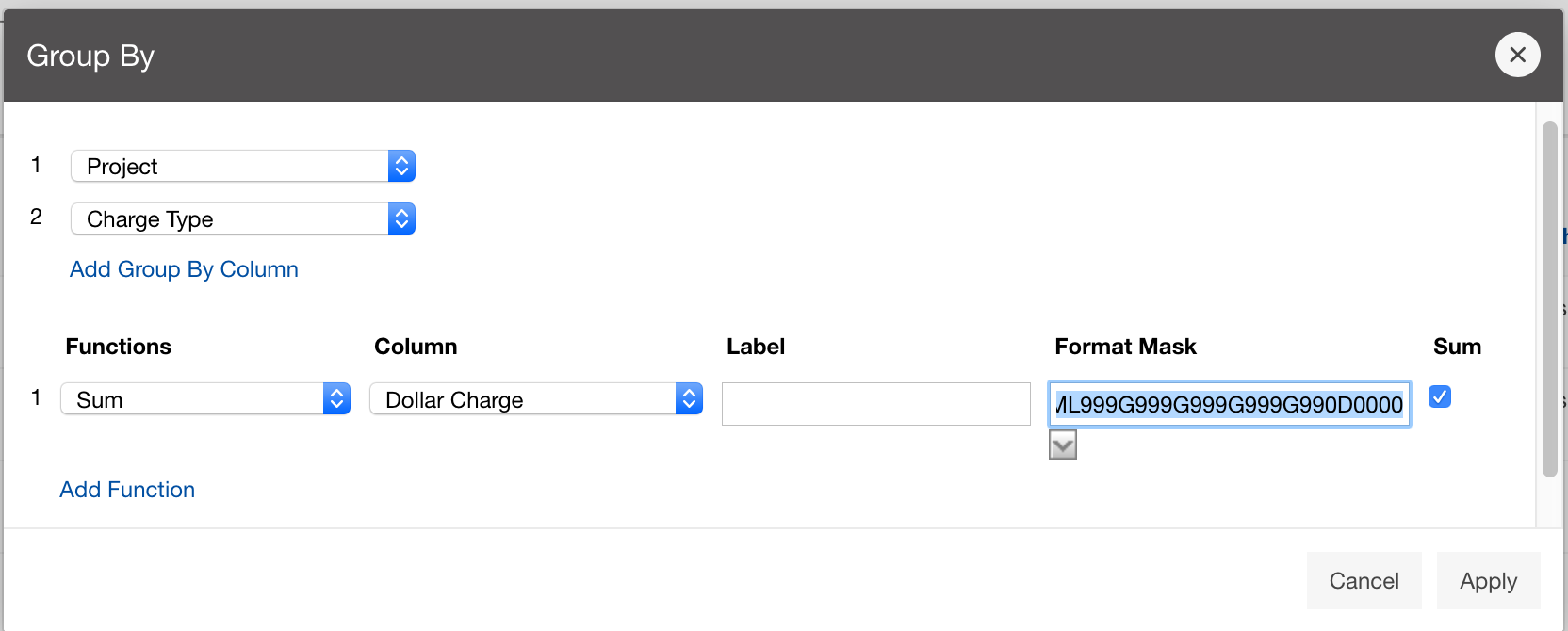
Make sure to save the report just created!
Actions -> Report -> Save Report
Actions -> Report -> Save Report
Export reports
The reports created above can also be saved locally as a csv. Select Actions -> Download and click the available format to download.
Service:
Invite, add, remove users
Manage users on a project
The PI of a project can manage the users on their projects. Note, that PIs are not automatically added as authorized users under their project(s).
Managing users on the project includes inviting, adding and removing users to the project as well as increasing a user's privileges on a project so that they can assist with the management of it.
To manage a project, navigate to Project -> List Projects and select the blue button on the left of the appropriate project.
Adding users
Users can be added to the project by visiting the project details page and selecting the Project Users button. If the user already has an OSC account, then go to Current Project Members -> Add Project User and search them by display name or username. If the user does not have an OSC account, then they can be sent an invitation to sign up for an account and be immediately added to the project by going to Member Invitations -> Invite New User. An email will be sent from "no-reply@osc.edu" - all folders should be checked, including spam/junk. If they did not receive this email, please contact OSC Help.
Approving users
A user may request access to a project, which then needs approved by the PI or a project admin. Navigate to the project details page and select the Project Users button. Expand Current Project Members. Click the blue button next to a username that shows PI approved as no. Set to yes and save. The user should now be approved as a member of the project.
Setup project access number
A user can automatically add themselves to a project if they have the project code and a valid project access number.
The PI or project admin can create a project access number from the project details page using the project access number section and clicking the 'add/replace' button.
The project access number default to be valid only for 14 days. It can be set for less, but 14 is the maximum.
Users may either enter this project access number at sign up or if they already have an account, login and navigate to Project -> Project Access Request. If signing up for an account, an email will be sent from "no-reply@osc.edu" - all folders should be checked, including spam/junk. If they did not receive this email, please contact OSC Help.
Invite users
From your project details, navigate to Current Project Members -> Member Invitations -> Invite New User. Fill in the information and send invite. After complete, the current invitations and project members can be viewed in Member Invitations and Current Project Members respectively.
OSC only allows a single account per person, so users should contact PIs with the email to user or their username to be manually added to the project.
An email will be sent from "no-reply@osc.edu" - all folders should be checked, including spam/junk. If they did not receive this email, please contact OSC Help.
The invitation links are valid for 48 hours. If a link has expired, you will have to complete the form again. If the code has yet to expire, it will show in the show in the table and you can resend.
A complete sign up with result in username appearing in your Current Project Members table.
Removing users
Users can be removed by visiting the project details page and clicking Project Users -> Current Project Members and clicking the blue button left of the username in the list. Select Remove. Many users can be removed more easily by activating the red Enable Quick Removal/Approval button while in the Current Project Members section. There will then be a new column with a  symbol. Click the icon to delete the user instantly.
Invitations can also be deleted by navigating to Member Invitations and selecting the icon on the left of the invite.
Manage user roles
Users can be assigned an admin role on a project by the PI and other project admins. A user can be assigned this role by navigating to the project details page and clicking Project Users -> Administrative Roles -> Add User Role. The only two roles that should be used are Project, Admin Access and Project, No Admin Notifications. Both roles allow a normal user to manage the project as if they were the PI. This allows them to renew the project and manage all users on it.
The PI should designate a Project admin carefully, as they essentially act on the PIs' behalf when managing the project and have FULL privileges.
Service:
Limiting charges with budgets
OSC offers the use of budgets to limit the amount of charges incurred on projects.
Active budget
Once a budget has been approved, it (and the project it was requested from) becomes active. Having an active project allows users on that project to submit batch jobs to use OSC resources.
Using a budget
As usage is accrued on a project, the remaining budget value seen on the project details page will decrease. Once the value of the remaining budget is zero or less, then the project will be restricted and that project can longer be used to submit batch jobs for OSC resources.
Project storage also reduces the remaining budget daily. Project storage is any amount of storage requested by the PI or project admin and is located in either /fs/project or /fs/ess directories.
Home directory locations in /users and scratch locations in /fs/scratch do not count as project storage and are free.
Budgets are a Soft limit
A budget is not going to limit incurred charges to exactly the amount set. Depending on the situation, it could be over by a certain amount. If there are questions/concerns with a budget not correctly limiting charges at OSC, please contact OSC Help.
Once per day operations
The remaing budget amount is not a real-time representation. Completed jobs are uploaded to the client portal once per day. If one looked at their remaining budget and saw $5 was left, but a job that was completed and not yet uploaded to client used $4 worth of resources, then the actual remaining budget should be $1. The same goes for jobs which are still running, except it is unknown how much a running job will reduce the remaining budget by.
Shortly after job records are uploaded to client portal, this adjusts each projects remaining balance based on usage. At this time, if a remaining budget was zero or less, then the project will become restricted and no more jobs can be submitted using that project code.
If a job was already queued or running, before the project became restricted, then this project can still run and use OSC resources. Remember, a restricted project can only stop submission of jobs.
Storage charges
The charges incurred by project storage are not affected by a project becoming restricted.
To stop incurring charges due to project storage, immediately contact OSC Help.
Manage profile information
Edit profile
Profile information can be changed by logging in with valid OSC credentials at MyOSC, navigating to the profile page by clicking the display name in the upper right corner of the page, and selecting Edit my profile.
The page will display information saved for that profile. Some of this information can be freely edited or changed, but other information can only be updated by an OSC admin, such as the institution. Please contact OSC help if there is incorrect information which is not editable.
Email address change
When trying to update an email address, you will need to wait to receive an email and verify the email address change before it will take effect. The email will be sent from "no-reply@osc.edu." All folders should be checked, including spam/junk. If you did not receive this email, please contact OSC Help.
PI status
If you already have an OSC account and want to request PI status to create your own project at OSC, visit the contact profile page.
Look for the Special Access Request section, select the checkbox for "I am an eligible PI" and upload a recent CV document. This will submit a request to OSC staff to review your profile and provide the PI status to your account.
Publications and Funding
There are two buttons for Publications and Funding. The Publications button will bring up a page on which you can manage bibliographic information about publications to reference in account requests or renewals. The Funding button will bring up a page on which you can record funding from other sources to also reference in account requests or renewals.
Only users with a PI status can add information about publications and funding to their profile.
The Publications and Funding pages can also be reached by using the navigation bar and selecting Individual -> Funding or Individual -> Publications.
Information review
Contact information should be verified yearly.
Once a year, after logging into the client portal, you will be redirected to a contact verification page where any out-of-date or incorrect profile information should be updated accordingly.
If there is information that cannot be edited, OSC help should be contacted.
Service:
Multi-factor authentication
MyOSC now supports multi-factor authentication (MFA).
User opt-in
Users can now opt-in to using multi-factor authentication in MyOSC.
On a user's profile page, there will be a button Enable DUO MFA.

There will be an error displayed with the text:
One must log out of MyOSC, then log back in to continue the duo MFA enrollment process where device information can be entered and saved. The next time logging into OSC systems, a duo push will be required to be completed.
Removing MFA
If an OSC account is not required to use MFA, then it can be disabled at any time.
Navigate to your profile page in MyOSC, then select DUO Settings and click the Disable DUO MFA button.
Please note, accessing OnDemand after removing MFA may display an error message that DUO has been disabled. If this happens, please contact OSC Help for assistance.
Project requires MFA
There is also a flag that can be set on a per-project basis, which will require all users on that project to use MFA.
Contact us at OSC Help if you would this enabled on a project.
Supercomputer:
Service:
Project review and special properties
Projects at OSC should be reviewed, at least annually, and OSC staff should be kept up to date on any data with special restrictions being stored at OSC.
Project annual review
Projects at OSC are required to be reviewed annually. This check will be for making sure that only accounts which need to use the project are members of the project, and that all users with admin roles still need that role. Furthermore, it is for checking that the project has an appropriate special property for the data being stored.
You will be prompted upon log in at MyOSC to verify. This will occur 365 days after your last project verification.
If you'd like to verify early, you can do so from the Project Details > Project Users. Now you are on the Manage Project Users table and there is a button to "Verify Project Members and Admins."
OSC has temporarily disabled the ability for PIs to add/remove a special property to projects themselves.
Please contact OSC Help if a special property needs added/removed to a project.
Please contact OSC Help if a special property needs added/removed to a project.
Projects with special data
If a project is storing data that has special restrictions on whom can access that data, then OSC staff should be made aware of this.
The project may be categorized as a protected data project, or the special restrictions could be simpler and just require permissions to be kept reasonably secure (e.g. NIH genomic data policy).
In both cases, the project should be labeled with a special property to explicitly show that data with special restrictions are being stored.
OSC has temporarily disabled the ability for PIs to add/remove a special property to projects themselves.
Please contact OSC Help if a special property needs added/removed to a project.
Please contact OSC Help if a special property needs added/removed to a project.
Projects, budgets and charge accounts
There are significant changes as to how resources are requested within the client portal. More information on the changes can be found at:
Client Portal, MyOSC, documentation
"Ohio Academic Fee Model FAQ" section on our service costs webpage
Client Portal, MyOSC, documentation
"Ohio Academic Fee Model FAQ" section on our service costs webpage
OSC client portal allows users to manage their projects.
Creating a new project
If you already have a project with OSC and want to re-use that project code, please proceed to the budget section of this documentation.
Any user with the Primary Investigator (PI) role can request a new project in the client portal. Using the navigation bar, select Project, Create a new project. Fill in the required information. See more details on these options below.
The pricing implications for requesting a new project should be understood before continuing.
Once the project is created, you need to add authorized users, including yourself, to access the project, i.e. HPC resources.
Project types
Depending on the project type selected here, it will alter how budgets are approved.
The project types academic, commercial, and government/non-profit projects will use the approval process set up by the institution of the PI requesting the project. This could involve waiting on a fiscal approver to review the request, or having the request automatically approved.
The classroom project type will be routed to OSC staff for approval since all usage under a classroom project is fully discounted so that no charges are incurred by the PI. Remember that a syllabus is required for classroom projects to be approved.
Charge accounts
A PI can choose to create a new charge account or select an existing one when creating a new project. The PI will not be able to select anyone else as the owner. If a different owner is needed, please contact OSC Help. Note, the owner of the charge account can request changes to the project(s) under the charge account, including closure.
See "Charge accounts overview" section near the bottom of this page for more information on creating a new charge account.
Use the drop-down box to select an existing charge account. If there is a credit already added to an existing charge account, then the text '(credit: <dollar-amount>)' will show next to the charge account name.
For PI associated with Ohio academic institutions, the annual Ohio academic credit of $1,000 will be added automatically to the charge account selected here, if the credit has not already been added. The credit will be added after the first budget of the fiscal year is approved.
The charge account is important because it is used for credits (such as the annual credit available to Ohio Academics). Many projects can be grouped under a single charge account, which also means many projects can take advantage of that charge account's credits as well.
The $1,000 annual billing credit for Ohio academic PIs is allocated once on a fiscal year basis.
Special properties
Special properties can currently only be added by OSC staff.
If the project will contain sensitive data such as PHI (HIPAA related), ITAR, etc, then contact OSC to use the protected data service which provides controls to keep data secure.
Misc fields
- Project title
- Field of science
Creating a budget
After entering the required information on the project creation page, a budget can be created.
For projects that are already created, head to the project details page and click the Create new budget button, and go through the budget creation process again.
Budgets are used to constrain spending in a fiscal year, but bills are based on service type and utilization. Budgets can be replaced at any time.
Timeframe
First, select the timeframe that the budget should be created for.
The timeframe can either be for this fiscal year or the next fiscal year.
A fiscal year is from July 1st to June 30th the next calendar year.
Budget type
There are two types of available budgets, limited and unlimited.
Limited budgets are used for projects that want to put a maximum on the charges that can be incurred. This is useful for a PI that creates a new project, receives the $1,000 annual credit, then sets a limited budget of $1,000.
Unlimited budgets are for projects that will not have a spending limit.
To create a limited budget, answer yes to 'Do you want to set a dollar budget?'. For an unlimited budget, select no.
If you have a restricted project you want to re-use, you would submit the budget request under that project code.
Org Fiscal Reference text field and checkbox
There are two fields that may need to be filled in.
The Org Fiscal Reference is an internal accounting field for the project's organization.
For e.g. At Ohio State University, a PI should enter the Purchase Request # here.
The Fiscal Approval checkbox is an option displayed for a PI that can automatically activate a budget without requiring review. It has the PI declare that they have already been approved for spending at OSC.
Submit budget review or activating budget
After filling in budget information, the next page will be different depending on whether the PI's institution has set up a review process at OSC.
If the institution allows PIs to activate their own budget, the PI simply clicks Activate Budget, then the project and budget are both set to active.
If the institution requires a review of the budget, an email will be sent to reviewers. Once the reviewers decide on approving, partially approving (an amount different than the PI's request), or rejecting, the PI will receive a notification of the response.
Storage request
Storage can be requested from the project details page. Look for the button request storage change.
The difference between different storage at OSC is described in available file systems.
Storage does have a cost associated with it per TB requested. Once the storage space is created it is considered permanent and it will continue to accrue charges, even if the budget has been depleted and the project is restricted.
Please contact oschelp@osc.edu to request that project storage be removed and no longer charged for.
Please contact oschelp@osc.edu to request that project storage be removed and no longer charged for.
Managing projects
Projects that have been created should be managed periodically.
View all projects
To view all projects, even those not submitted for approval and still waiting on approval, navigate to Project, Project List.
View Budgets
Go to the project details page and select the Budgets button to view current and past budgets.
Charge accounts overview
Create a new charge account
PI's can create a charge account, which allows them to group projects together under that charge account.
To create a new charge account, select from navigation bar Charge account, then Create new charge account or select Project, then create new project and leave charge account selection at Generate a new charge account.
See information on the fields below.
Parent charge account
Every charge account created by a PI must have a parent. Either enter the name of the parent if it is known, or clear the parent charge account selection, then click the button View hierarchy, then Collapse all, to show the available parent charge account options.
With the hierarchy view shown, look for the correct parent charge account. For most academic PI's, there may be a "<institution> top-level" charge account that can be selected. There may also be colleges and department charge accounts under the colleges. Select the correct charge account based on your current position.
In the hierarchy view, only charge accounts showing "PI_AVAILABLE" can be selected as a parent. This can be seen as a suffix to the charge account name listed.
Contact
Leave the contact as your own user account.
Display name
The title of the charge account being created. Can be useful to provide a summary name for the types of projects that will be created under the charge account.
e.g. Creating a charge account to group projects which all use the same funding, or to group projects where the results are all related.
Submit or save for later
Click the submit button to create the new charge account or save for later button to come back to the charge account later.
View credits
Credits can be viewed at Charge account, then Charge account list.
This will display all charge accounts created by you, and a column for "Total dollars given", which is the total credit available for that charge account.
Questions on what is a budget? What is the credit?
Please see service terms for further explanations or contact oschelp@osc.edu
Service:
billing statements
MyOSC now offers the ability for PIs to view the billing statements of current un-billed usage for their projects.
Login to my.osc.edu and navigate to Project -> Billing Statements.
There are two sections:
Current usage
The current usage section provides information usage charges up to the current day.
These are not final charges, as they may be countered by credits or discounts at the time billing is ran.
Statements
The statement section lets PIs view past statements that will include information about charges including discounts and credits applied for that period.
Supercomputer:
Service:
HPC Job Activity tool
Interactive reporting of HPC job activity
The HPC Job Activity menu item opens a powerful reporting tool. By default, the report shows all activity over the last 30 days for projects you are authorized to view usage of. There are simple filters available at the top to put in a specific job ID, narrow the report to a specific project, or select a specific date range.
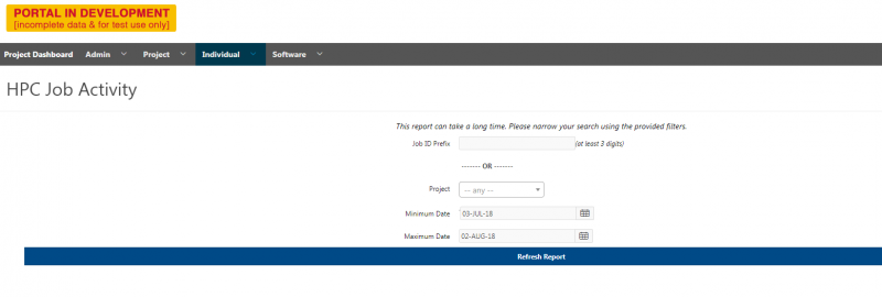
Click ‘Refresh Report’ to get the job activity report as shown below:
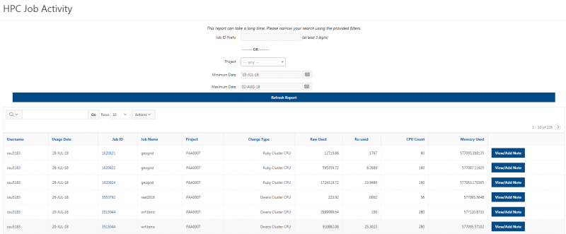
There are more details on how to do advanced reports discussed in ‘Interactive Reporting’ section, but here are some basics about interacting with the report. Clicking on a column header will bring up a quick filter menu where you can filter the records, sort by that column, hide the column, or group by each unique entry.
In addition, you can do a quick text search, select which saved report you wish to view (if you have any saved reports), change the number of rows per page, and do advanced actions from changing the visible columns to aggregating data, creating charts, and saving your custom report formats.
View job scripts
To view the script associated with a job, you can click on the ‘Job ID’ for that job. This will open a pop-up dialog with the first 5kb of the job script, with a button to enable you to download the entire script.
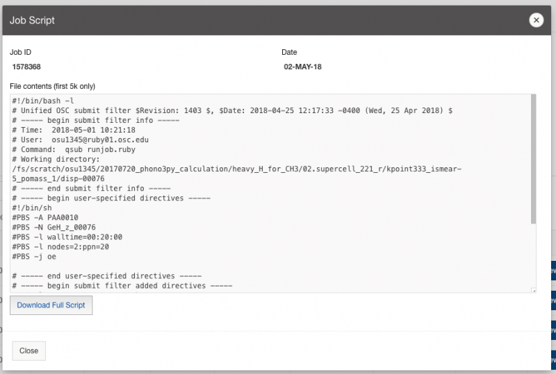
Importantly, you will notice that the script is not identical to what you submitted on the command line; this is because our infrastructure scripts will add some additional information of value to the scheduler and record that information in the final job script.
If a job is interactive, the job script will not be recorded because there isn’t one! We do not have a mechanism to record what happens in an interactive batch job and store that in the accounting system. You may want to use descriptive job names in your batch submissions if you want to be able to review utilization and determine what a job was for when no script is recorded.
Creating a job note
There is a column available in the report that provides a per-row button labeled “View/Add Note”. This button will open a dialog window that will allow you to view any notes that have been added to a job or create a note. At 200 characters, notes are fairly short, but they do allow you to add a little bit of metadata to a job once it is in the accounting system.
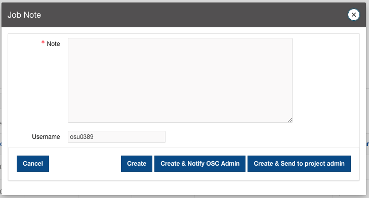
There are three “create” buttons available, which take slightly different actions. Clicking “Create” will just save the note in the job record. Clicking “Create & Notify OSC Admin” will allow you to save the note and notify OSC staff that there is a job note they should review. Please note, this is not the recommended or preferred method for reporting job problems. Please continue to email OSC Help. Finally, “Create & Send to project admin” will add the note to the job record and notify the PI and project admins that there is a job note that needs to be reviewed.
Service:
Interactive Reporting
In the client portal, interactive reporting is provided using Oracle Application Express (APEX) which allows end users to query data and customize reports. This interactive reporting allows users to:
- Customize the layout of the data by choosing the columns they are interested in, applying filters, highlighting, and sorting
- Define breaks, aggregations, different charts, and their own computations
- Create multiple variations of the report and save them as named reports, output to comma-delimited files, and print them to PDF documents
The discussions here are also applicable to other pages where data can be manipulated similarly.
The HPC Job Activity page
Navigate to Individual -> HPC Job Activity.
Click Refresh Report to get the job activity report as shown below. By default, the report shows a table of all activity over the last 30 days for projects you are authorized to view usage of, with 10 rows per page.
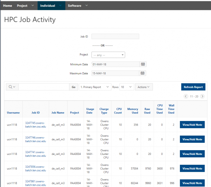
There are simple filters available at the top to put in a specific job ID, narrow the report to a specific project, or select a specific date range. Click “Refresh Report” to update the table with new filters.
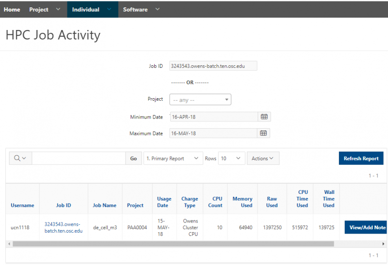
For more advanced functions of using filter, see the discussion of ‘Filter’.
Column sorting and filtering
Many actions can be performed by clicking on a column heading. These include:
- Sorting data (both ascending and descending)
- Hiding the column
- Creating a control break
- Viewing of the column text and the ability to select a value to create a quick filter
Let’s use the column ‘CPU Time Used’ as an example for detailed discussions. Click ‘CPU Time Used’:
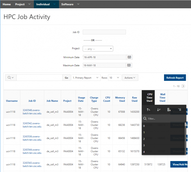
- Click ‘
 ’, and the jobs will be listed based on the value of CPU time in ascending order
 - Click ‘
 ’, and the jobs will be listed based on the value of CPU time in descending order
 - Click ‘
 ’, and the column ‘CPU Time Used’ will be removed from the table
 - Click ‘
 ’, and the table will be split into multiple groups, where each group shares the same value of CPU time
It also lists all the available values of CPU time. You can select a value to create a quick filter, and the table will be updated to list the jobs of which the CPU time is the specified value:
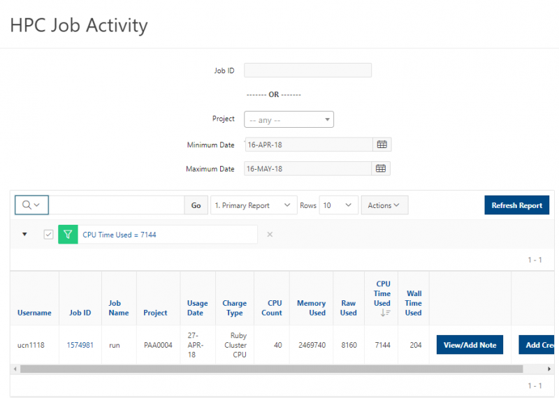
You can also use ‘search’ to narrow down the information to be viewed.
Adjust the displayed information in the table
You can adjust the columns to be displayed in this table to see more/less information. Click ‘Columns’ within the ‘Actions' dropdown menu:
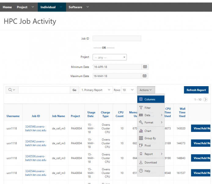
You will get the pop-up window shown below. The columns on the right are displayed. The columns on the left are hidden. Select the information to be displayed using ‘>’; select the information to be NOT displayed using ‘<’. You can also reorder the displayed columns using ‘↑’ and ‘↓’. Click ‘Apply’ button to apply the changes.
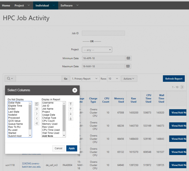
Most columns are self-explanatory. Computed columns are prefixed with **. Definitions of some columns are provided below:
- Project: which project this job is charged to
- Usage Date: the date when this job is charged
- Memory Used: in bytes
- CPU Time Used: in seconds
- Wall Time Used: in seconds
'Search' tool
The ‘Search’ tool enables you to narrow down the displayed report that contains specific text only. To search all columns, simply type the text in the search box and click on ‘Go’ or press ‘Enter’.
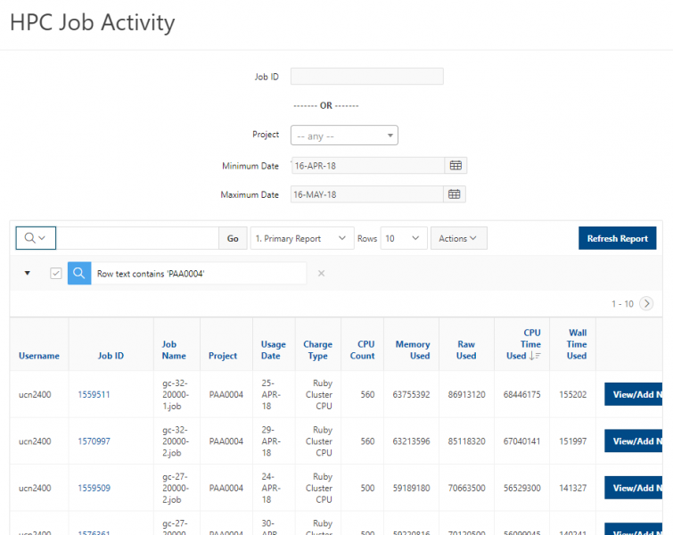
The page will be refreshed automatically to display the results following the search criterion, with the search criterion being listed above the table:

To apply multiple search criteria, add another search criterion after one search criterion is applied. Always remember to hit ‘Enter’ to apply the search criterion:
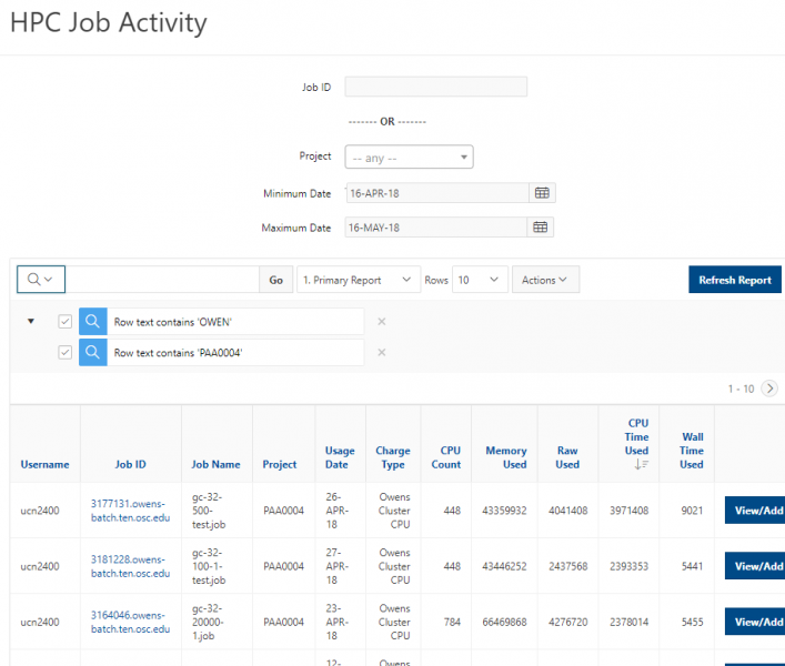
Check the box on the left to display/not display the results following this search criterion. The displayed results will be refreshed automatically:
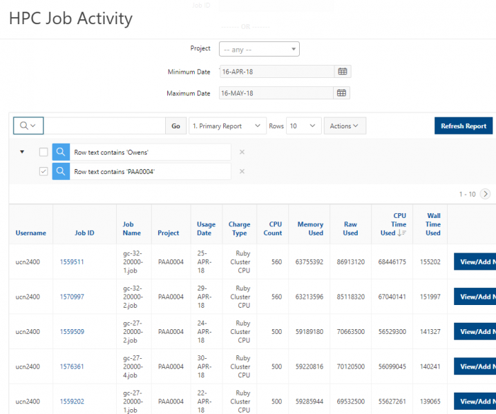
Click the ‘x’ on the right to remove this search criterion. The displayed results will be refreshed automatically:
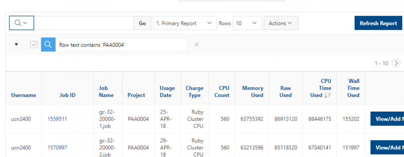
To search one specific column, select the column from the dropdown ‘˅’ to the left of the search box before providing the text in the box:
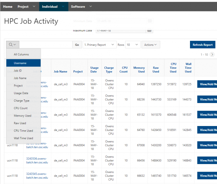
For instance, if you would like to get a report of HPC jobs submitted by user ‘ucn1118’ only, select ‘Username’ from ‘˅’. ‘Search: Username’ will be displayed in the ‘search’ box:
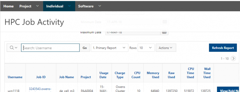
Type ‘ucn1118’ and hit ‘Enter’ in the box, jobs submitted by ‘ucn1118’ only will be displayed in the table, as shown below:
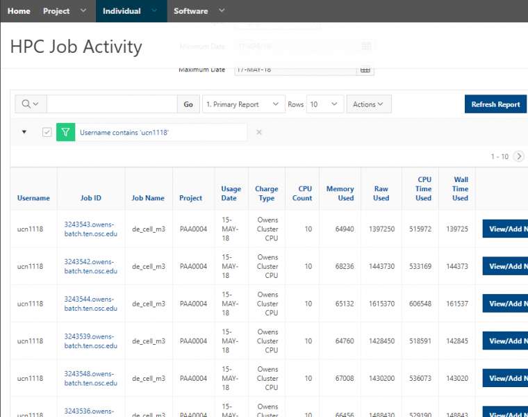
'Actions' menu
The ‘Actions’ menu contains many tasks that are useful in querying data and customizing reports. Click ‘˅’ to get a list of available functions.
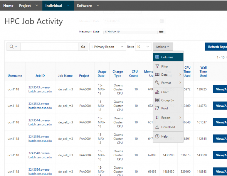
For more information, see: [1] and [2]
Adjust the displayed information in the table
Click ‘Columns’ within the ‘Actions' dropdown menu, you can adjust the columns to be displayed in this table to see more/less information.
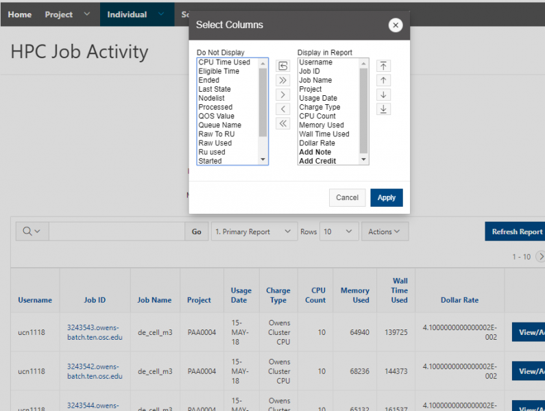
See here for more info: ‘Adjust the displayed information in the table’.
Query data and format report
Within the ‘Actions' dropdown menu, it provides the following tools to query data and format report:
- Filter
- Data
- Format
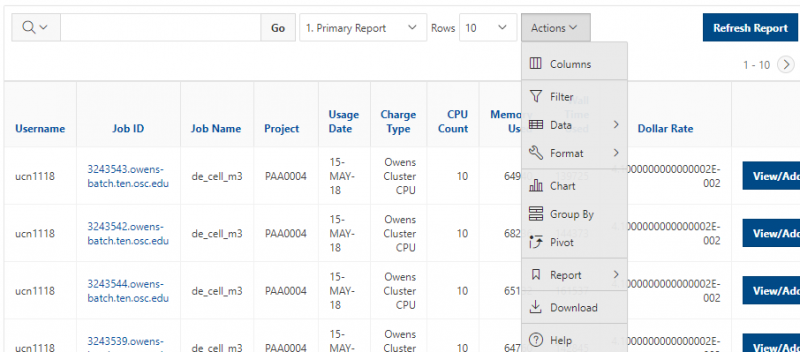
Filter
Click ‘Filter’ within the ‘Actions' dropdown menu as below:
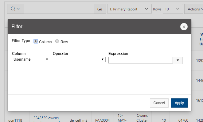
You can create the filter based on either ‘Column’ or ‘Row’.
If you filter by column, select a column using ‘▼’, a standard Oracle operator using ‘▼’, and enter an expression to compare against. Expressions are case sensitive. Use % as a wild card, if needed. You can also select the expression using ‘▼’.
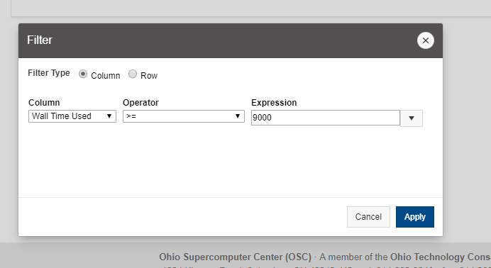
If you filter by ‘Row’, you can create complex WHERE clauses using column aliases and any Oracle functions or operators. Click ‘Apply’ to apply the filter:
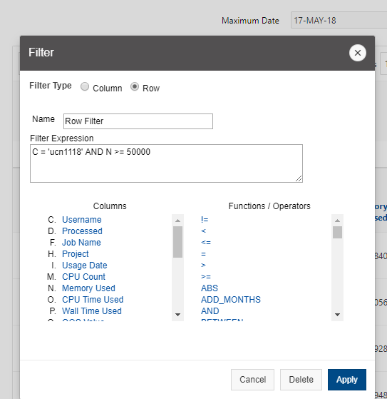
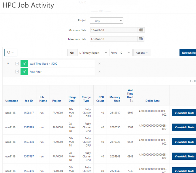
Data
Click ‘Data’ within the ‘Actions' dropdown menu. You can sort data, perform mathematical computation on column, add computed column to your report, and perform a flashback query within ‘Data’ menu.
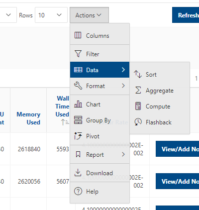
- Sort
It is used to change the columns to sort on and determines whether to sort in ascending or descending order. You can also specify how to handle NULLs. The resulting sorting displays to the right of column headings in the report.
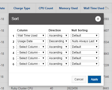
- Aggregate
Aggregates are mathematical computations performed against one column. Click ‘Aggregate’ to get the pop-up window shown below:
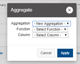
Here, ‘Aggregation’ enables you to select a previously defined aggregation to edit; ‘Function’ is the function to be performed (for example, SUM, MIN); ‘Column’ is used to select the column to apply the mathematical function to. Only numeric columns display.
Click the ‘Apply’ button, the aggregates will be displayed at the end of the report within the column they are defined.
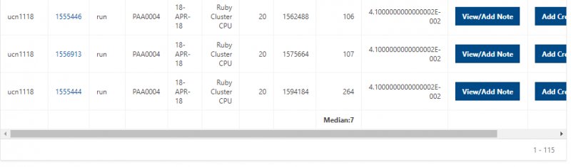
- Compute
It enables you to add computed columns to your report. These can be mathematical computations or standard Oracle functions applied to existing columns. Click ‘Compute’ to get the pop-up window shown below:
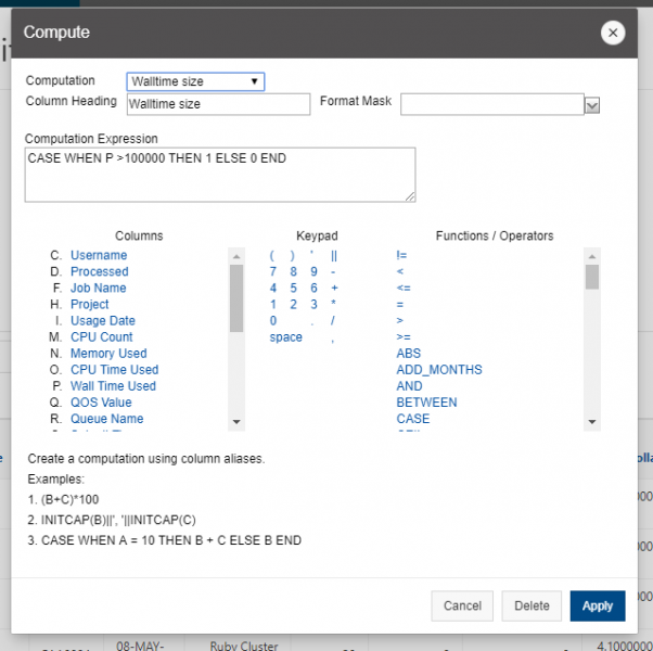
Here, ‘Computation’ enables you to select a previously defined computation to edit; ‘Column Heading’ is the name of this new column displayed in the table; ‘Format Mask’ is an Oracle format mask to be applied against the column; ‘Computation Expression’ is the computation to be performed where columns are referenced using their associated alias. Clicking on the column name or alias includes them in the Computation. Next to Columns is a keypad. This keypad functions as a shortcut to commonly used keys and inserts those keys in the Computation. On the far right are Functions.
Once the computation is defined, click ‘Apply’ button. The computed column will be displayed as the last column of the table.
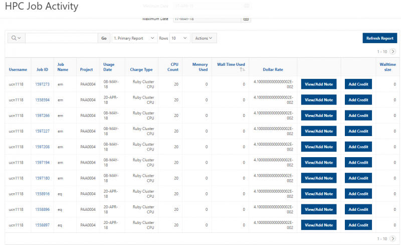
- Flashback
A flashback query enables you to view the data as it existed at a previous point in time. The maximum amount of time that you can flashback is 7047 minutes.
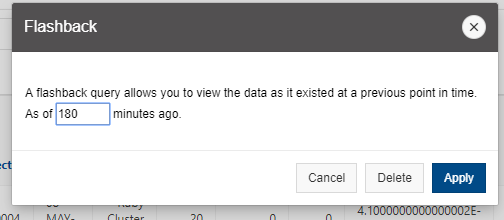
Format
Click ‘Format’ within the ‘Actions' dropdown menu:
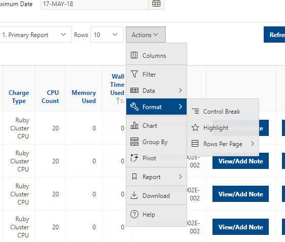
Using ‘Format’ menu, you can split the report into multiple groups, highlight the rows that meet the filter, and modify the number of rows listed per page.
- Control Break
It is used to create a break group on one or several columns. Click ‘Control Break’ to get the pop-up window shown below:
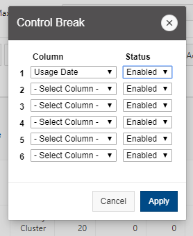
Enable or disable the column for control break. Click ‘Apply’ button. This pulls the columns out of the Interactive Report and displays them as a master record.
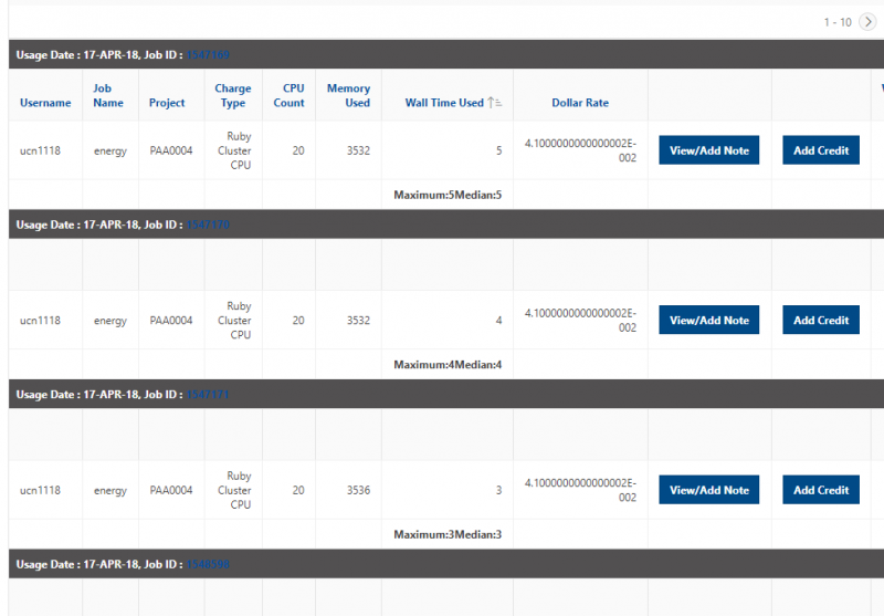
- Highlight
It allows you to define a filter. The rows that meet the filter are highlighted using the characteristics associated with the filter. You can highlight the entire row or just the affected cell and can select a new color both for the background and the text. Click ‘Highlight’ to get the pop-up window as below:
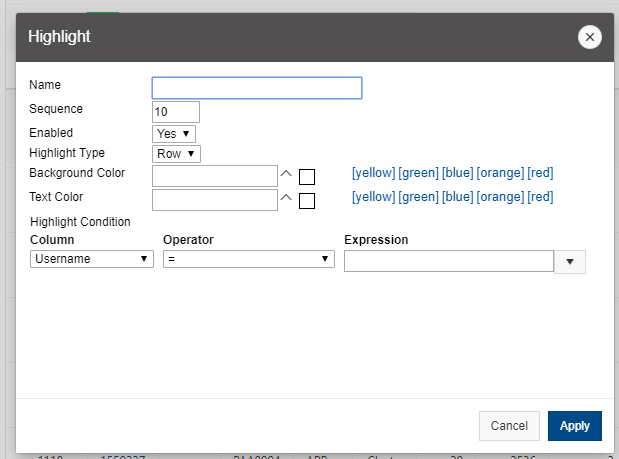
Here, the options include:
- Name: provide a name for this ‘highlight’. Once it is defined, it will be displayed on the top of the table with returned results
- Sequence: identifies the sequence in which the rules are evaluated.
- Enabled: identifies if a rule is enabled or disabled.
- Highlight Type: identifies whether the row or cell should be highlighted. If Cell is selected, the column referenced in the Highlight Condition is highlighted.
- Background Color: is the new color for the background of the highlighted area.
- Text Color: is the new color for the text in the highlighted area.
- Highlight Condition defines the filter condition.
Click the ‘Apply’ button. This pulls the columns out of the Interactive Report and displays the results with defined highlights.
- Rows Per Page
You can select the value to modify the number of rows listed per page.
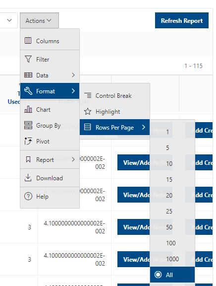
Data visualization
Different tools are available in client portal for the data visualization, including:
- Chart
- Group By
- Pivot
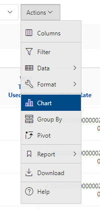
Chart
Click ‘Chart’ to get the pop-up window as below:
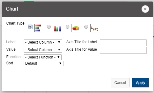
Here, the options include:
- Chart Type: identifies the chart type to include. Select from horizontal bar, vertical bar, pie, or line.
- Label: enables you to select the column to be used as the label.
- Axis Title for Label: is the title that displays on the axis associated with the column selected for Label. This is not available for pie chart.
- Value: enables you to select the column to be used as the value. If your function is a COUNT, a Value does not need to be selected.
- Axis Title for Value: is the title that displays on the axis associated with the column selected for Value. This is not available for pie chart.
- Function: is an optional function to be performed on the column selected for Value.
- Sort: allows you to sort your result set.
Click the ‘Apply’ button. You will get the page in which the chart is generated. You can include one chart per Interactive Report. Once defined, you can switch between the chart and report views using the icons beside ‘Go’:
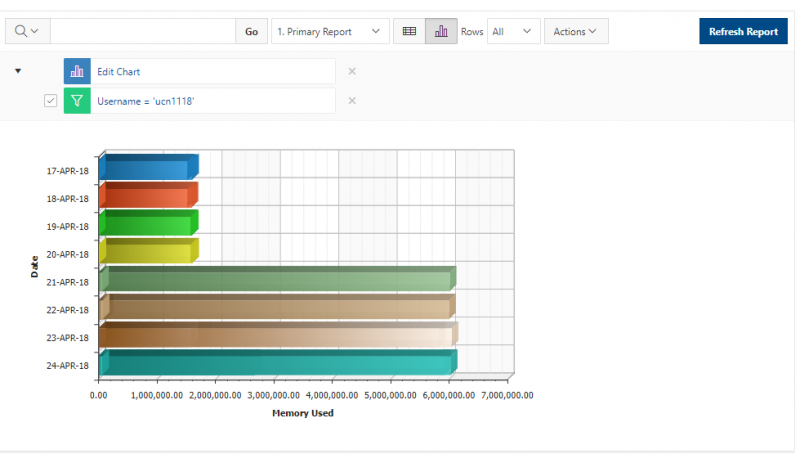
Group By
Click ‘Group By’ to get the pop-up window as below:
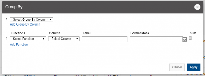
Here, the options include:
- Add Group By Column: the columns on which to group
- Add Function: the columns to aggregate along with the function to be performed
Click the ‘Apply’ button. You will get the page in which the Group By view is generated. You can include one Group By view per Interactive Report. Once defined, you can switch between the Group By and report views using the icons beside ‘Go’:

Pivot
Click ‘Pivot’ to get the pop-up window as below:
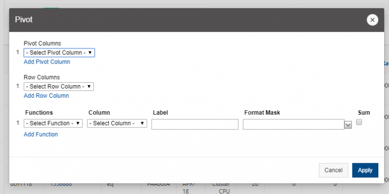
Here, the options include:
- Add Pivot Column: the columns on which to pivot
- Add Row Column: the columns to display as rows
- Add Function: the columns to aggregate along with the function to be performed
Click the ‘Apply’ button. You will get the page in which the Pivot view is generated. Please note that Pivot does not work for very large datasets e.g. ~5000 entries. You can include one Pivot view per Interactive Report. Once defined, you can switch between the Pivot and report views using the icons beside ‘Go’:
Save/Reset report
Within ‘Report’ menu, you can save the customized report for future use, or remove any customizations that you have made and reset the report to the default settings.
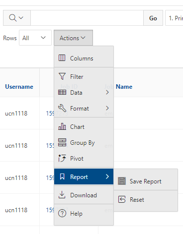
Save Report
‘Save Report’ saves the customized report for future use (it will be there after logging out and back in again). Click Save Report’ to get the pop-up window shown below:
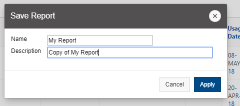
You provide a name and an optional description. For now, all customized reports are private, which means only the end user that created the report can view, save, rename or delete the report. If you save customized reports, a Reports selector displays in the Search bar:

You will be able to choose the reports between ‘Default -> Primary Report’ (which is the report that initially displays) and ‘Private -> Your defined reports’
Reset
‘Reset’ brings the report back to the settings when logged in, removing any customizations that you have made. Click ‘Reset’ to get the pop-up window as below:
Click the ‘Apply’ to confirm. You can also uncheck the checkbox next to any customization to temporarily disable it or click the ‘x’ icon to remove the customization.
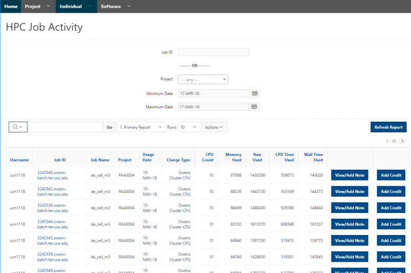
Download
‘Download’ enables the current result set to be downloaded. Click ‘Download’ to get the pop-up window:
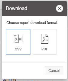
The download formats differ depending upon your installation and report definition but may include CSV, HTML, PDF, or Email. Click the icon of the format you wish to download in.
Help
‘Help’ provides you more detailed user guide on ‘Action’ menu.
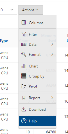
Example: create a chart report of daily HPC jobs by a user
In this example, I’d like to provide step-by-step instructions for creating a chart report of HPC jobs, in which:
- All jobs submitted by user ‘xwang’
- The data range is from April 29, 2018 to May 7, 2018
- The report shows the total CPU time per day
The following functions will be demonstrated:
- Use simple filter on ‘HPC Job Activity’ page
- Use ‘search’ tool
- Adjust rows to be displayed per page
- Adjust columns to be displayed in the table
- Format the data using ‘Control Break’
- Generate a chart report
- Save report
- Download report
- Click ‘Individual -> HPC Job Activity’
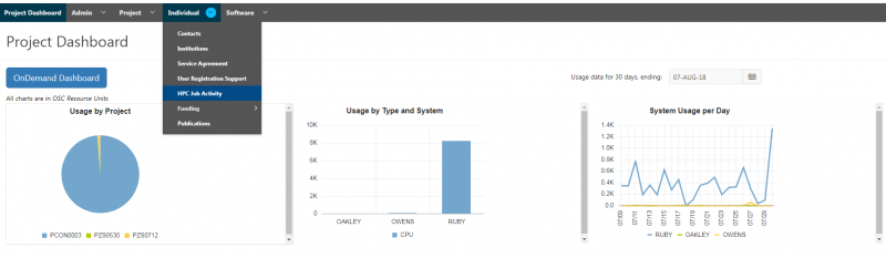
- You will get the ‘HPC Job Activity’ page. Change ‘Minimum Date’ and ‘Maximum Date’ to ‘29-Apr-18’ and ’07-May-18’, respectively. Click “Refresh Report’ to updated the information displayed in the table
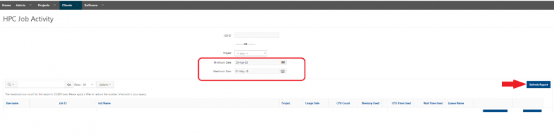
- To listed the jobs submitted by user ‘xwang’ only, click ‘Search’ box and choose ‘Username’:
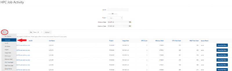
- Type ‘xwang’ in the ‘search’ box and press ‘Enter’.
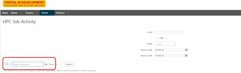
- You will get the table that lists all jobs submitted by user ‘xwang’ between April 29, 2018 and May 7, 2018, with the filter listed above the table. Change the number of rows displayed per page to ‘All’ to list all jobs, as shown below:
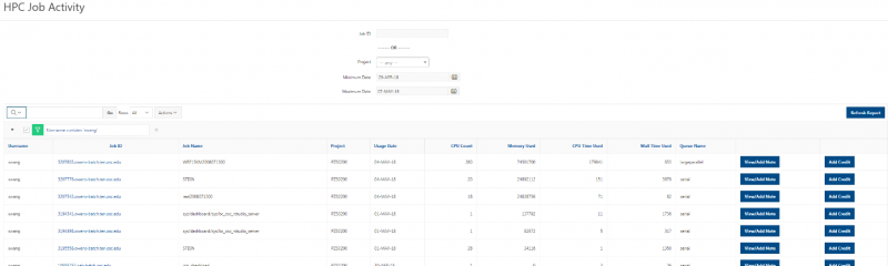
- Since we are interested in the daily CPU usage by ‘xwang’, we can remove some columns of the table by clicking the heading of some columns to hide the column. For instance, click ‘Hide Column’ icon in ‘Job ID’, the page will be refreshed automatically. The column ‘Job ID’ will NOT be displayed after refreshing:
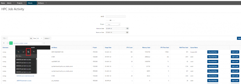
- Perform similar operations on other columns. You can also adjust the columns to be displayed by clicking ‘Columns’ within the ‘Actions' dropdown and make ‘Username’, ‘Usage Date’, and ‘CPU Time Used’ to be displayed in the report. The final table is as below:
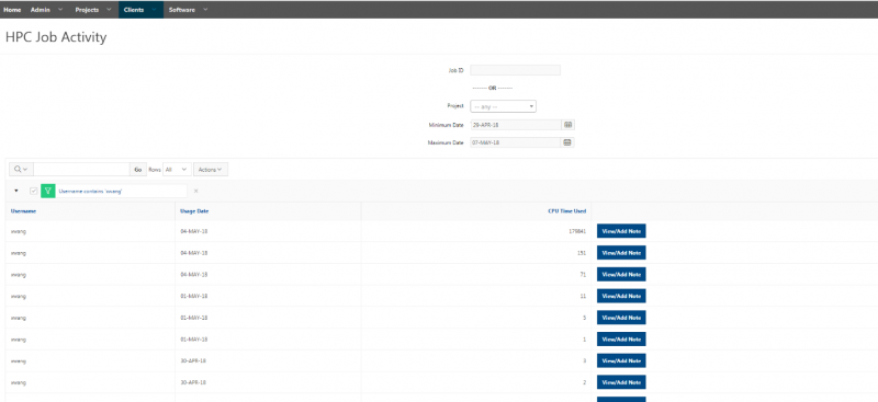
- To create a break group based on ‘Usage Date’, click ‘Actions -> Format -> Control Break’ as shown below:
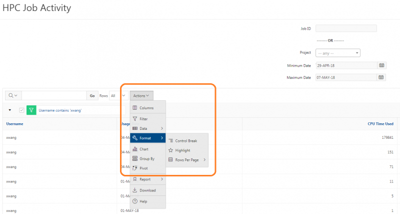
- You will get the ‘Control Break’ pop-up window. Choose ‘Usage Date’ under ‘Column’ with Status ‘Enabled’, as shown below:
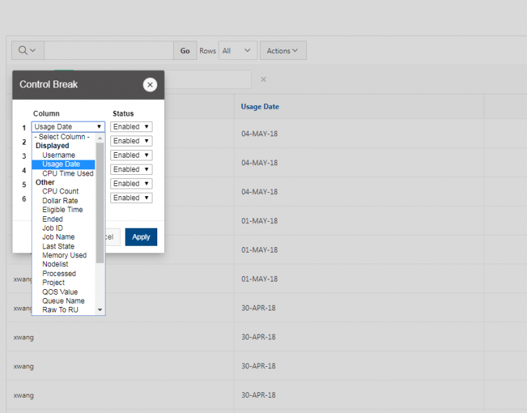
- Click ‘Apply’. This pulls the column ‘Usage Date’ out of the report and the jobs submitted by ‘xwang’ are grouped based on ‘Usage Date’, as shown below:
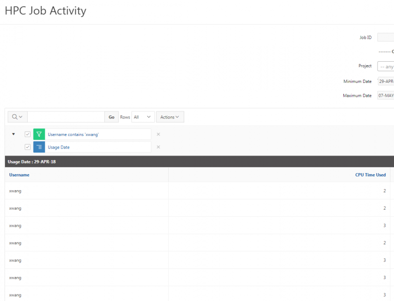
- To generate a chart report that shows the total CPU time per day, click ‘Actions -> Chart’ as shown below:
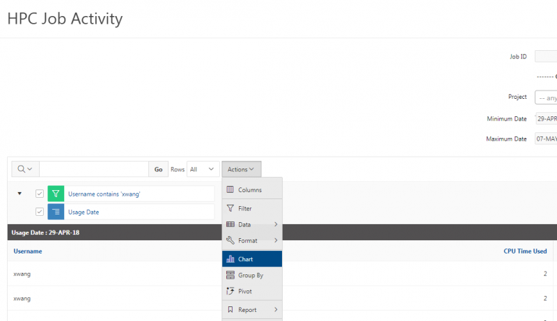
- You will get the ‘Chart’ pop-up window. Using the following information on the chart options, as shown in the image below:
- Chart Type: vertical bar
- Label: Usage Date
- Axis Title for Label: Date
- Value: CPU Time Used
- Axis Title for Value: Total CPU Time
- Function: Sum
- Sort: Default
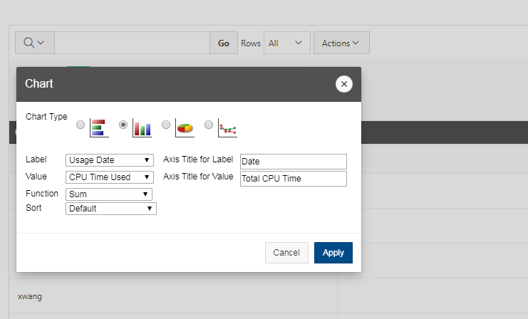
- Click the ‘Apply’ button. You will get the chart report showing the daily total CPU usage by ‘xwang’ between April 29, 2018 and May 7, 2018 (here, the CPU usage is zero if the date is missing in this chart):
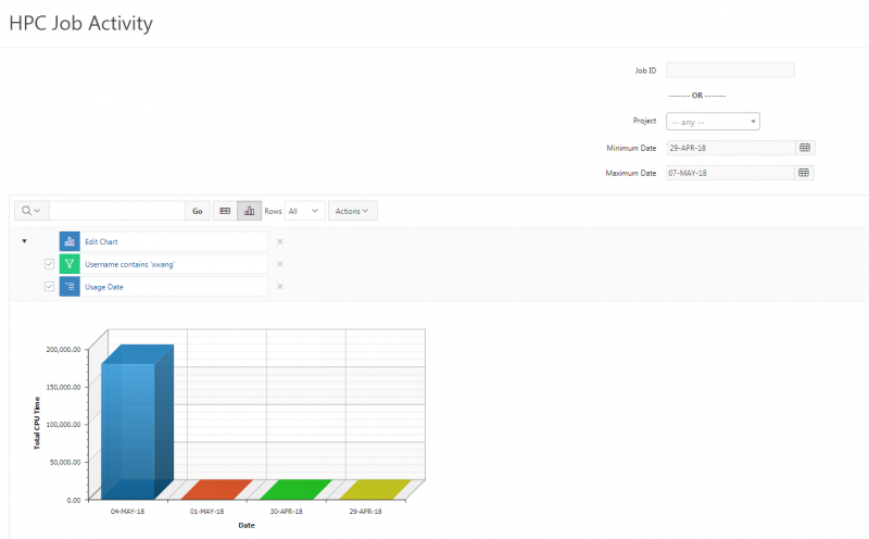
- From this chart, it is easy to see that ‘xwang’ used many CPU hours on May 4th, and very few CPU hours on other days. To switch back to report view, you can click the icon ‘View Report’ to the left of the row selection:
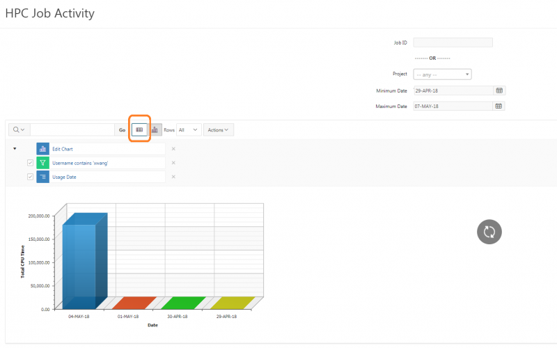
- You can save this report for future use by clicking ‘Actions -> Report -> Save Report’ as shown below:
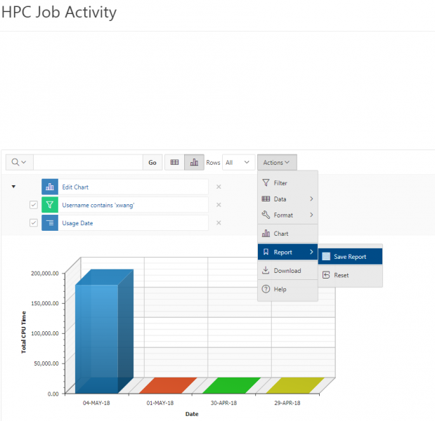
- You will get the ‘Save Report’ pop-up window. Provide ‘xwang Daily Usage’ as the name and ‘Daily CPU Usage between April 29 and May 07’ as Description, as below:
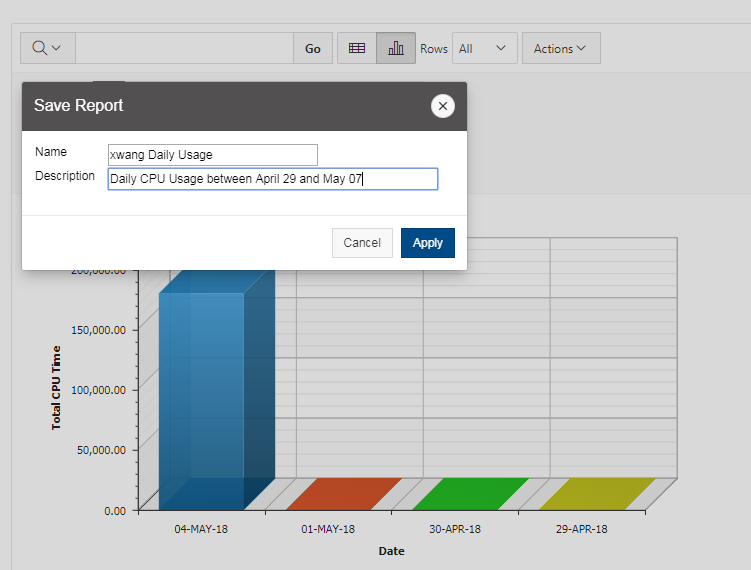
- Click ‘Apply’ button to save the report. Now, beside ‘Go’, you will be able to choose the reports between ‘Default -> Primary Report’ (which is the report that initially displays) and ‘Private -> xwang Daily Usage’, as shown below:
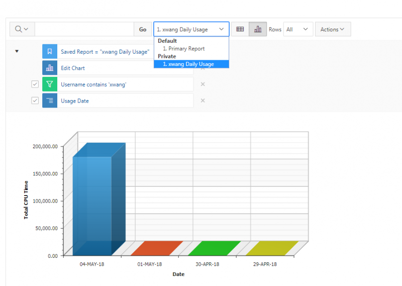
- For now, all customized reports are private, which means only the end user that created the report can view, save, rename or delete the report.
- You can download this report by clicking ‘Actions -> Download’ as shown below:
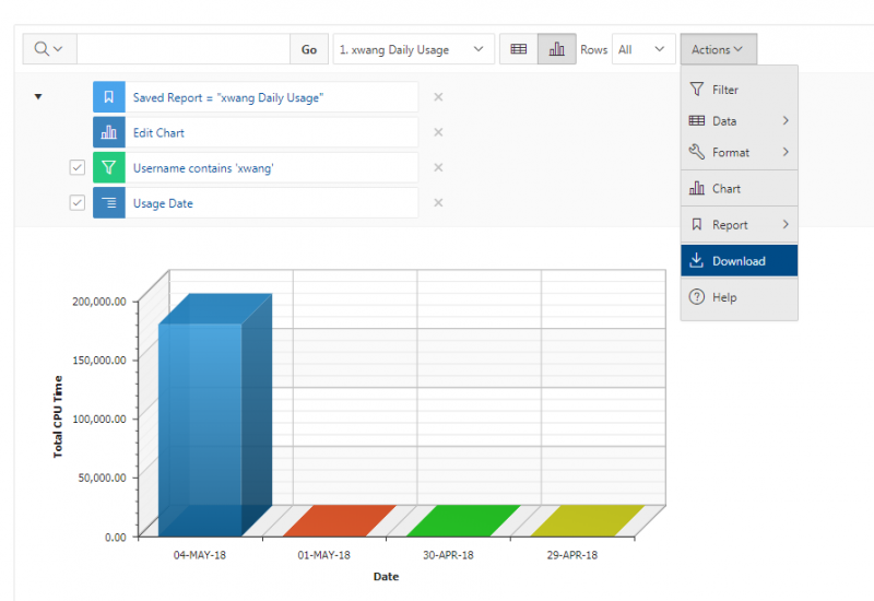
- You will get the ‘Download’ pop-up window as below:
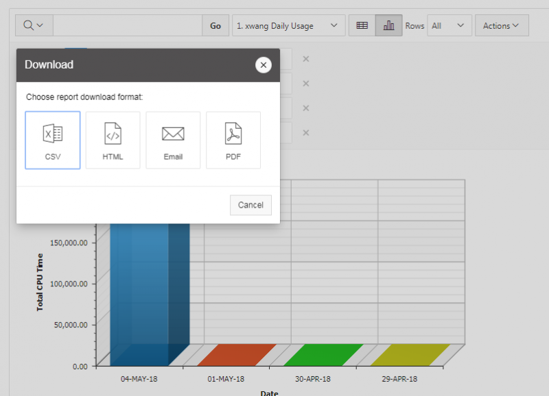
- Click the icon of CSV, HTML, or PDF to download this report, or click the icon of Email to email this report to the desired recipient. Please note the downloaded report is in the format of table only, while other formats like ‘Chart’ won’t be available for downloading.
Service:
OnDemand
OnDemand is our "one-stop shop" for access to our High Performance Computing resources. With OnDemand, you can upload and download files; create, edit, submit, and monitor jobs; run GUI applications; and connect via SSH, all via a web broswer, with no client software to install and configure.
We've created a brief video explaining OnDemand's capabilities so users can better gauge if it is the right fit for them. Getting connected to OnDemand is also covered in this video. In addition, we've developed tutorial videos for OnDemand's job client and file management client.
System Requirements
Currently, the site is confirmed to work with newer versions of Chrome (87+), Firefox (87+), and Internet Explorer (11+). We are still working to expand availability to additional clients and are planning on including compatibility for mobile devices (phones and tablets) in the future.
Connecting
To connect to OnDemand, visit https://ondemand.osc.edu. The first page of the OnDemand site displays instructions on how to log in to OSC OnDemand, which are shown in the image below:
There are two options for logging in.
Option 1: Using OSC HPC Credentials
Follow the steps below to use OSC HPC credentials to directly log in.
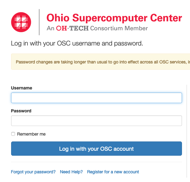
Option 2: Using Third-Party Credentials
You can also map third-party credentials to an OSC account and log in using the third-party credentials.
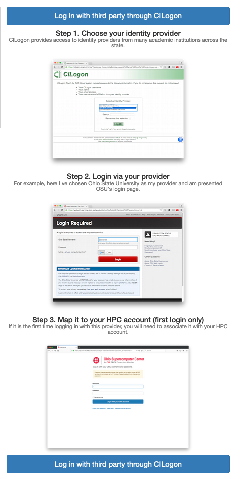
Click the button labeled "Log in with third party though CILogon" at the bottom to continue to step 1 shown below:
- Step 1 requires you to choose an identity provider to log in with. This can be any institute you're affiliated with or even services like Google.
If you check "Remember this selection" you will need to delete cookies from the cilogon domain to make a new choice. You can do this through your browser's settings or at https://cilogon.org/me - Step 2 has you log in using your credentials for the provider you picked.
- Step 3 has you log in with your OSC credentials in order to link your identity provider to your OSC account.
These three steps are only needed the first time you log in to OSC OnDemand.
Only one third-party credential can be mapped to an osc account at a time. An osc account can be disassociated from an external account by navigating to:
https://idp.osc.edu/realms/osc/account/identity
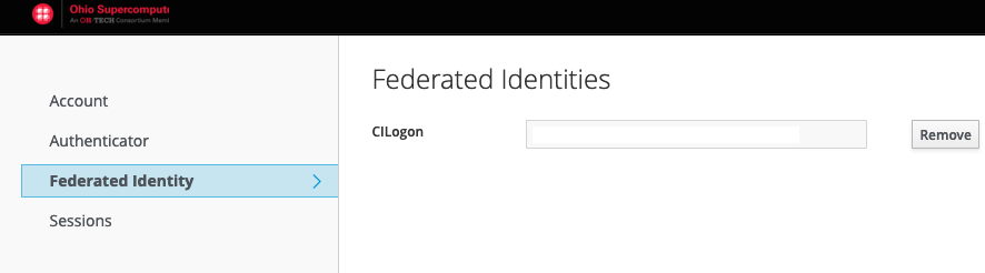
and clicking Remove.
Once completed you will be presented with this page:

Or this page if your browser window is more compact:

The three-lined icon to the right of the compact page expands when clicked to show the full toolbar that the non-compact page has. At this point, you can begin accessing the tools in OnDemand.
File Transfer
Move data on and off of OSC storage services. To use the file transfer client, select "Files" in the main menu. For more information, please visit the file transfer and management page.
Job Management
Create, edit, submit, and monitor jobs. To access the job management tools, use the "Jobs" menu. For more information about the tools, please visit the job management page.
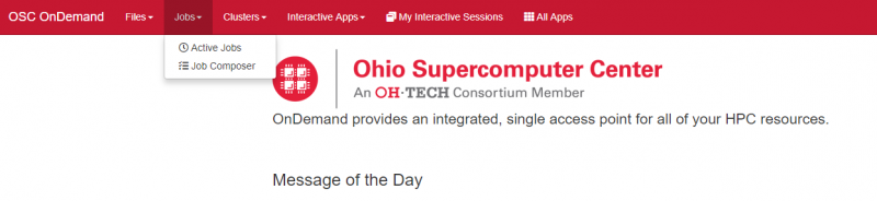
Shell Access
OnDemand provides the ability to SSH to Pitzer or Owens from inside your web browser. To get to a terminal, select the "Clusters" menu and choose either Pitzer or Owens.
Please note that this action will open a new tab with shell access to the cluster.
System Status
System status can be accessed by clicking on the "Clusters" tab and selecting "System Status" on the drop-down menu. This page shows the current status of the entire system (nodes in use, cores in use, and number of running, queued, and blocked jobs).
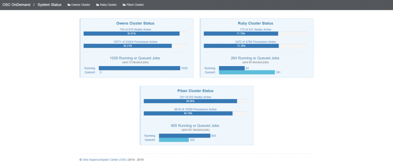
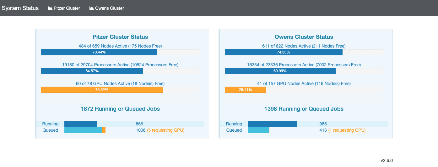
If you click the image, you'll get a detailed report including the total system load, the CPU usage, the total cluster memory use, and the total network traffic on the cluster. The "CPU Report" showing less than 100% use means that there are some cores not currently being used by a job, but that doesn't necessarily mean that they are available to be scheduled. There may be a system reservation that is preventing the scheduler from utilizing all of those cores.
Get a Virtual Desktop
Request a desktop to run GUI applications without the hassle or performance problems associated with X11 forwarding. To access one, please select either "Interactive HPC" or "Virtual Desktop Interface" from the "Desktops" menu.
Virtual Desktop Interface
Select one VDI app and you will arrive on the page shown below. Please modify the resolution information if needed and click "Launch." You may need to wait for a few minutes for the interface to launch.
The maximum walltime for VDI is 24 hours.
Here it also provides access to Files ("Access Files") and Shell (">_Launch Shell") and allows you to go back to the OnDemand main page ("Go to Dashboard").
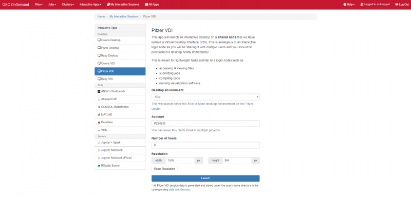
Once the interface is ready to be used, your session manager will have a job that looks like the image below:
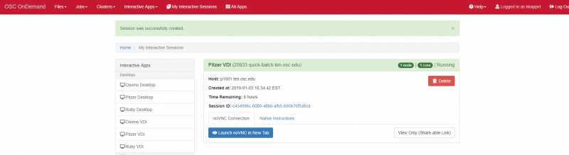
To access the interface, you can choose from "noVNC Instructions" or "Native Client Instructions." If you use "noVNC," you can choose from "Launch noVNC in New Tab" to get your desktop shown below and work accordingly, or "View Only (Shareable Link)" to get your desktop or share your desktop with colleagues in "View Only" mode. If you use "Native Client Instructions", see this page for more information on how to use OSC Connect.
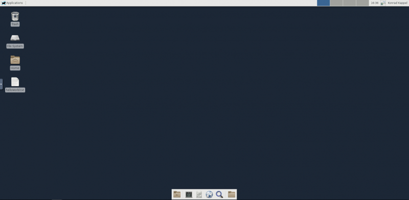
The Virtual Desktop Interfaces should not be used for computationally or memory intensive processes because it is a shared resource and there are other users on the same node. Such processes will be terminated. Please perform such work on compute node as discussed below.
Interactive HPC
Request a desktop on compute node through the batch system without the hassle or performance problems associated with X11 forwarding. To access one, please select "Pitzer Desktop" or others under "Interactive" from the "Desktops" menu.
If you choose "Pitzer Desktop," you will arrive on the page shown below. Please enter the information as desired and click "Launch." You may need to wait for a few minutes for the interface to launch. If you'd like to recieve an email notifiying you of when the interface has launched, please select "I would like to recieve an email when the session starts."
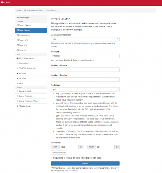
Once the interface is ready to be used, your session manager will have a job that looks like the image below:
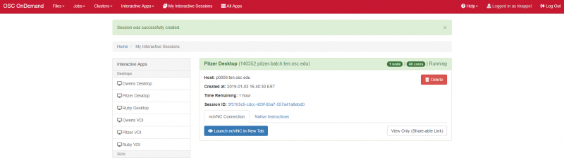
Similarly, you can choose from "noVNC Instructions" or "Native Client Instructions" to get the interface. If you use "noVNC," you can choose from "Launch noVNC in New Tab" to get your desktop and work accordingly, or "View Only (Shareable Link)" to get your desktop or share your desktop with colleagues in "View Only" mode. If you use "Native Client Instructions," see this page for more information on how to use OSC Connect.
Here you can run computationally or memory intensive processes since you do not share the node(s) with other clients.
Access Application on Compute Node
Request an application on compute node through the batch system without the hassle or performance problems associated with X11 forwarding. To access one, please select any app from the "Desktop Apps" menu. See "Desktop App Catalog" for more information.
Support Tickets
The OnDemand dashboard now supports the ability to send a support ticket to our Help Desk system.
To do so from your OnDemand Dashboard, simply go to > Help > Submit Support Ticket and fill in the following fields on the form that comes up:
Username: Logged in user. Username will be added to support ticket body for reference.
Email: Email address for communication regarding this ticket. Only a single email address is supported.
CC: Additional email address to copy onto this ticket. Only a single email address is supported.
Subject: Brief description of the problem.
Expected behavior: Detailed description of what was expected to happen.
Actual behavior: Detailed description of the unintended outcome.
Steps to reproduce: Detailed description of steps that led to the problem.
Service:
Desktop App Catalog
OSC OnDemand provides access to applications on compute nodes through the batch system, without the hassle or performance problems associated with X11 forwarding. To access one, please select an application under "Interactive HPC" from the "Desktop Apps" menu. For more information on each product, please go to its page provided below.
Supercomputer:
Service:
Accessing Parallel R tutorial
This document will guide you on how to launch Rstudio App and acess Parallel R workshop material through OSC onDemand.
Step 1: Log on to https://ondemand.osc.edu. Please see this guide on how to use OnDemand service.
Step 2: Launch Rstudio App
RStudio is an integrated development environment (IDE) for R. It includes a console, syntax-highlighting editor that supports direct code execution, as well as tools for plotting, history, debugging and workspace management.
Accessing through OnDemand
All the interactive apps can be found within the 'Interactive Apps' dropdown in our OnDemand web portal as shown in the image below:
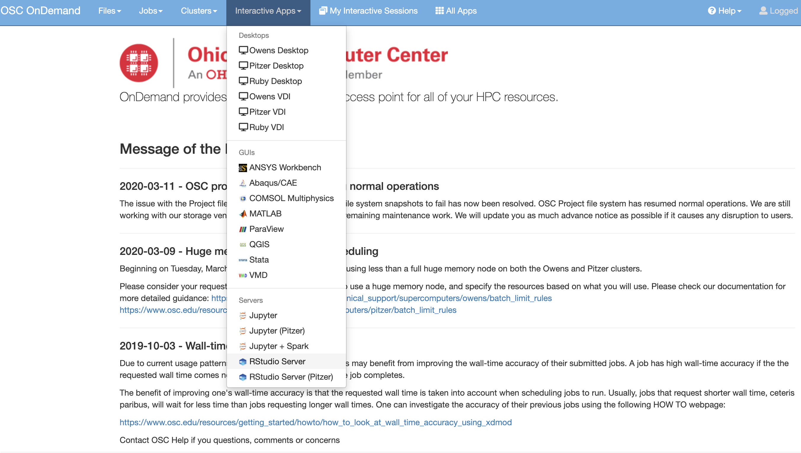
After selecting RStudio Server, you will arrive at this job submission page:
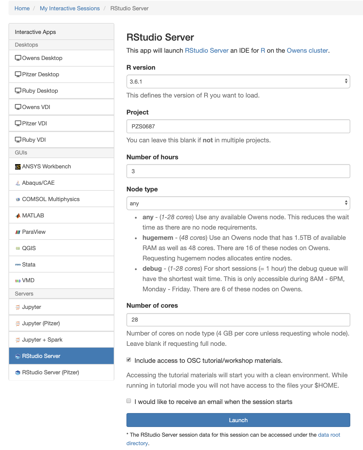
Here you can select the resources you would like your RStudio session to have using the menu on the lefthand side of the page. Please pick R/3.6.1 to access the tutorial material. Please provide your project ID as PZS0687 if you have registered for the workshop. If not, use your default project ID. Please contact oschelp@osc.edu if you dont have a project ID yet. Please make sure you check on the box that says Include access to OSC tutorial/workshop material. After you click "Launch", a new session will be queued. Once the session is active you page will look like the image below:
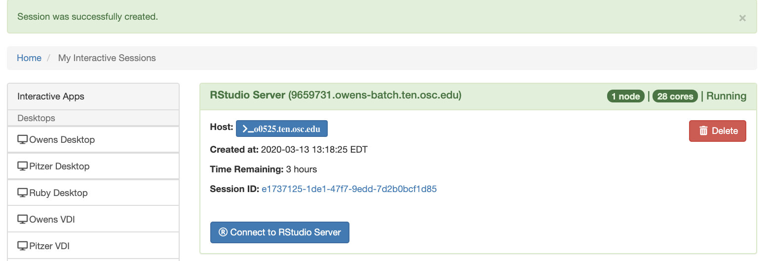
Click on "Connect to RStudio Server" to begin using RStudio.
Using RStudio
Once you have entered your session, you should see the RStudio page below:
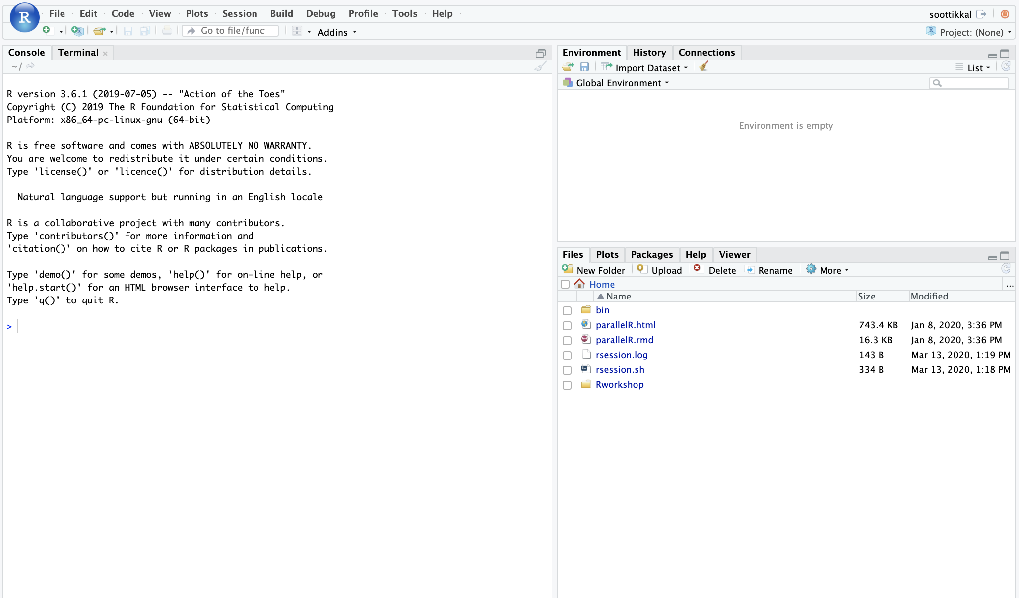
This is a typical RStudio interface that should be familiar to most users. Please note that Rstudio session for accessing the tutorial materials will start with a clean environment. While running in tutorial mode you will not have access to the files your $HOME.
- Top Left panel: code editer
- Bottom Left panel: The console where you can type commands and see the output.
- Top right panel:
- Environment tab: Shows all the active objects
- History tab: Shows a list of commands used so far.
- Bottom right panel:
- Files tab: Shows all the files and and folders in your home directory
- Plots tab: Shows all your graphs
- Packages tab: Lists a series of packages or add-ons needed to run certain processes
- Help tab: Can be used to find additional info
- Viewer tab: Used to view local web content
More info on RStudio and its use can be found on the RStudio official support page.
From the bottom right panel, please click on parallelR.rmd markdown file. This will open the training material in the code editer window as shown below.
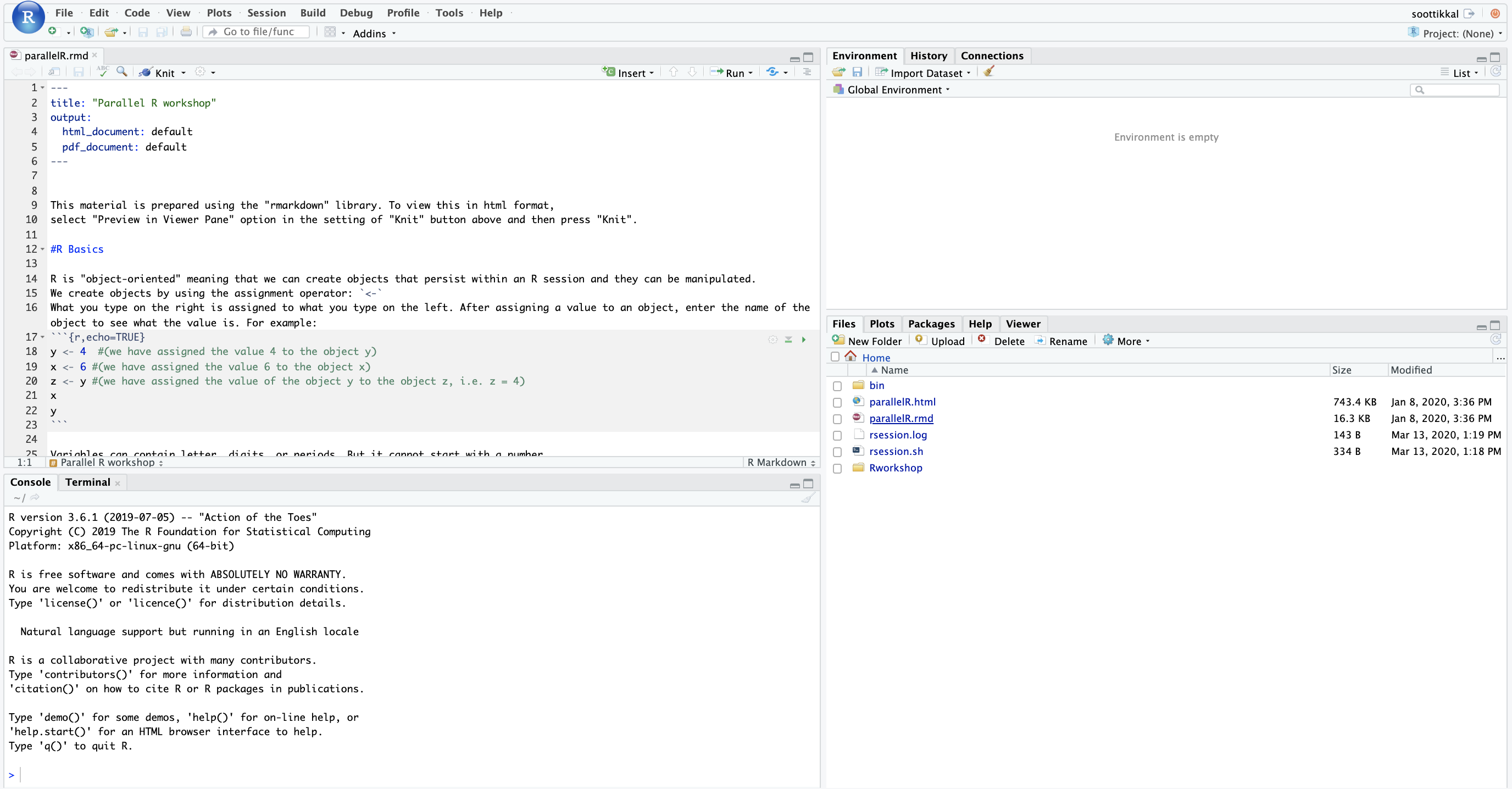
This ParallelR.rmd material is prepared using the “rmarkdown” library. To view this in html format, select “Preview in Viewer Pane” option in the setting of “Knit” button top of the code editer window and then press “Knit”.
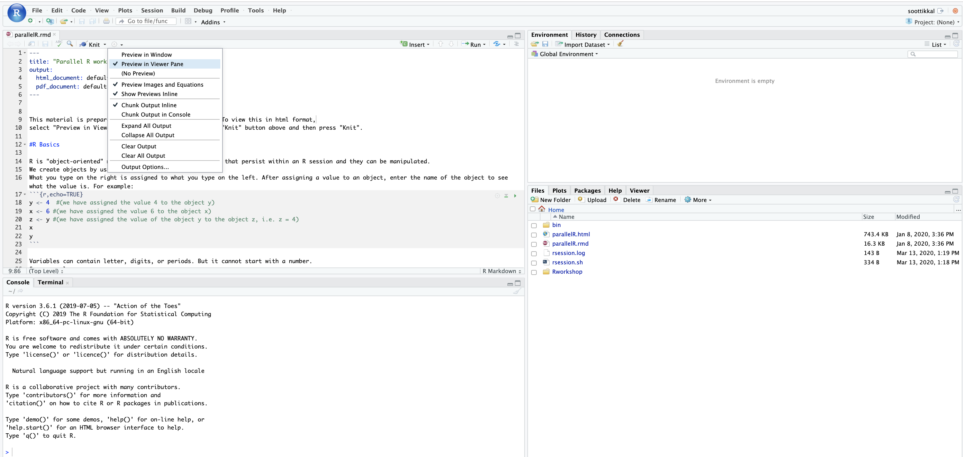
This will open html version of the rmd document in the Veiwer pane of bottom right panel.
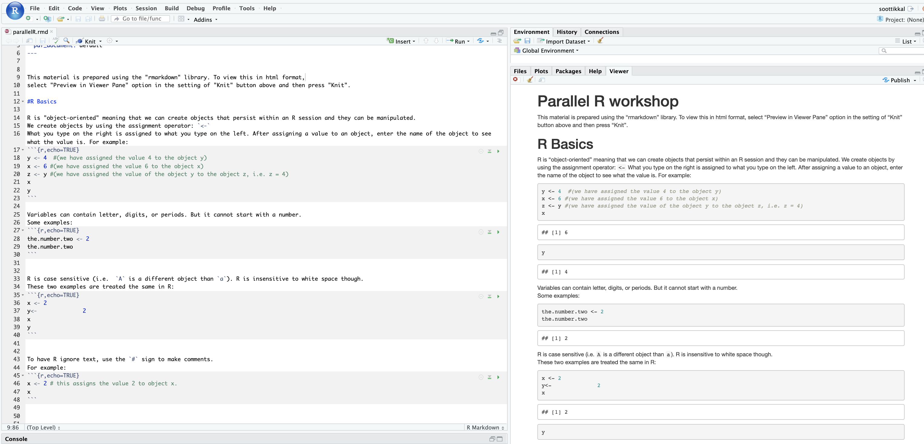
You can read though the html document in the Viewer Pane and execute codes in the Code editor. Press the Run/play button on the top right of each code block to run the code.
Please reachout to soottikkal@osc.edu if you have questions.
Supercomputer:
Service:
OnDemand Desktop App: MATLAB
MATLAB allows matrix manipulations, plotting of functions and data, implementation of algorithms, creation of user interfaces, and interfacing with programs written in other languages, including C, C++, C#, Java, Fortran and Python.
Accessing through OnDemand
All the desktop apps can be found within the 'Interactive Apps' dropdown in our OnDemand web portal as shown in the image below:
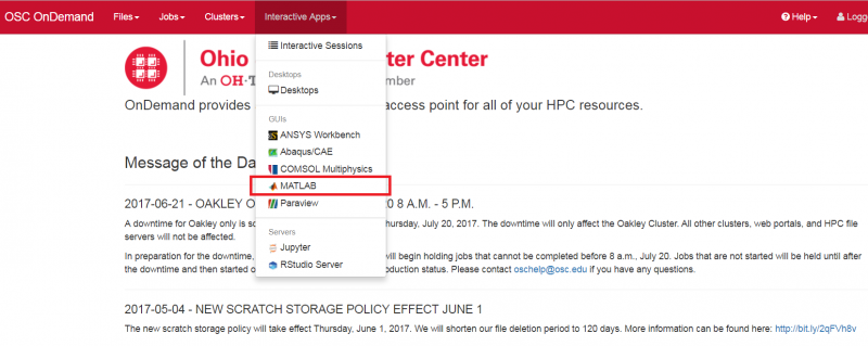
After selecting MATLAB, you will arrive at this page:
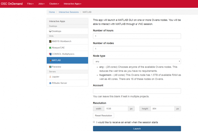
Here you can select the resources you would like your MATLAB session to have using the menu on the righthand side of the page. Additionally you can adjust the window size of the MATLAB session using the same menu. After you click "Launch", a new session will be queued. Once the session is active you page will look like the image below:
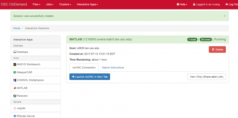
You can choose from "noVNC Connection", or "Native Instructions" to get the interface. If you use "noVNC", you can choose from "Launch noVNC in New Tab" to get your desktop and work accordingly, or "View Only (Share-able Link)" to get your desktop or share your desktop with colleagues in "View Only" mode. If you use "Native Instructions", see this page for more information on how to use OSC Connect.
Using MATLAB
Once you have entered your session, you should see a new tab. Allow MATLAB a moment to start up before your screen eventually looks like the image below:
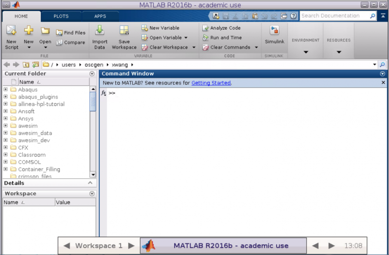
This is a typical MATLAB interface that should be familiar to most users.
The desktop includes these panels:
- Current Folder — Access your files.
- Command Window — Enter commands at the command line, indicated by the prompt (>>).
- Workspace — Explore data that you create or import from files.
More info on Matlab and its use can be found here.
Further Reading
Supercomputer:
Service:
OnDemand Desktop App: RStudio Server
RStudio is an integrated development environment (IDE) for R. It includes a console, syntax-highlighting editor that supports direct code execution, as well as tools for plotting, history, debugging and workspace management.
Accessing through OnDemand
All the desktop apps can be found within the 'Desktop Apps' dropdown in our OnDemand web portal as shown in the image below:
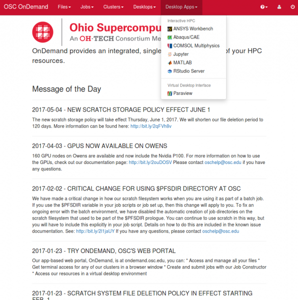
After selecting RStudio Server, you will arrive at this page:
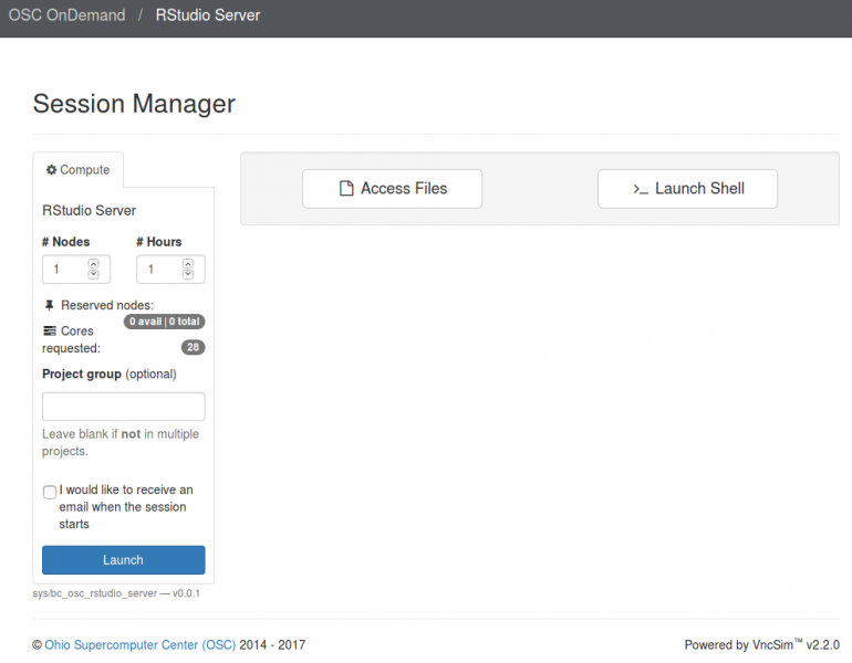
Here you can select the resources you would like your RStudio session to have using the menu on the lefthand side of the page. You can also access your files or launch the shell using the options in the center. After you click "Launch", a new session will be queued. Once the session is active you page will look like the image below:
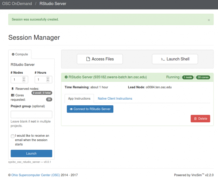
Click on "Connect to RStudio Server" to begin using RStudio.
Using RStudio
Once you have entered your session, you should see the RStudio page below:
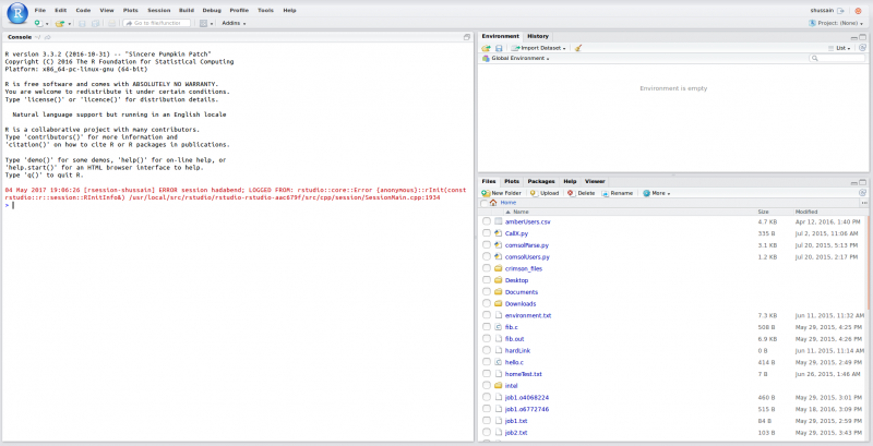
This is a typical RStudio interface that should be familiar to most users.
- Left panel: The console where you can type commands and see the output.
- Top right panel:
- Environment tab: Shows all the active objects
- History tab: Shows a list of commands used so far.
- Bottom right panel:
- Files tab: Shows all the files and and folders in your home directory
- Plots tab: Shows all your graphs
- Packages tab: Lists a series of packages or add-ons needed to run certain processes
- Help tab: Can be used to find additional info
- Viewer tab: Used to view local web content
More info on RStudio and its use can be found on the RStudio official support page.
Supercomputer:
Service:
File Transfer and Management
OnDemand provides a web-based File Explorer that can be used to upload and download files to your OSC home directory or project directory, and copy, delete, rename, and edit files.
Here is a tutorial video that gives a overview of OnDemand's file management client's capabilities and how to utilize them.
Here you can see a screen shot of what the main interface looks like.
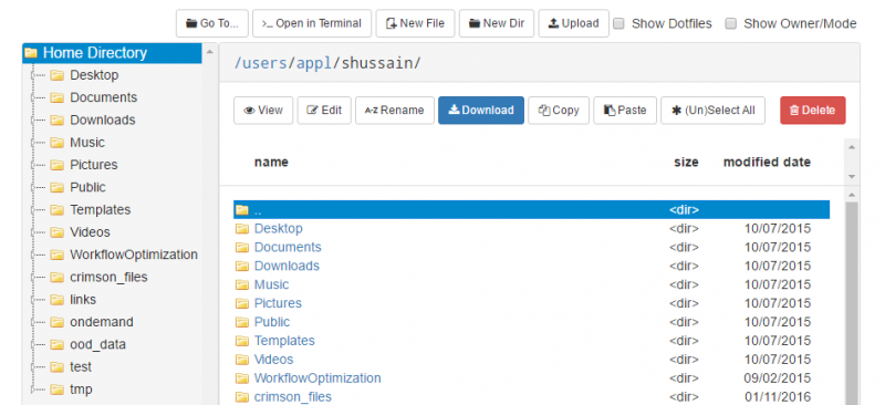
Navigating
Selecting which File System
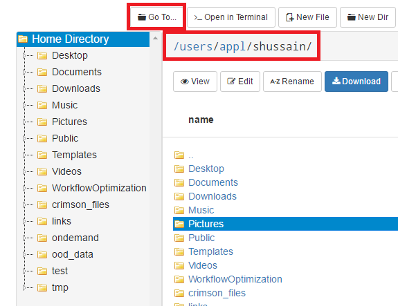
By default, the file browser will be looking at your home directory. If you have access to a project space for GPFS directory, you can switch to those by backtracking through the path near the top of the window and selecting the file system you wish to browse. In addition, you can use the "Go To" option in the top menu to type the path you wish to navigate to. Both the directory path and "Go To" button are highlighted in red in the image above.
Switching Folders
On the left side of the screen is a tree view of the directory structure. You can navigate this tree the same way you might on a normal desktop GUI to select the folder you wish to use.
Uploading and Downloading Files
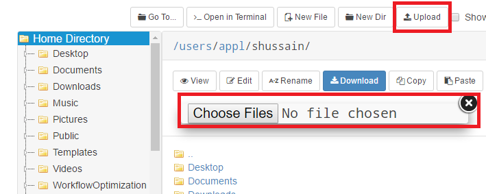
There are several methods to upload files. The first is to simply navigate to the desired destination, and then drag the file from your local desktop or window navigator to the OnDemand window. You can also click the "Upload" button to open a dialog that will allow you to navigate your local computer and select which files you want to upload. This process is highlighted in the image above.
To download files, you must select the file or files you wish to download, and then use the "Download" button. If you select multiple files ("control+click" or "shift+click") or a folder, the server will zip the files up and download a single zip archive to your desktop machine.
You can also click "Globus" to perform data transfer between OneDrive and other storage via Globus. See this Globus page for general information, and see this OneDrive in Globus on data transfer service with OneDrive.
There is a size limit for upload/download of data using ondemand file explorer of 10GB.
It is recommended to use an sftp client, globus, or command line tool such as rsync for larger data transfers.
Contact oschelp@osc.edu for questions and guidance.
It is recommended to use an sftp client, globus, or command line tool such as rsync for larger data transfers.
Contact oschelp@osc.edu for questions and guidance.
File Operations
Most file operations can be accomplished by selecting the file in the main window pane and selecting the desired operation from the main menu.
![]()
Viewing and/or Editing a File
The application also includes several built-in file editors. To access these editors and viewers, select the file you wish to view or edit, and select "Edit" from the main menu. This will open up a text editor in a new tab.
Service:
Job Management
OnDemand provides two related job managment tools: one allows you to create and submit jobs via your web browser, and the other allows you to monitor queued and running jobs.
Here is a tutorial video that gives an overview of OnDemand's Job client's capabilities and how to utilize them.

My Jobs
Selecting "My Jobs" in the Jobs menu will open an application that allows you to create new jobs and submit them to the cluster, and inspect the results of jobs submitted via this tool.
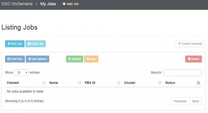
New Job
Please following the steps in order to create a job:
- Create a new job by copying from an existing job template directory (by clicking "+New Job" button under "Listing Jobs") or a previously run job directory (by clicking "+Copy Job" button under "Listing Jobs").
- If you click the "+New Job" button, you will see the page as below. Select the job template to copy, then click "Create New Job". The template directory will be copied and a new job row will be added to the top of the jobs table on the page titled "Listing Jobs"
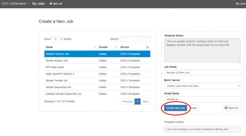
- If you click the "+New Job" button, you will see the page as below. Select the job template to copy, then click "Create New Job". The template directory will be copied and a new job row will be added to the top of the jobs table on the page titled "Listing Jobs"
- Select the job, then modify and/or add any files to this job by clicking "Edit Files"
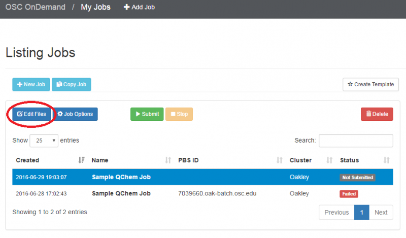
- Select the job and click "Job Options" to change the cluster, job name, or job script, if necessary
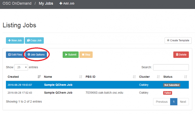
- At this point, you can submit the job using the green "submit" button from the "My Jobs" page; or return to this job later to modify it further. You can also monitor the job status here. Currently you must reload the page to see job status changes.
Job Management
On the main screen for "My Jobs" you can click on a job to examine it.
Submit Job
If the job has not been submitted, the "submit job" button will be active, and will submit the selected job to the queue.
Stop Job
The "stop" button will allow you to kill a running job.
Delete Job
The "delete" button will allow you to delete a job
Active Jobs
The "Active Jobs" application will show you all of jobs currently in the queue (running or queued), regardless of how the jobs were submitted. You can click the button on top to switch from:
- All jobs from your OSC account
- All jobs from your project/group
- All jobs from OSC users
You can also use "Search" tool to filter jobs based on sytems (oakley or ruby), status (running, queued, or hold), OSC user accout, etc.
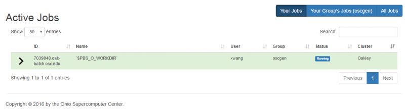
Job Inspection
If you click the arrow to the left of each job you can get more information about this job. It also provides the information of each node on which this job is running on, over the duration of the entire job. Clicking on each image expands it to show more information.
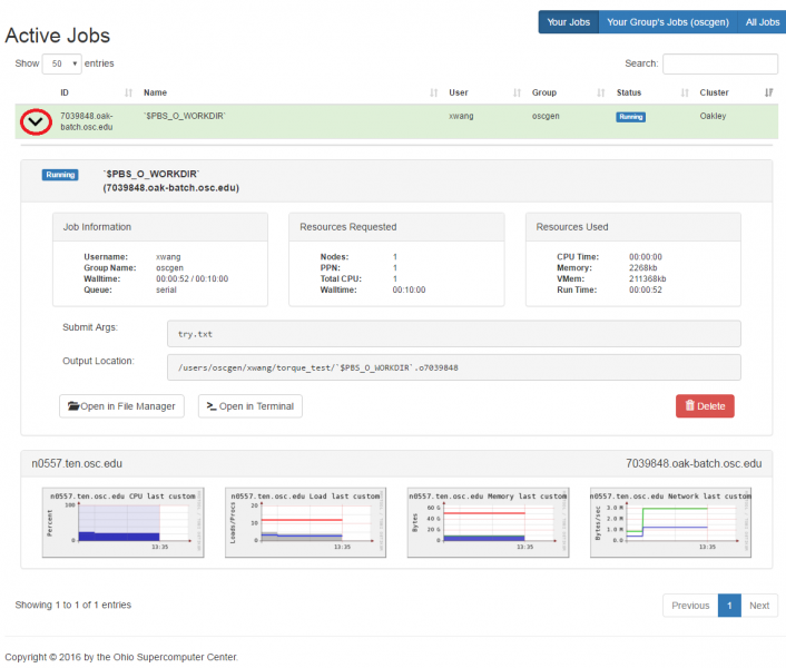
Service:
Facilitation
A key component of our client resources is devoted to facilitation in order to ensure Ohio Supercomputer Center (OSC) users gain the full benefits of our high performance computing (HPC) services as efficiently as possible without being bogged down in the inner-workings of complex computations.
Our facilitators focus on a number of tasks essential to providing OSC services to Ohio’s academic and industrial research communities:
Research Support
OSC staff works closely with research to understand their projects and goals. This allows our team members to evaluate our users’ needs and recommend the best solutions for gaining full access to our resources. Facilitators can pinpoint key areas in which a user may need a better understanding of what OSC offers, helping them develop a full plan for the implementation of our resources based on their needs.
Education and Training
HPC and networking resources come together at OSC to create an exciting and innovative teaching and research environment. And, through the integration of increased training and education leadership over the past year, OSC is working toward deeper engagement with our users. OSC staff members assist faculty and student researchers by providing workshops, one-on-one classes, web-based training and materials. Our education and training outreach includes:
- On-site instruction workshops
- Campus visits
- Classroom accounts
- XSEDE training
- Faculty Recruitment
- Our 24/7 Help Desk
Outreach
OSC staff regularly work to raise the awareness and understanding of our available services to both the academic and industrial communities looking to leverage high performance computing in research.
Data Storage
OSC has various storage systems to fulfill different HPC research needs. Information on the each filesystem can be found in data storage technical documentation.
Data storage overview and documentation
Review the overview of the filesystems, storage hardware, and the storage documentation.
Protected data service
Review information about storing data with strict security needs.
Data storage upgrades
OSC's data storage is continually updated and expanded. View the some of the major changes.
Known issues of OSC filesystems
Visit known issues and filter by the filesystem category to view current known issues with filesystems.
Overview of File Systems
OSC has several different file systems where you can create files and directories. The characteristics of those systems and the policies associated with them determine their suitability for any particular purpose. This section describes the characteristics and policies that you should take into consideration in selecting a file system to use.
The various file systems are described in subsequent sections.
Visibility
Most of our file systems are shared. Directories and files on the shared file systems are accessible from all OSC HPC systems. By contrast, local storage is visible only on the node it is located on. Each compute node has a local disk with scratch file space.
Permanence
Some of our storage environments are intended for long-term storage; files are never deleted by the system or OSC staff. Some are intended as scratch space, with files deleted as soon as the associated job exits. Others fall somewhere in between, with expected data lifetimes of a few months to a couple of years.
Backup policies
Some of the file systems are backed up to tape; some are considered temporary storage and are not backed up. Backup schedules differ for different systems.
In no case do we make an absolute guarantee about our ability to recover data. Please read the official OSC data management policies for details. That said, we have never lost backed-up data and have rarely had an accidental loss of non-backed-up data.
Size/Quota
The permanent (backed-up) and scratch file systems all have quotas limiting the amount of file space and the number of files that each user or group can use. Your usage and quota information are displayed every time you log in to one of our HPC systems. You can also check your home directory quota using the quota command. We encourage you to pay attention to these numbers because your file operations, and probably your compute jobs, will fail if you exceed them. If you have extremely large files, you will have to pay attention to the amount of local file space available on different compute nodes.
Performance
File systems have different performance characteristics including read/write speeds and behavior under heavy load. Performance matters a lot if you have I/O-intensive jobs. Choosing the right file system can have a significant impact on the speed and efficiency of your computations. You should never do heavy I/O in your home or project directories, for example.
Table overview
Each file system is configured differently to serve a different purpose:
| Home Directory | Project | Local Disk | Scratch (global) | Backup | |
|---|---|---|---|---|---|
| Path | /users/project/userID |
/fs/ess |
/tmp |
/fs/scratch |
N/A |
| Environment Variable | $HOME or ~ | N/A | $TMPDIR | $PFSDIR | N/A |
| Space Purpose | Permanent storage | Long-term storage | Temporary | Temporary | Backup; replicated in Cleveland
|
| Backed Up? | Daily | Daily | No | No | Yes |
| Flushed | No | No | End of job when $TMPDIR is used |
End of job when $PFSDIR is used |
No |
| Visibility | Login and compute nodes | Login and compute nodes | Compute node | Login and compute nodes | N/A |
| Quota/Allocation | 500 GB of storage and 1,000,000 files | Typically 1-5 TB of storage and 100,000 files per TB. | Varies. Depending on node | 100 TB of storage and 25,000,000 files | N/A |
| Total Size | 1.9 PB |
/fs/ess: 13.5 PB |
Varies. Depending on system |
/fs/scratch: 3.5 PB |
|
| Bandwidth | 40 GB/S |
Reads: 60 GB/S Writes: 50 GB/S |
Varies. Depending on system | Reads: 170 GB/S
Writes: 70 GB/S |
N/A |
| Type | NetApp WAFL service | GPFS | Varies. Depending on system | GPFS |
Service:
Storage Hardware
The storage at OSC consists of servers, data storage subsystems, and networks providing a number of storage services to OSC HPC systems. The current configuration consists of:
- A NetApp Network Attached Storage (NAS) for home directories (1.9 PB of storage, 40 GB/s bandwidth)
- An IBM Elastic Scale System (ESS) to provide project and scratch storage, and add support for various protected data requirements (~16 PB of storage, bandwidth varies depending on Project and Scratch)
- Local disk storage on each compute node
- Two IBM tape robots for backups and archival which as of the beginning of 2022:
- Capable of redundantly storing up to 23.5 PB of data, with copies kept both in Columbus and Cleveland area data centers.
- Has nearly 14 PB of tapes installed in the tape backup archive, with several additional PB of tapes on hand ready to be installed as needed
- Anticipated to be scalable via new generations of tape media and drives to over 141 PB of capacity in the coming years
Service:
2016 Storage Service Upgrades
On July 12th, 2016 OSC migrated its old GPFS and Lustre filesystems to new Project and Scratch services, respectively. We've moved 1.22 PB of data, and the new capacities are 3.4 PB for Project, and 1.1 PB for Scratch. If you store data on these services, there are a few important details to note.
Paths have changed
The Project service is now available at /fs/project, and the Scratch service is available at /fs/scratch. We have created symlinks on the Oakley and Ruby clusters to ensure that existing job scripts continue to function; however the symlinks will not be available on future systems, such as Owens. No action is required on your part to continue using your existing job scripts on current clusters.
However, you may wish to start updating your paths accordingly, in preparation for Owens being available later this year.
Data migration details
Project space allocations and Scratch space data was migrated automatically to the new services. For data on the Project service, ACLs, Xattrs, and Atimes were all preserved. However, Xattrs were not preserved for data on the Scratch service.
Additionally, Biomedical Informatics at The Ohio State University had some data moved from a temporary location to its permanent location on the Project service. We had prepared for this, and already provided symlinks so that the data appeared to be in the final location prior to the July 12th downtime, so the move should be mostly transparent to users. However, ALCs, Xattrs, and Atimes were not preserved for this data.
|
File system |
Transfer method |
ACLs preserved |
Xattrs preserved |
Atime preserved |
|
/fs/project |
AFM |
Yes |
Yes |
Yes |
|
/fs/lustre |
rsync |
Yes |
No |
Yes |
|
/users/bmi |
rsync |
No |
No |
No |
Full documentation
Full details and documentation of the new service capacities and capabilities are available at https://www.osc.edu/supercomputing/storage-environment-at-osc/
Service:
2020 Storage Service Upgrades
In March 2020, OSC expanded the existing project and scratch storage filesystems by 8.6 petabytes. Adding the existing storage capacity at OSC, this brings the total storage capacity of OSC to ~14 petabytes.
A petabyte is equivalent to 1,024 terabytes.
New file paths
The new project and scratch storage is available using the path /fs/ess/<project-code> for project space and /fs/ess/scratch/<project-code> for scratch space. Existing data can be reached using the existing paths /fs/project and /fs/scratch.
New project storage allocation requests
Any new project storage allocation requests will be granted on the new storage, as long as the project did not have existing project space. Any new storage allocations will use the file path /fs/ess/<project-code>.
Some projects will have access to the new scratch space at /fs/ess/scratch/<project-code>. We will work with the individual group if access to /fs/ess/scratch/ is granted for that group.
Migrating storage
Existing project and scratch storage space may be required to move to the new storage space. If this happens, then OSC can optionally setup a symlink or a redirect, so that compatibility for programs and job scripts is maintained for some time. However, redirects are not a permanent solution and will be removed after some time. The members of the project should work to make sure that once the redirect is removed, it does not negatively affect their work at OSC.
Service:
2022 Storage Service Upgrades
In October 2022, OSC retires the Data Direct Networks (DDN) GRIDScaler system deployed in 2016 and expands the IBM Elastic Storage System (ESS) for both Project and global Scratch services. This expands the total capacity of Project and Scratch storage at OSC to ~16 petabytes with better performance.
A petabyte is equivalent to 1,024 terabytes.
File paths
All project and scratch storage is available using the path /fs/ess/<project-code> for project space and /fs/scratch/<project-code> for scratch space.
Migrating storage
OSC have been migrating all current Project data and Scratch data to the new services since September 2022, and runs the final synchronization of the data during Oct 11 2022 downtime. ACLs and extended attributes for the data are also preserved after the migration.
During December 13 2022 downtime, OSC cleaned the scratch directories for users who used to have scratch on both DDN and ESS storage (/fs/scratch/<project-code>and /fs/ess/scratch/<project-code>). All directories under /fs/ess/scratch/ points to /fs/scratch/ so they are essentially the same storage.
OSC have setup symlinks for the data on the storage so the compatibility for programs and job scripts is maintained. Please start to update your existing scripts to replace /fs/project/<project-code> with /fs/ess/<project-code> for project; and replace /fs/ess/scratch/<project-code> with /fs/scratch/<project-code> for scratch.
We encourage you to use
/fs/ess/<project-code> for project storage and /fs/scratch/<project-code> for scratch storage in all future job scripts.Directories from OnDemand Files App
For users who used to have project space on the DDN storage, you will see /fs/ess/<project-code> instead of /fs/project/<project-code>. Please use the directory /fs/ess/<project-code> , which is your current project space location including all of your previous data on project.
For users who used to have scratch on the ESS storage, you will see /fs/scratch/<project-code instead of /fs/ess/scratch/<project-code>). Please use the directory /fs/scratch/<project-code, which is your current scratch space location including all of your scratch data.
Service:
Protected Data Service
OSC's Protected Data Service (PDS) is designed to address the most common security control requirements encountered by researchers while also reducing the workload on individual PIs and research teams to satisfy these requirements.
Protected Data at OSC
The OSC cybersecurity program is based upon the National Institute of Standards and Technology (NIST) Special Publication (SP) 800-53, Revision 4 requirements for security, and reflects the additional requirements of established Information Technology (IT) security practices.
OSC currently supports the following protected data types.
- Personal Health Information (PHI)
- data covered by Health Insurance Portability and Accountability Act (HIPAA)
- Research Health Information (RHI)
- Export Control data
- International Traffic in Arms Regulations (ITAR)
- Export Administration Regulations (EAR)
- Personally Identifiable Information (PII)
- Proprietary Data
If you need support for a data type that is not listed, please contact OSC Help to discuss.
OSC only provides support for unclassified data processing, regardless of the specific category of that information. No support for data classified at secret or above is provided, and researchers should not, under any circumstance, transfer such data to OSC systems.
Getting started with the Protected Data Service at OSC
OSC's PDS was developed with the intent of meeting the security control requirements of your research agreements and to eliminate the burden placed on PIs who would otherwise be required to maintain their own compliance infrastructure with certification and reporting requirements.
In order to begin a project at OSC with data protection requirements, please follow these steps:
Contact OSC
Send an email to oschelp@osc.edu and describe the project's data requirements.
Consultation
You will hear back from OSC to set up an initial consultation to discuss your project and your data. Based on your project and the data being used, we may request the necessary documentation (data use agreements, BAA, MOU, etc).
Approval
Once OSC receives the necessary documentation, the request to store data on the PDS will be reviewed, and if appropriate, approved.
All PDS projects require multi-factor authentication (MFA). MFA will be set by OSC when the project is created.
Get started
OSC will help set up the project and the storage used to store the projected data. Here is a list of useful links:
- Getting started documentation: the guidance on how to start research for all new users
- PDS acceptable use and guidance document: Users are expected to comply with the guidelines in this document when working with PDS at OSC
- Manage the protected data and its access: the guidance on how to manage the projected data in the location with right permissions, as well as the access to the data
- Securely transferring files: the guidance on how to transfer proteced data
Manage the protected data and its access
Keep protected data in proper locations
Protected data must be stored in predetermined locations. The only locations at OSC to store protected data are
(Only with prior approval from OSC may a protected data service project not have a project prefix of PDE).
/fs/ess/PDEXXXX and /fs/scratch/PDEXXXX directories.(Only with prior approval from OSC may a protected data service project not have a project prefix of PDE).
There are other storage locations at OSC, but none of the follwing locations can be used to store protected data because they do not have the proper controls and requirements to safely store it:
/users/<project-code>/fs/ess/<non-PDS-project>/fs/scratch/<non-PDS-project>
PDS is the acronym for Protected Data Service.
Project space access controls and permissions should not be altered
The directory permissions where protected data are stored are setup to prevent changing the permissions or access control entries on the top-level directories by regular users. Only members of the project are authorized to access the data; users are not permitted to attempt to share data with unauthroized users.
The protected data environment will be monitored for unauthorized changes to permissions and access control.
Grant and remove user access to protected data
Protected data directoires will be set with permissions to restrict access to only project users. Project users are determined by group membership. For example, project PDE1234 has a protected data location at /fs/ess/PDE1234 and only users in the group PDE1234 may access data in that directory.
Adding a user to a project in OSC client portal adds the group to their user account, likewise removing the user from the project, removes their group. See our page for invite, add, remove users.
A user's first project cannot be the secure data project. If a user's first project was the secure data project, then removing them from the project in client portal will not take away their group for that project.
Keep accounts secure
Do not share accounts/passwords, ever.
A user that logs in with another person's account is able to perform actions on behalf of that person, including unauthorized actions mentioned above.
Securely transferring files to protected data location
Securely transferring files at OSC
Files containing personal health information (PHI) must be encrypted when they are stored (at rest) and when they are transferred between networked systems (in transit).
Transferring files securely to OSC involves understanding which commands/applications to use and which directory to use.
Before transferring files, one should ensure that the proper permissions will be applied once transferred, such as verifying the permissions and acl of the destination directory for a transferred file.
FileZilla
Install filezilla client software and use the filezilla tutorial to transfer files.
Use the client sftp://sftp.osc.edu
Select login type as interactive, as multi-factor authentication will be required to login for protected data projects.
Make sure to use sftp option
It is connected to user's home directory by default.
Need to navigate to
It is connected to user's home directory by default.
Need to navigate to
/fs/ess/secure_dir before starting the file transferGlobus
There is guide for using globus on our globus page.
Protected Data Service projects must use the OSC high assurance endpoint or transfers may fail. Ensure protected data is being shared in accordance with its requirements.
Command-line transfers
Files and directories can also be transferred manually on the command line.
secure copy (scp)
scp src <username>@sftp.osc.edu:/fs/ess/secure_dir
sftp
sftp <username>@sftp.osc.edu ## then run sftp transfer commands (get, put, etc.)
rsync
rsync --progress -r local-dir <username>@sftp.osc.edu:/fs/ess/secure_dir
Security, Accessibility, and Policies
Cybersecurity Audits:
OSC is regularly audited for alignment with the NIST SP 800-53 and ISO27002 security standards (see security framework for details) and has completed the HECVAT version 3.0. OSC has a general process for responding to client requests for more details or to fill out specific security questionnaires, as follows:
- OSC and the client must execute an NDA/CDA
- OSC can then share summary reports from existing audits and/or completed industry standard questionnaires
- If client wants a specific security questionnaire completed, client must first execute a computational services agreement with OSC, committing them to an initial $250 project fee
- OSC will utilize that fee evaluate / complete the questionnaire utilized up to 2 hours of staff time. If additional time is required to fully complete it, OSC will provide the partially completed questionnaire to the client along with a cost estimate of how much additional time at $100 / hour will be required to fully complete it.
- If the client approves of the cost estimate, OSC will fully complete the questionnaire and apply the charge to the next monthly bill
Export Controlled Projects:
OSC regularly hosts export controlled / ITAR / EAR projects and handles the corresponding code and/or data on all of OSC's available resources. Oversight of this is by the Ohio State Office of Secure Research and is covered by a Facility Control Plan (FCP) and Technology Control Plans (TCPs) as appropriate. Currently, there is no surcharge for export controlled projects compared to OSC's regular costs. OSC does NOT currently support CUI projects / code / date, but is evaluating those requirements for potential future compliance.
It is the responsibility of the PI of a project to inform OSC whether their project will contain any of these data types and whether that data requires special access controls.
HIPAA Projects:
OSC is piloting support for HIPAA / PHI / PII projects and the corresponding code and/or data with its protected data service. Please contact OSC Help using the information below for more details.
It is the responsibility of the PI of a project to inform OSC whether their project will contain any of these data types and whether that data requires special access controls.
Digital Accessibility:
OSC, as part of The Ohio State University, is committed to ensuring that all constituents can access digital information and digital services. OSC abides by the OSU policies regarding this.
Websites: OSC clients can make use of OSC resources using a variety of tools and software. The OnDemand.osc.edu and my.osc.edu websites are the preferred interfaces, but everything a client can do there can do via other mechanisms as well, such as traditional command line connections or via the OSC help desk. These websites are regularly evaluated using digital accessibility tools such as Axe, Lighthouse, and NVDA. OSC also hosts a variety of software packages and applications from external vendors, but can not guarantee the digitial accessibility status of each of them.
Events: OSC has provisions to provide live captioning or interpretation, upon request, for any events that OSC coordinates, such as training classes or workshops.
Questions or requests regarding digital accessibilty for any of OSC's resources or services can be directed to OSC help using the contact info below.
Specific Policy Documents:
Here are links to our current policies:
| Services | Link to the policy |
|---|---|
| Compute | Job walltime extension policy |
| Storage | Home storage policy |
| Project policy | |
| Scratch policy |
Policies that are in process of being updated can be found under proposed policies open for public comment.
If you have further questions on any of these topics, please contact OSC Help using the contact info below:
Phone: (614) 292-1800
Email: oschelp@osc.edu
Proposed OSC Policies for Public Comments
This page lists all proposed OSC policies for public comments. Your comments help inform our policies and are encouraged. We will provide the response to comments on this webpage after the public comment period closes. Please submit your comments via our online form by the deadline.
Currently Open for Public Comment:
Service:
Service Costs
Client Categories
The Ohio Supercomputer Center provides services to clients from a variety of types of organizations. The service costs and business models are different between Ohio-based academic clients and everyone else.
Ohio academic clients
Reflecting OSC’s founding as an academic computing resource, a majority of OSC’s users are Ohio-based and academic, including individuals engaged in both research and teaching. Classroom usage is always free and academic researchers in Ohio qualify for credits that largely or completely offset fees. See the Ohio Academic Fees FAQ and General Services FAQ sections below for more details.
Commercial, nonprofit and more
OSC services are available to anyone, anywhere. Commercial/nonprofit clients purchase services at set rates. These clients include businesses, nonprofits, government agencies, hospitals and health care, and academic institutions outside of Ohio.
Commercial/nonprofit clients must sign a service agreement, provide a $500 deposit and pay for resource usage. In most cases, clients in this category must purchase licenses to use commercial software packages provided by OSC. Details are available below in the General Services FAQ section.
Contact us for more details about the rates and to start the process of signing a service agreement.
Services Offered
The Ohio Supercomputer Center offers a range of services for clients of all types. These include:
Premium Compute
Access OSC’s clusters at low rates based on client category and node type/GPU, charged per core-hour used. This is our most popular service type.
Dedicated Compute
Prepay for secure priority access to specific types and quantities of nodes for multiple years. Fees are based on the specific node types selected and their quantity. Also known as “condo” service.
Project Storage
For projects with storage requirements that exceed home directory limits (500gb), OSC’s large-scale Project Storage service is available upon request at low costs.
Consulting Expertise
OSC staff provide routine technical support and expertise to clients at no cost. More advanced or lengthy engagements with our versatile specialists and engineers may be established at reasonable rates based on the scope of the project.
OSC also provides Protected Data Service, charged at the same rate, that allows for the use of certain categories of data, such as PHI, HIPAA. See this Protected Data Service page for more information.
General Services FAQ
Click on a question below to read more.
What is the relationship between the service costs for each client category?
The Ohio academic fees have no direct impact on other clients or the rates they are charged. Clients that are NOT based at Ohio academic institutions account for about 10 percent of usage of OSC resources, and the income derived from their usage helps fund the Center’s operating budget. While OSC charges them rates significantly higher than those charged to Ohio-based academic clients, OSC strives to keep its pricing competitive in the market.
How can clients allocate job costs to different funding sources?
Clients can be associated with multiple projects so that they can indicate at the time of submission which projects a job charge should apply to. The dashboard info a client sees in OnDemand has info broken down by projects and this project-level usage is detailed in the billing to the institutions. You could also use charge accounts to group multiple projects under the same funding source together for billing purposes, as seen in the billing statement. Another approach is to encode information in the job name. Clients can then log on to my.osc.edu and are able to run reports that group things by job name patterns. Finally, there is an ‘add note’ field available in my.osc.edu for each job that allows clients to add notes after a job has run (and hence then filter/sort by those notes).
Can clients tell day by day what their current compute charges are?
Each project in my.osc.edu will have a ‘budget balance’ display that is updated automatically each day and tells clients how much dollar balance is remaining on the project out of the budget you set, not including queued or running jobs. Certain types of clients are allowed to associate an 'unlimited' budget to projects to make them 'unbudgeted' if needed. In addition, it’s possible to run reports in my.osc.edu for any custom time frame showing all the jobs run in that time period and their corresponding charges. You can check your usage and cost yourself by following the instructions here.
Can non-Ohio-academic clients use budgets to control service consumption?
Yes! OSC can set budgets on your behalf to constrain any of your projects, similar to how Ohio Academic clients are required to constrain usage. Please contact your business relationship manager or email OSCHelp@osc.edu for assistance.
How do these rates compare to the costs a client would incur using another service?
OSC has done extensive cost comparisons between our rates and comparable services such as commercial cloud providers (e.g. Amazon), peer institutions (e.g. other Big 10 universities), federally-funded national resources (e.g. NSF's XSEDE), and maintaining a dedicated local cluster. When comparing the total cost of ownership (including compute hardware, power, cooling, software licensing, data storage, and operational staff), OSC costs are significantly lower than what would be expended at a cloud provider, other peer HPC centers, or with a local cluster. When comparing opportunity cost (e.g. the time it takes to prepare a proposal and the chances of it being approved), OSC's costs are significantly lower than what would be expended at national resources for all but our largest resource consumers.
Where does OSC funding come from?
Since OSC’s establishment more than 30 years ago, state funding comes through a separate line item in the biannual state operating budget, directed through the Department of Higher Education (DHE). All state capital and operating appropriations in Ohio are considered public information, available through the Legislative Service Commission. This funding comprises the majority of OSC's revenue. OSC funding is not associated with the State's Share of Instruction (SSI) through DHE, which is the line item that supports Ohio’s higher education institutions. A small portion of OSC’s funding also comes directly from client fees (such as commercial clients and academic condo purchasers), as well as from sponsored research awards. The smallest portion of the funding comes from Ohio-based academic client fees.
Ohio Academic Fees FAQ
Click on a question below to read more.
What are the service rates for Ohio academic clients?
Ohio-based academic clients incur charges at the following rates for both Premium and Dedicated Compute services:
|
Service type
|
Cost
|
|---|---|
|
Standard compute
|
$0.003 / core hour
|
|
Huge memory compute
|
$0.004 / core hour
|
|
GPU compute
|
$0.090 / GPU hour
|
|
Project storage
|
$3.20 / terabyte month
|
The table below shows how the core/GPU hour rates below translate into node hours on each of our clusters assuming one were to request all cores (and GPUs if applicable) in a node:
|
Service
|
Core/GPU hour rate
|
Owens node hour rate
|
Original Pitzer (Skylake) node hour rate
|
Pitzer Expansion (Cascade Lake) node hour rate
|
|---|---|---|---|---|
|
Standard compute
|
$0.003
|
$0.08
|
$0.12
|
$0.14
|
|
Huge mem compute
|
$0.004
|
$0.19
|
$0.32
|
$0.19
|
|
GPU compute
|
$0.003 + $0.09
|
$0.08 + $0.09 = $0.17
|
$0.12 + $0.18 = $0.30
|
$0.14 + $0.18 = $0.32
|
Do Ohio-based academic clients receive a subsidy?
Every fiscal year, OSC automatically issues a $1,000 credit to each faculty member. This credit automatically pays any fees until it is exhausted or expires on June 30 (at the end of the fiscal year). Historically, the $1,000 credit has covered all charges for approximately 90% of faculty members, who then have no cost for usage of OSC’s services. In exchange for this credit, OSC expects faculty to report grants, publications and metrics of student success we can report to the State of Ohio and institutions we support who make this arrangement possible. OSC reserves the right to revoke the credit in the event of misuse of cluster resources, repeated failure to report outcomes, or for other reasons.
In addition to the $1,000 per year credit, the rates listed above represent about 20% of OSC's actual costs to provide these services. The remaining 80% is subsidized by a variety of other sources including state funding and fees from commercial clients.
How do I control my service fees?
OSC allows faculty to set budgets on their projects that constrain service utilization. A project’s compute and storage fees will run a budget balance down; once the balance reaches or crosses zero compute will be frozen until a new budget is in place (storage continues to generate fees, until a faculty member tells OSC to turn off the service and remove the data). A budget also has an expiration date that defaults to the end of the current fiscal year; once that date is reached compute is frozen as described for budget exhaustion. Watch this video for details on how to create budgets. Budgets may be auto-approved or be reviewed by administrators at your institution.
What is the credit and how does it work? Budgets?
Please refer to our Service Terms page to learn more about how these terms work together.
How do I set up a budget for next fiscal year, to avoid disruption when my current budget expires?
You can create budgets for future time periods in my.osc.edu by selecting “Add or replace the FUTURE budget” on the “Create New Project Budget” screen. The budget will default to the upcoming fiscal year. Watch this video for details on how to create budgets.
I want to avoid fees while using OSC or am at an institution not under contract. How should I configure my budgets?
OSC recommends setting your budget, whether for the current or future fiscal year, to $1,000 or slightly below. This will cap your usage at the annual faculty credit, ensuring any fees you generate (not necessarily including storage) will be covered by the credit.
Will classroom projects incur bills?
OSC intends to encourage the use of its resources in the classroom and hence such usage will not incur charges to faculty or institutions. In addition to the faculty's annual $1,000 credit, classroom project utilization will be fully discounted. The project typically expires at the end of the current semester. If the budget is fully exhausted before the end of the semester, then additional budget can be requested. Again, all classroom project utilization will be fully discounted.
Who do I contact at my institution regarding billing?
Faculty at the universities currently under contract should contact their local administrative representative, listed below, for institution-specific questions, which include topics such as how to get institutional budget approval, whether funding needs to be allocated in advance via some mechanism, and whether overhead charges apply.
|
Institution
|
Administrative Representative
|
|---|---|
|
Air Force Institute of Technology
|
Jeffery Murray (jeffery.murray@afit.edu)
|
|
Baldwin Wallace University
|
Greg Flanik (GFlanik@bw.edu)
|
|
Bowling Green State University
|
Kris Curlis (kcurlis@bgsu.edu) |
|
Case Western Reserve University
|
Roger Bielefeld (rab5@case.edu)
|
|
Central State University
|
Arunasalam Rahunanthan (arahunanthan@centralstate.edu)
|
|
Cleveland State University
|
Thijs Heus (t.heus@csuohio.edu)
|
|
College of Wooster
|
Ellen Falduto (efalduto@wooster.edu)
|
|
Kent State University
|
Phil Thomas (plthomas@kent.edu)
|
|
Mount Vernon Nazarene University
|
LeeAnn Couts (LeeAnn.Couts@mvnu.edu)
|
|
Muskingum University
|
Ryan Harvey (harvey@muskingum.edu)
|
|
Ohio Dominican University
|
Pamela Shields (shieldsp@ohiodominican.edu) |
|
Ohio State University
|
College Senior Fiscal Officer (SFO) |
|
Ohio University
|
Elyshia Taylor (taylore@ohio.edu) or Moriah Hudspeth (hudspeth@ohio.edu)
|
|
University of Akron
|
Kathryn Watkins (kwatkin@uakron.edu)
|
|
University of Cincinnati
|
Jane Combs (combsje@ucmail.uc.edu)
|
|
University of Dayton
|
Angie Buechele (abuechele1@udayton.edu)
|
|
Wright State University
|
Sheila Bensman (sheila.bensman@wright.edu)
|
I am NOT at a school currently under contract, what impact does that have?
OSC is working to establish master service agreements with each Ohio university with active clients. OSC recognizes it may take some time to establish these agreements. OSC will not prevent clients from continuing to utilize OSC resources, nor will they incur charges should their usage exceed the annual $1,000 credit OSC is providing to each client, while good-faith discussions are underway to execute such contracts. If you need services beyond the $1000 credit and your university is not in discussions with OSC, please let us know as we have options that allow us to work directly with faculty to establish a prepaid account or contract.
Is there an allocations committee that reviews and approves project proposals?
No, project review and approval are not through an allocations committee. Projects and corresponding budgets will be potentially ‘approved’ by an institutional representative since the institutions are the ones technically on the hook for any bill.
Does my university have instructions on how to apply for a budget? For how fees are handled?
Most universities under contract require budget submissions to be approved by the university, and have not provided specific instructions to OSC to pass on to faculty. If you have questions and your university/college is not listed below, please reach out to the institutional representative listed above.
Case Western Reserve University
For "Org Fiscal Reference", the faculty member should provide the CWRU speedtype to which any charges made to CWRU due to their use of OSC will be directed. For "Fiscal Approval", checking the box means that the faculty member has ensured that the person responsible for that speedtype (most often a department chair or department administrator or PI on a grant) has authorized these charges to the speedtype.
The other items are really up to the faculty member.
Ohio State University
The Ohio State University auto-approves budget requests, however, they do expect faculty to understand how their college is handling fees and what portion of fees the faculty may be responsible for paying. Please do not create a Workday purchase to transfer funds to OSC. OSU has indicated to OSC that they intend to pay centrally for usage fully for nearly all faculty, and will ask the largest users to contribute to fees past a certain level.
Are faculty going to get an unexpected large bill?
No. In order to incur charges above the $1,000 annual credit faculty will have to explicitly request that project budgets be set to a value higher than that.
Why does OSC charge Ohio-based academics?
Sustainability for research computing on campuses is a national concern. For the first 30 years of OSC's existence, OSC provided Ohio academic researchers with fully subsidized services, subject to peer review. However, despite significant efforts to constrain costs in recent years, OSC faces funding shortfalls that require additional revenue to ensure core services continue at current levels.
In 2018, OSC implemented certain fees for six Ohio universities that comprised the greatest usage of OSC's resources. OSC worked with key stakeholders at these universities, along with the Department of Higher Education, as part of a process to further define and implement changes in order to ensure the long-term sustainability of the center. OSC is also working to ensure the center continues to provide subsidized access to advanced technology resources and services that will meet the ever-evolving range of client needs.
This fee model addresses some key concerns that stakeholders and the university community have had with the previous business model as listed below.
- Clear service pricing
Resource units (RUs) are no longer utilized to quantify usage. Instead, industry-standard units such as core-hours, GPU-hours, or Terabyte-months are shown on reports. - Charges are fair and applied across all resources and institutions
There are now costs and service types associated with standard, big memory, and GPU computing, as well as project storage. Usage and billing reports are more detailed and now apply to faculty at all Ohio universities. - Universities must be able to ensure funding is available
Aggregate bills are sent to a central administrative contact at each institution, who is able to approve individual faculty spending limits. - Faculty can't end up with unexpected bills
Faculty can set automated budget ceilings on individual projects in order to prevent cost overruns. - All Ohio faculty must have access to some level of free resources
Ohio faculty can annually apply to receive a $1,000 credit. Classroom usage is fully discounted.
I have concerns or additional questions that haven't been answered here.
For questions about how your university or college handles fees, budget approvals, etc, please contact your institutional representative listed above. For all other questions, please don't hesitate to contact oschelp@osc.edu.
Service Terms
Charge account
- Used to group projects together.
- A PI may have multiple charge accounts, but it is preferred to limit the amount to one unless there is reason to group different projects.
- Institutions may use charge accounts to group PI charge accounts together
- (e.g. group all college of engineering PI charge accounts under college of engineering charge account)
- Reference billing information.
- Allocate credits and discounts.
- Apply custom rates.
- Set up automatically (must have a charge account to create a project).
- If you have had a project with OSC, you most likely already have a charge account.
Budget
- Set per project as a soft limit of total spending for that project.
- When a budget becomes zero or negative, the project is restricted.
- Running jobs will complete.
- Pending jobs will not be scheduled.
- Jobs cannot be submitted using a restricted project.
- Storage continues to be charged, regardless of the project/budget status.
- When a budget becomes zero or negative, the project is restricted.
- Updated once per day (overnight), based on completed jobs and storage quota from that day.
Credit
- Attached to a charge account, and apply to all projects under that charge account.
- Credit will be depleted for project charges for projects under the associated charge account up to the credit amount, during the billing period.
- e.g. There is a credit of $5. Charges for a project where this credit can apply sum up to $2. The total charge is updated to $0, and then the credit is reduced to $3.
- Credit will be depleted for project charges for projects under the associated charge account up to the credit amount, during the billing period.
- Credits are only updated once per month.
- OSC runs billing periodically to generate statements to send to institutions. Once billing runs, then the credit is reduced appropriately.
- To determine your credit remaining between billing periods, you need to calculate the utilization and storage quota price for all projects under that charge account.
- Credit is not reflected in the budget. These are separate.
- Current types:
- Ohio academic: annual credit of $1,000 per PI
Discount
- Two methods:
- Attached to a charge account, and apply to all projects under that charge account.
- Attached to a project type, and apply to all projects of that type.
- OSC runs billing periodically to generate statements to send to institutions. The discount will be taken from the bill when it is run.
- Discount is not reflected in the budget.
- Current types which reduce costs by a percentage:
- Classroom: 100% reduced cost
- Campus Champion: 100% reduced cost
Billing
- Jobs record a price when it is completed based on the rate at the time the job was submitted.
- The recorded price does not reflect any credit or discount.
- Storage is billed daily, based on quota.
- Charge accounts have an associated billing period (monthly, quarterly, annually). By default, the billing period is monthly.
- Jobs included in the billing will have completed during the selected timeframe.
- OSC runs billing periodically to generate statements to send to institutions. The charge account billed is based on the hierarchy at the time billing is run. Credits and discounts will also be applied at this time.