Kate Cahill
[Slide: “An Introduction to OSC Resources and Services”]
All right, so thank you again for everyone for joining and we'll get started. So today I'm going to give you an introduction to OSC resources and services. So, talking about our systems, and how you can get to use them as a researcher.
[Slide: “Kate Cahill Education & Training Specialist”]
As I said, my name is Kate and I do education and training for OSC.
[Slide: “Outline”]
So today we're going to cover just general, you know, intro to OSC Intro to high performance, computing so some concepts and definitions that are useful to know if you're new to using HPC systems. I'll talk about the hardware that we have at OSC, and then some details on how to get a new account or a new project, if you're starting a new research project with us. We'll take a short break, and then the latter part of the presentation will be about using the system. So, the user environment, how to work with software on the clusters and an intro to batch processing and running jobs on the systems. And then we'll finish. I'll just do a demonstration of our OnDemand web portal, so you can see what that looks like if you haven't logged into it already, and I’ll highlight the features of that, and how that makes it easy to get started. So like I said, you can put questions in the chat. Let me know if you can't hear me, or if something's not clear, and you can also ask questions as we go. I'll pause between our sections.
[Slide: “What is the Ohio Supercomputer Center?”]
So what is the Ohio supercomputer center?
[Slide: “About OSC”]
We are a part of the Ohio Department of Higher Education and we’re part of a group that's called OH-TECH, which is a statewide consortium for technology support services. So OH-TECH is comprised of OSC, OhioLINK, which is the digital library services, and OARnet, which is the the statewide network system that we have. And so, we are a statewide resource for all higher education institutions in Ohio, and we provide, you know, different types of high performance computing services and computational science expertise. And we, you know, are meant to serve the whole State.
[Slide: “Service Catalog”]
So here is some details about the services that we have at OSC. So I’m sure you’re aware that we have, you know, HPC clusters. So, that's the main reason people come to OSC is to use our large-scale computing resources. But we also have other services, such as data storage for different research needs, education activities. So you know, training events like this one, you know we can do training, you know, at your institution or for your department or group. We also partner with people on education projects to use HPC in classes and develop curriculum for computational science of different kinds. And we do a lot of web software development. So we have a team that's focused on developing different types of software and tools to use HPC resources on the web. And that's where we get our OnDemand portal. So that's their main focus. And then scientific software development as well. So, we manage the software that we have on our clusters. But we also partner with people to develop new software optimize existing things to make software run better on HPC systems.
[Slide: “Client Services”]
So, here's just an overview of kind of the activities that OSC was involved in, and this is fiscal year, 22. So this is the end of 2021, and the first half of 2022. So we had 55 active Ohio universities, with projects, 68, Ohio, or 68 companies or industry, part, you know people that were active doing research on our systems, 54 nonprofits and government agencies had active users and then we had other educational institutions with active accounts at OSC. And we have almost 8,500 active clients at this point, so people with accounts who are using our systems. And a 1,000 of those a little more than a 1,000 of those are PIs, so those are people that that run projects and lead research. And you can see the breakdown of roles, you know, for the people that we have accounts for. So about a quarter of them or faculty or staff, and the bulk of them are students. And we had a 127 college courses that used OSC so we have classroom projects that are separate from our research projects, and you can, you know, use those to have your students access OSC and do course work and homework for your courses. Twenty-nine training opportunities such as this one with the over 700 trainees.
[Slide: “HPC Concepts”]
And so that's just a general overview of OSC. Let me know if you have any questions about what we do or any of our services. But now I want to talk about HPC concepts. So, a lot of people who use OSC are new to HPC in general. So I’m just going to talk with generally about some concepts and define some terms.
[Slide: “Why Use HPC?”]
So, there's a lot of reasons why people need to use high performance computing resources. You know, typically people have some analysis or simulation that they want to run, that, you know, if they want to run it at a larger scale, it's just going to take days or weeks on a typical desktop computer. And so, they just need more computing power, so more cores, more ability to parallelize other types of acceleration, like using GPUs, or just using distributed computing tools like Spark. Or it may be that you're working with data sets, or you're collecting data, and it's just a very large volume of data, and it's really hard to work with that, you know, given the storage, or the memory that you have on your own systems. So, we have large memory nodes for that purpose. And then you know, more storage in general so you can work with larger data sets. Or it could be that there's a particular software package that just works best on HPC systems, and you can't access it otherwise.
[Slide: “What is the difference between your laptop and a supercomputer?”]
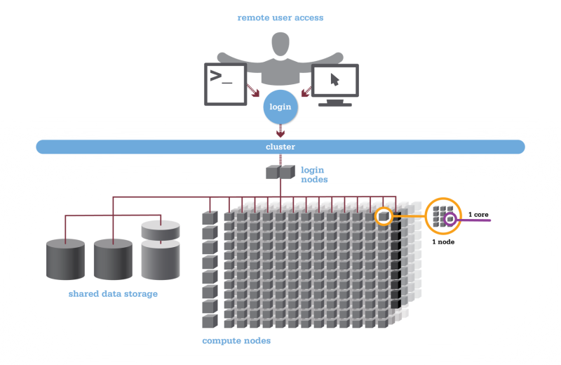
So here are three general points that it's good to keep in mind about what's the difference between your laptop or desktop and a supercomputer. So one way to think about a supercomputer is thinking about you know thousands or tens of thousands of individual computers that are linked together through a high, a very high-speed network, and so that you know, so you can, you know, link them all together so they can work together to do larger scale computing. That's really how we get the supercomputers. Another thing to keep in mind is that nobody is going to the computer itself. No one is standing in front of the supercomputer and working with it directly through a you know, a monitor and a keyboard. Everybody is remotely connecting to these systems. So they're all you know in in a in a separate, a separate area, you know, and we're all logging into them remotely. And so it's just important to keep in mind that your activity on the system is kind of moderated by the network that you're using. So if you're on a fast network, you know, you're going to get really good integration with what you're doing and really good response rates. If you're on a slower network, if you're, you know, somewhere with a slow wi-fi connection, you're going to see a slower response. So just keep that in mind when you're working with the systems. And then the third point is that these systems are shared. So you saw that, I said we have over almost 8,500 clients active on our systems this past year, and so at any given time hundreds of people are logged on and using the system or running jobs. So there's just some things that we ask you to do, so that we can all use the system, and everyone can have their jobs completed and their research move forward as efficiently as possible. So there's certain things that that the system we have, the system set up in a certain way, so that it can be shared effectively.
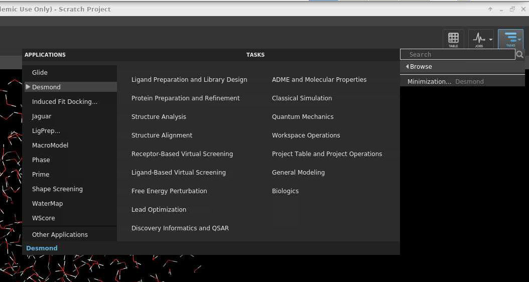
[Slide: “HPC Terminology”]
So here's some terminology that's good to know for using HPC systems. So we talk a lot about a node or a compute node. And so a node is sort of the unit of a cluster, and it's it's kind of equivalent to a high end desktop. It has its own memory, it has its own storage, it has its own processors. And so you know, each of those nodes is sort of like a desktop computer, and then they're all linked together, and they create the cluster. And so the compute cluster is that group of nodes that are connected by a high-speed network, and that forms the supercomputer. So, a supercomputer and a cluster, or a about synonymous. And a core we often talk about a core that usually is, relates to a processor or a CPU, and so you'll see I'll explain our hardware in a minute, and I’ll talk about cores per node. So that's really processors CPUs per node. And so, there's usually multiple cores per processor, chip and per node. And so you need to know that architecture when you make a request to the system. And then, finally, we refer a lot to GPUs, and those are graphical processing units. So, this is a separate type of processor that does much more kind of very parallel work. We refer to it often as an accelerator because it it's really good at doing some, you know, a lot of small calculations really, quickly, and so depending on the type of work you have to do, if it can be broken up effectively to use a GPU, it can speed up your work a lot. So GPUs have become very popular in lots of different workflows. So they're a big part of super computers now.
[Slide: “Memory”]
And some of the things to keep in mind memory is the really fast storage that holds the data that is being calculated on. So in an active an active job or simulation or analysis, memory is holding the data that's being used for that analysis. And so in a supercomputer we have memory, that is, you can have shared memory, some memory that's shared across all of your processors on a single node. The memory will be shared for all the processors on that node. If you use more than one node in your calculations then you're going to have distributed memory where the know the memory on one node won't be the same as the memory on the on another node, and you have to make sure that your calculation has all the information it needs. So, there's different types of decisions you have to make about how to use the system to, you know, speed up your code as much as much as possible, taking into account the different memory that's available to you. And each core has an associated amount of memory. So, we don't require that you tell us how much memory you need you just make a node and core request, and then we give you a relative amount of memory associated with that number, of course. But I'll go into more detail with the hardware.
[Slide: “Storage”]
And for storage. So, storage is where you're, you're keeping things for a longer term. Then you would keep you keep data in memory. And so you can have storage that is, you know, active in a in an active job holding, you know, data that's already been created, or it's already been analyzed. And you just need that for your output. And then there's longer term storage, for you know different purposes as well, and I’ll go over our data storage options at OSC.
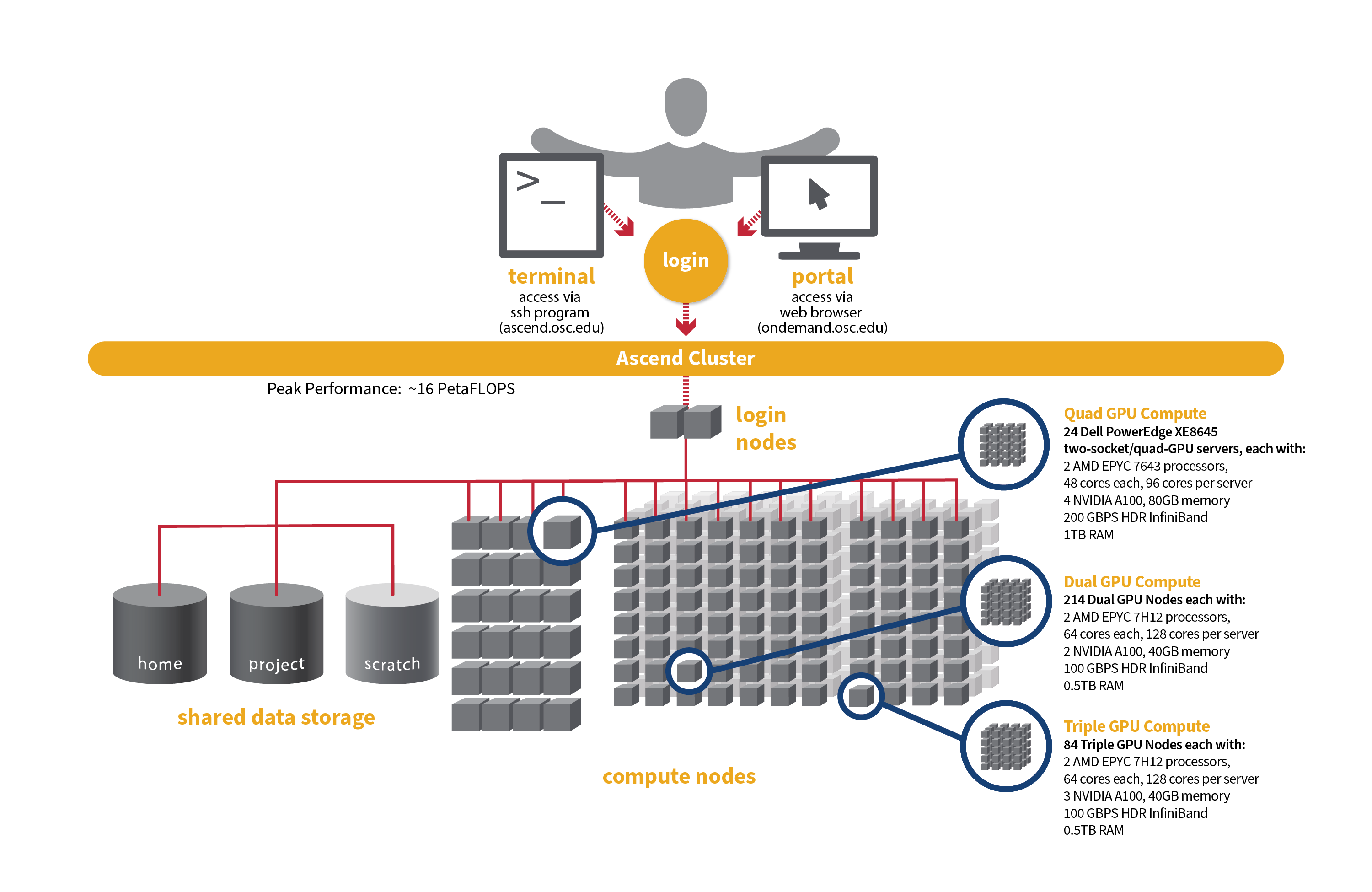
[Slide: “Structure of a Supercomputer”]
And so here is just a way to look at the supercomputer kind of covering all these concepts. So you can see the compute nodes are labeled at the bottom, and so those are the individual nodes that are network together to form the cluster. So that's the main part of the supercomputer. We have a separate type of node called the login node. That's for just kind of setting up jobs and reviewing output, but not for your main compute. And then you, as the researcher, are accessing this through some kind of network, either using a terminal program or a web portal. And then every and then the data storage options are available, you know, to access through the login nodes and the compute nodes as well.
[Slide: “Hardware Overview”]
So, any questions about general HPC things or General OSC surfaces. So, I'll go on to talk about the hardware that we have at OSC.
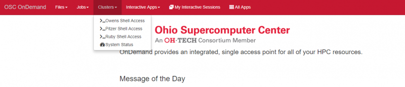
[Slide: “System Status”]
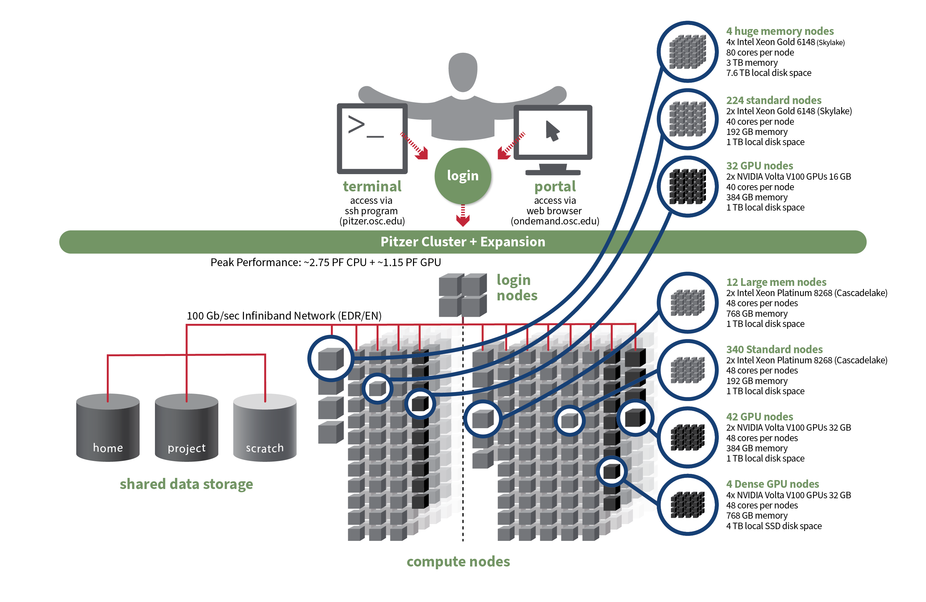
So at this point, so right now we have three systems that are currently active, and that's Owens, Pitzer and Ascend, and Pitzer is really divided into two sections. The original Pitzer and Pitzer expansion. So that's what you see here. So, Owens has been around the longest, Ascend just came online at the end of last year. And so, the larger systems are Owens and Pitzer. You can see if you look at the node, count that Ascend is a lot smaller. It's more specialized. So, it's a GPU focused system. So, unless you have work that is really GPU heavy that you need, GPUs, you may not, and you may not Ascend at all. Owens and Pitzer are still our main systems. And then, so yeah, that kind of gives you the general sense of the systems. But now I’m going to talk more specifically about each of them.
[Slide: “Owens Compute Nodes”]
So on Owens, Owens has 648 standard nodes. Those are standard compute nodes, and each of those has 28 cores or processors per node, and 128 GB of memory. So that's a standard compute node on Owens
[Slide: “Owens Data Analytics Nodes”]
Owens also has 16 large memory nodes. Each of those nodes has 48 cores per node and one and a half terabytes of memory, as well as 12 TB of local disk, space or storage. And so those are, for you know the types of jobs that need just a lot of memory to, you know hold all the data that's being, you know, calculated, or to do all the analytics that needs to be done.
[Slide: “Owens GPU Nodes”]
And Owens also, in addition to the regular compute nodes, has a 160 GPU nodes. And so, these are the same as the standard compute nodes so 28 cores per node, but they also have one NVIDIA P100 GPUs on them. So, each node has one GPU.
[Slide: “Owens Cluster Specifications”]
And so here is kind of all those parts of Owens put together. And this may be hard to read. It's not very large. But you can definitely look at all of these details and more specifications on Owens on our main website. If you just go under cluster computing, and you can choose Owens. You can see all these details.
[Slide: “Pitzer Cluster Specifications Original”]
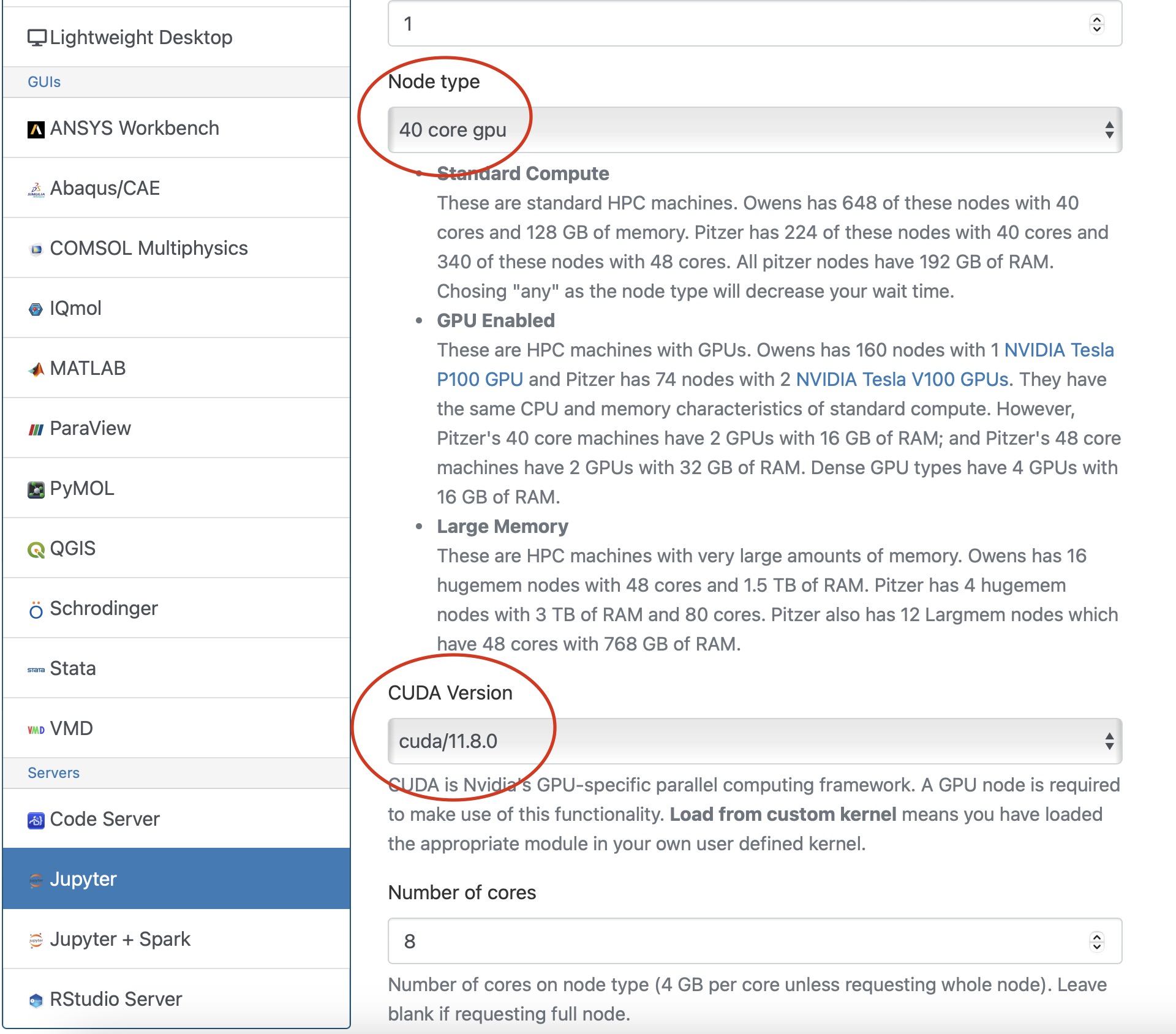
And so here is the overview for Pitzer. So this is the original part of Pitzer. And so this has 224 standard nodes, with 40 cores per node. And 192 GB of memory, and a terabyte of local storage per node. There's also 32 GPU nodes on Pitzer with the same 40 cores per node.
There's more memory, and there's two GPUs per node on Pitzer. So it's depending on the workload you need to you need to run. You might need, you know, two GPUs per note instead of one. And then there are four huge memory notes on Pitzer as well. Those are 80 cores per node and 3 TB of memory. So again, you know, these are for jobs that need a lot of single node parallelization. So you can use a lot of cores on one node, and you need a lot of memory.
[Slide: “Pitzer Cluster Specifications”]
Here we go, and so Pitzer, so the expansion of Pitzer, in addition to the original Pitzer, the expansion has 340 standard nodes, and those each have 48 cores per node. And then 42 GPU nodes as well. And again, those are two GPUs per node. And there's also 12 large memory nodes on the Pitzer expansion as well. And for dense GPU nodes so for jobs that that can take advantage of, for you can use four GPUs per node we have a couple of nodes for that as well. And again, the details of this are on our website. That's where you can see all of the technical specifications for our clusters.
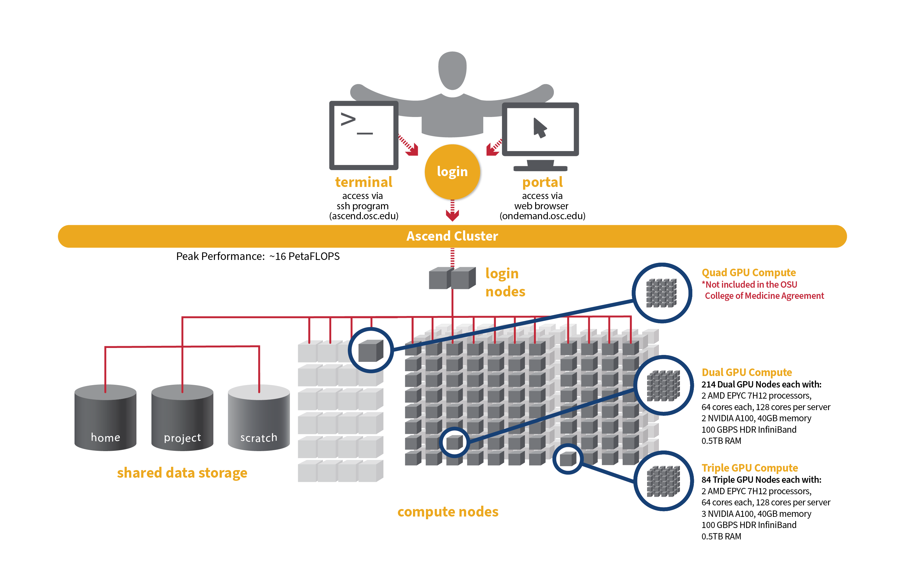
[Slide: “Ascend Cluster Specifications”]
And so Ascend like I said, it's the newest system. It's much smaller in in sort of node counts than Owens or Pitzer and so it's mainly focused on GPU nodes. So Ascend has 24 GPU nodes, with 88 total cores per node and 4 GPUs per node as well. So yeah, like, I said, this is GPU focused system. So, if your if your work is going to be, you know, very GPU heavy you can request access to the system, but we didn't give general access to everyone because it's not very large, and it's kind of specialized.
[Slide: “Login Nodes - Usage”]
And just to reiterate the login nodes. So, each of the systems has login nodes, and so that's when you first log into the system you're on the login nodes. And so, this is where you will set up your files, edit files, you know, get your input data and everything together to submit a job to the batch system so that you can access the compute nodes. This is not where you're going to run your jobs. There's very small limits on the login nodes as to how long any process can run, so if you start a process of some kind, it'll get stopped after 20 min. And you only have access to 1 GB of memory on the login nodes. So, they're really not for compute that you can do some small scale work, you know, like opening a graphical interface, or compiling like a very small code as long as it's really, you know not very compute intensive and won't take very long. But you don't want to use it too much, because it can slow down the login notes for everybody else. So the login nodes are mainly for setting up your jobs and looking at output, not for actually computing. And that's why we want you to use the batch system to use the compute nodes.
[Slide: “Data Storage Systems”]
So now I’m going to talk about our data storage systems. Any questions?
[Slide: “File Systems at OSC”]
So we have several file systems that OSC for different purposes. I'm going to talk about four of them. So, you can see them here on the data storage on the left. We have the home file system, the project file system, the scratch file system, and then the compute nodes. So, the storage that's available on the compute nodes. Those are the ones that I’m going to focus on.
[Slide: “Research Data Storage”]
And so the some of the features of these different file systems, the home location. So every account, so if you have an account at OSC, you'll have a location that that's your home directory, and that'll be on the home file system. And most accounts will have 500 GB storage available in the home directory. There might be some accounts that that have less, but almost all of them will have the 500 GB, and this is the main place that we expect that you can use to store your files, and we back this up regularly. So if you happen to lose something, or accidentally delete something vital, you can let us know, and we can help you restore it. So, we consider this kind of permanent protected storage. And then but if your group or your project needs more storage, then is available in each of the user accounts, then the project PI can request access to the project file system. And so this is just like a supplemental storage to the home directories. Most PIs or most groups need about one to 5 TB of storage on the project file system, and it's accessible to everybody in that project. And then there's also the scratch file system available. And this is available to everyone, you don't have to request access, so you can access it directly, and this is, we consider temporary storage. So we don't back up the scratch file system so you can use it, for you know large files that you might not want to fill your home directory up with. You can put them there if you're going to be actively using them, for you know, a couple of weeks or months, and you just want to keep them, you know, somewhere else than your Home Directory. That's what the scratch file system is for. And then on the compute nodes each compute node that you'll have access to will have its own storage. And so it's for use during your job. And so ideally, all of your compute. And you know, file creation, file, generation output, creation will happen on the compute node, and then at the end of the job you'll just copy everything back to your home directory. So you're not, you know, using the network to during your job to read and write. It just makes your job more efficient kind of reduces the overhead of that of that network usage, but you only have access to it while your job is running. So at the end of the job, you all that information is removed. So you said to make sure to copy back your results at the end of your job. We also have archive storage. So if you have some data set or database that you want to have, you know, stored for a longer period of time. They're not going to access regularly. You can talk to us. You can email OSC help and ask about that as well.
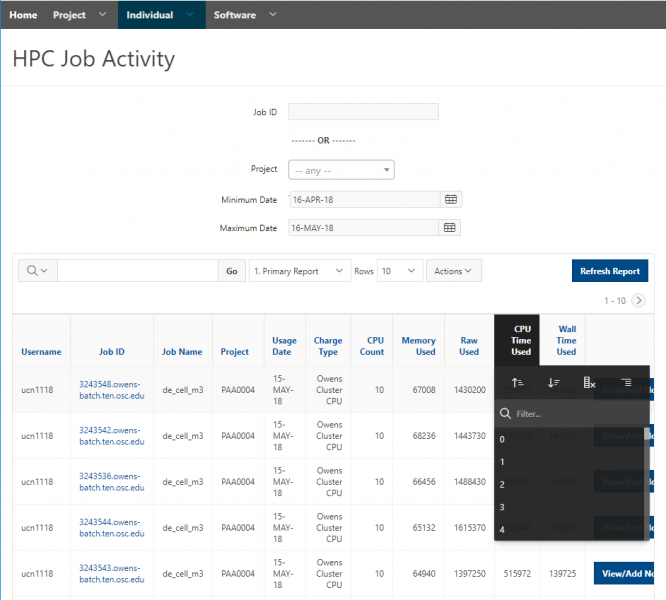
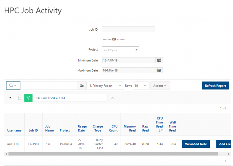
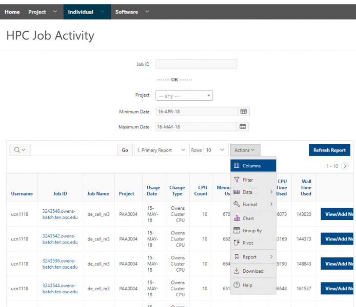
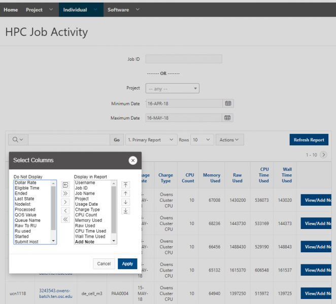
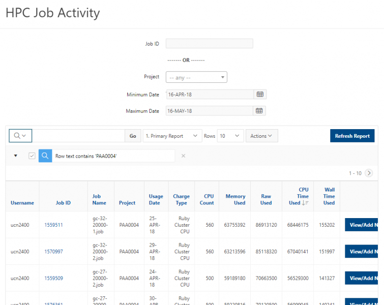
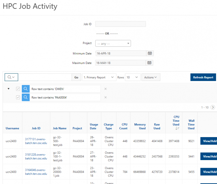
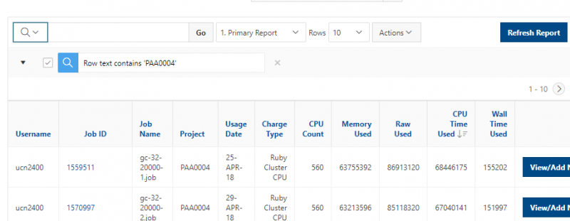
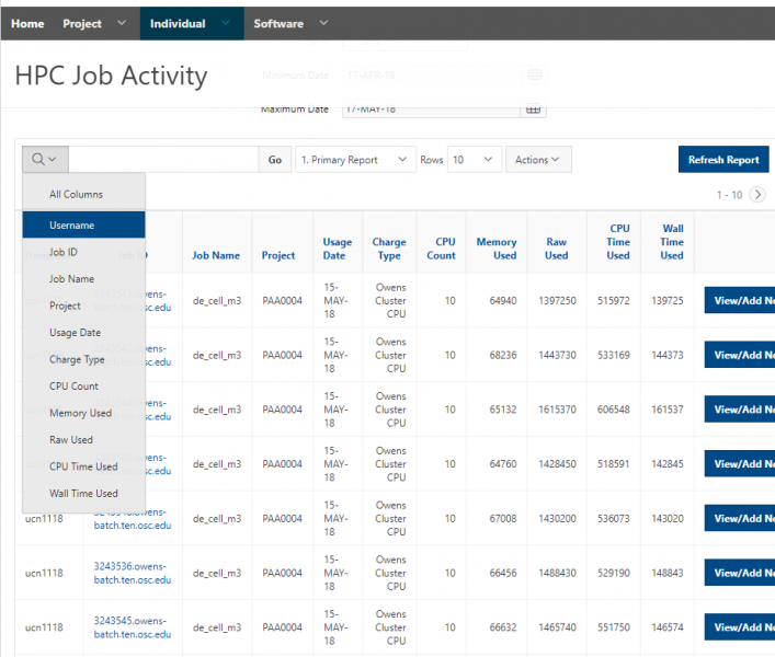
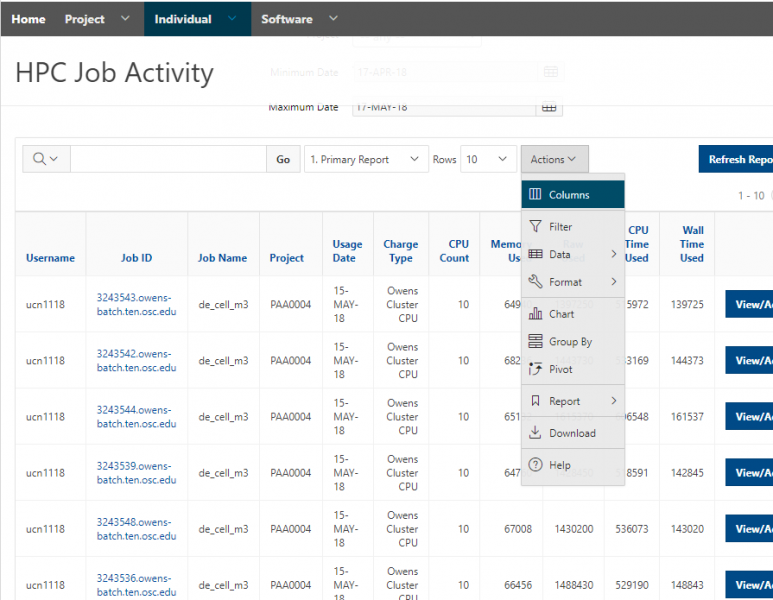
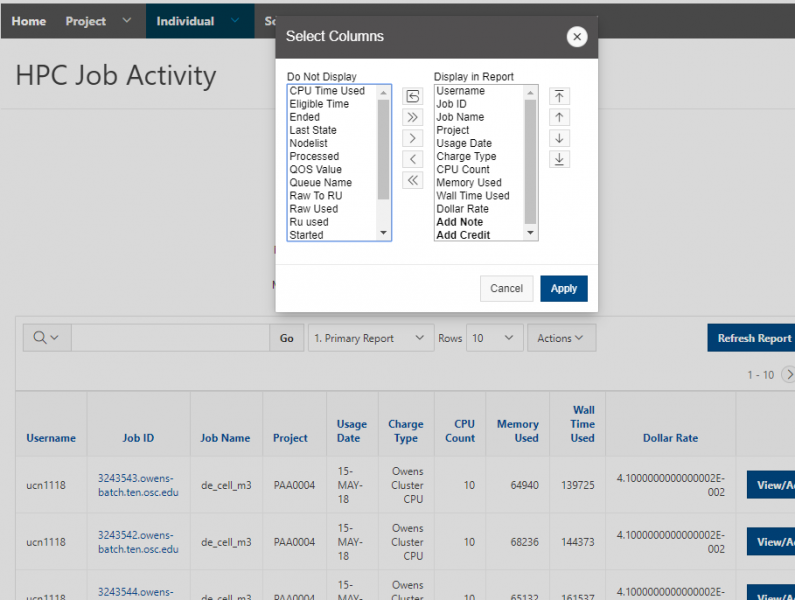
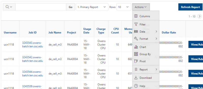
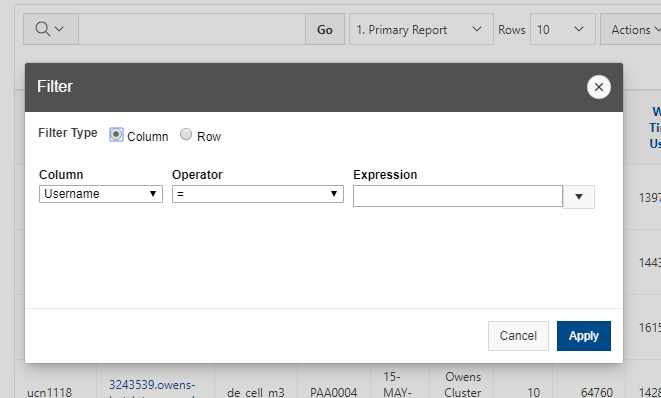
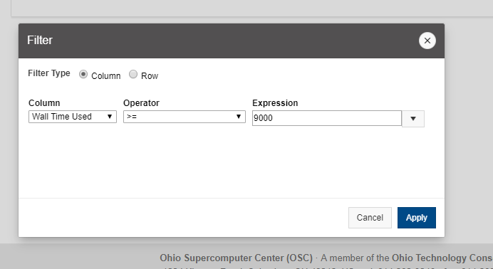
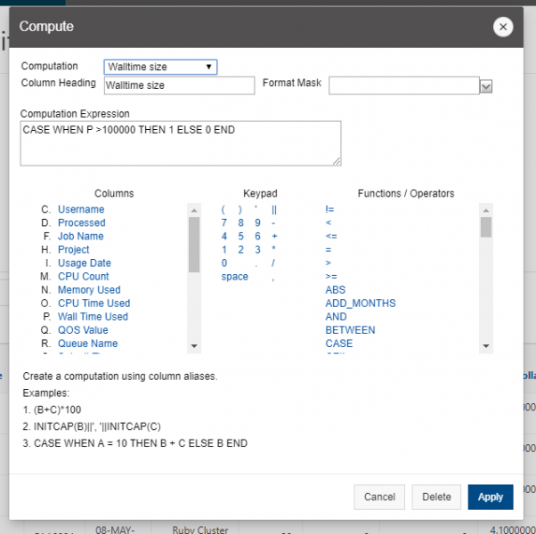
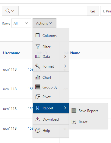
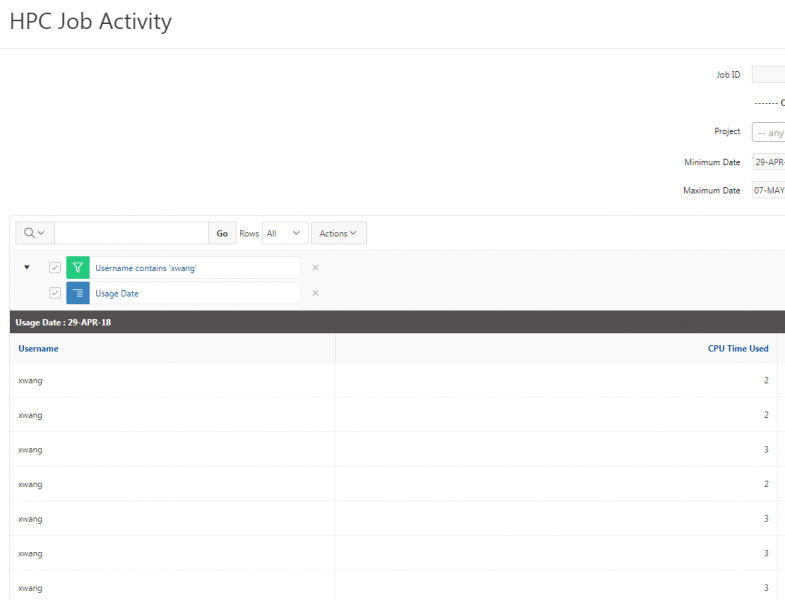
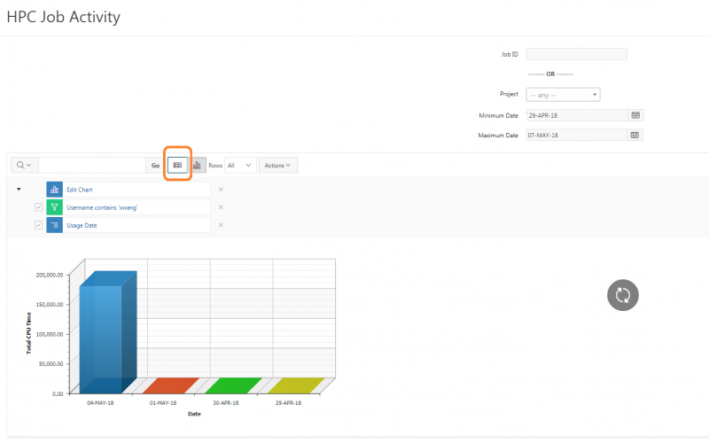
[Screen: Table showing Filesystem, Quota, Network, Backed-Up?, Purged]
And so here's just kind of an overview of the different features of the file systems. So, and I've included on the on the left. So the name of the file, the file system is home. You can use the variable dollar sign home as a reference to your home directory for the project file system. It's FSESS or FS Project, I think it's just FSESS. And then your project code to reach your project files. If you have that as a separate request the scratch file system you can reach by FS scratch, and then your project code, and then you can reference the location of the compute. Compute node storage with the TMPDIR and you can see the quotas so generally the quota for the home directory is a half terabyte. The project file system is you know amount that you choose. That's by request. We have a nominal quota of a 100 TB on the scratch file system and the compute. The compute file system varies, but it's usually at least 1 TB per node. You can see the different network speeds for the file system. So like I said, the home and the project or not very fast, the scratch file system has a faster network. So that is, you know, if you wanted to keep a large data set on the scratch file system and use it during a job. The scratch file system is more optimized for that. The home and project are backed up, scratch and compute are not. And we do have a purge on the scratch file system about every 90 days, so that is, if you have some files out there that you haven't used in a while, you know if they're you know. If they get old, they haven’t been they haven't been access for 90 days, they might be purged. We don't always purge, but when it gets full, we do, and then the compute node file system is removed when your job ends, so you only have access to it while your job is running. And again, there's links here on the bottom about where you can get more details about the file systems.
[Slide: “Getting Started at OSC”]
And I see information question in the chat. But sounds like you got the information you needed. So any other question, any questions about file systems or hardware?
Olamide E Opadokun:
Yeah. So the other file types that are backed up, for how long are they kept on the system?
Kate Cahill:
So you mean, like in the Home Directory?
Olamide E Opadokun:
Yeah.
Kate Cahill:
So there's a couple of layers to that. So Wilbur, do you know what our current scheme is for that? I know we back it up like multiple times a day, but then we have offsite backups as well. So I think it might be up to two weeks, or maybe further.
Wilbur Ouma:
Yeah, I don't have the correct, all the information on that. Yeah. But I know we do back up almost several times per day. Yeah, but we've had some requests people coming back that maybe they inadvertently deleted some files or data, maybe the last, you know a month or several weeks, and we've been able to recover those.
Kate Cahill:
Yeah, so I would certainly say that if you, if you do find that something has been deleted that you want recovered to let us know as soon as possible, because, you know, we don't keep them, you know, for months back, or anything. So you don't want it to wait too long. But at least couple of weeks, I believe.
Olamide E Opadokun:
Okay. So they kept on the system for a couple of weeks and then deleted?
Kate Cahill:
So the backups. So it's, you know we take. We take backups of the home directories, and we can restore things that have been deleted from a from an earlier version. And then we have offsite backups as well. So if we, if we happen to have some problem with our system and we lose power, we have versions that are stored off site as well. It's just a question of kind of like, how long those like you how far back those backups go. But yeah, so it's more about, you know. If you if you remove something and then you want it back, we can restore an earlier version of it. Once you let us know that you need it again. But on the home directory and the project directory we don't remove anything, so it's entirely up to you what's on those.
Olamide E Opadokun:
Oh, okay, so that that's not what subjected to the long-term storage, the archive storage, because that's just always going to be available right?
Kate Cahill:
Yeah. So the archive storage is a separate storage. So it's not like we automatically archive your home directory. That would be, you’d have to ask us to put something on the archive storage. It would be separate.
Olamide E Opadokun:
Okay, thank you.
Michael Broe:
So the issue, I often I advise graduate students who are working with PIs, who have. So the PI has the OSC account, and then they move away. They go to different jobs that if they go. And so then they ask me, can I get access to my data again? And I'm just would like to clarify if the PI doesn't keep this under control. How long will the data hang around, or how can they access it. If and so they've moved on from the OSU. And so, they no longer have an OSU account and they're trying to get access to data from, maybe several years ago, because their papers just been published. I know it's a big issue, a difficult issue. But I just like to clarify what is going on there.
Kate Cahill:
Yeah. So when someone leaves OSU and is no longer active their account. So I mean, if like, if they're not, if they're not part of your group anymore, and you're not working with them. And you don't, you know you're not going to have them on your OSC account. You know their OSC account will kind of just sort of age. It doesn't get automatically removed, but it goes into a restricted state, and then it goes into an archive state, and we remove that home directory. So it's always a good idea when somebody is leaving, so like, you know, for the PI to make a backup of that of that students' information at OSC so they have access to it if they need something from an earlier project. But yeah, certainly, after a couple of years, and I don't think that we could, that we would still have the student’s home directory data available unless there was some, you know, archive process that we actually said, “Put this on an archive.” I think from our perspective it's up to the PI, the person that runs the project to, you know, make a backup of that information. So, they have it like, make it back up way from OSC.
Michael Broe:
Yeah, or the if they believe the project is going to continue it, it's on the project. It's going to be backed up in, as long as the project exists.
Kate Cahill:
Right, so, if so, yeah, if the student has data in their home directory that everybody else wants to have access to for the project to continue, they should move it to the project directory. That's the shared space between all of the accounts that will stay as long as long as the OSC, the overall project is still there. So, if you have that project that shared project space for everybody in your in your group. You can, you can use that as another way to keep that that information available to everybody else. But yeah, it's definitely something that has to be kind of, there has to be a procedure when somebody leaves to make sure that that data isn't lost.
Michael Broe:
Yes, great, that's the perfect answer. Thank you.
Kate Cahill:
Alright great, so I’m going to start to talk about how to get started at OSC. So, this is more about getting an account and getting a project, and how we manage those things here.
[Slide: “Who can get an OSC Project?”]
So we have different types of projects that are available. So our main type of project is the academic project. And so that's generally led by a PI, and that person is generally a full-time faculty, member or research scientist at an Ohio academic institution. They could also. That's the main type of PI that we have at OSC for academic projects. And so the PI can request a project, and once they have that project, they can put anybody on it that they want, so they can authorize accounts for, you know, students post docs, other faculty, other their staff collectors, people from out of state people from out of the country. Anybody can have an account. But the PI has to have a certain role at an Ohio institution. Another type of project that we have is the classroom project, and so those are for specific courses. So, they're shorter-term projects that are kind of you know, specialized for giving students in a class access to OSC. We also have commercial projects available as well, so commercial organizations can purchase time at OSC as well.
[Slide: “Accounts and Projects at OSC”]
So a project we define a project code. So when you request a new project we'll define a code it becomes with a P, usually has three letters and four numbers, and that is like, I said, headed by a PI and includes any number of other users that the PI authorizes. And this is, and the project is the is how we account for computing resources. An account is a specific user so that will have a specific username and password. And that's how that that person will access OSC systems and the HPC systems. And so, an account is one person. So every person should have a unique account. You can work on more than one project, but you'll just have the one account to access all of them.
[Slide: “Usage Charges”]
And so we do charge for usage of our systems, and those charges are in terms of core hours, GPU hours, and terabyte months. And so, a project will have a dollar balance and any services that you use like compute and storage are charged to that balance and you know we are still subsidized by the state, so our charges are still partially subsidized, and so they're cheaper than your, you know commercial cloud resources. You can see more details on the link here. And yeah. So, if you're interested in in sort of the charges, the specific charges.
[Slide: “Ohio Academic Projects”]
So for academic projects annually, each project can receive a $1,000 grant so that can be your budget for the year, and so that that rolls over every fiscal year. So it'll be the beginning of July. You know, all academic projects will be eligible for a new $1,000 grant and so that's a way to kind of, you know, have a starting budget, and you know, get to use OSC resources, fully subsidized. If you think you're going to need more than that, then you have to add money to that budget. And so we do it this way, so that there are no unexpected charges. So you don't have some, you know, jobs that are over running, you know, or you know that somebody submits too many jobs or they're too big, and they end up charging more. The budget is a hard limit, and we also don't do proposal submissions anymore. We used to have an Allocations Committee that would review proposals, but we don't have that now, since we have this this fee model. The classroom projects that I mentioned before are fully subsidized, so they will have a budget as well. But it is not a budget that will be charged to anyone. And all of these the projects and getting an account are all available at our client portal site which is my.osc.edu.
[Slide: “Client Portal- my.osc.edu”]
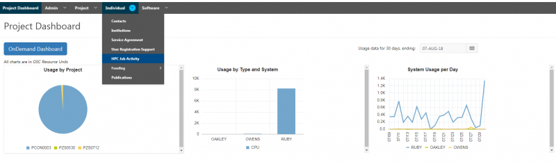
And so the client portal, like I said, is mainly for project, management and account management. It's really useful for PIs to kind of oversee the projects, the activity on their projects, so you can. When you log into the client portal. If you're on a project, you'll see some statement about the usage on your projects. So, you can see it broken down by project, by type and system, by usage per day, and then below you'll see your active projects, and then you'll see your budget balance and your usage. So, it's just a way to see that information at a glance, and then you can, you know using the client portal, you can create an account. Keep your email and your password updated. Recover access to your account, if it's restricted, change your shell if you don't want to use the standard batch shell you can change to a different shell, and then you can do things like, manage your users, and request services and resources like storage and software.
[Slide: “Statewide Users Group (SUG)”]
And so OSC, you know, has a statewide users group. So that's you know everybody that uses OSC to give you a chance to provide advice to OSC. So we can hear from the OSC community about. You know what they would like to see OSC do in future kind of where you want to see us go as far as resources or services. So this this group meets twice a year, and there's a chairperson elected yearly from the you know, Ohio Academic community generally, and we have some standing committees that meet as part of this group. So there's Software and Activities Committee and the Hardware and Operations Committee. And this is usually a day long sort of symposium that happens at OSC. But it's also a hybrid event where you can also share your research in poster sessions and Flash talks and meet other OSC researchers. And this happens twice a year, generally April and October. And you can check the OSC calendar to find out information about the next one, which is on April 20th. You can register, you know, present a poster send a flash talk, or just, you know, come and meet OSC staff and other researchers.
[Slide: “Communications & Citing OSC”]
So as far as communications we do send regular user emails, information about downtimes and any other unplanned maintenance events. We do have quarterly downtimes. We just had a downtime yesterday, so we're good for a quarter now. But we want to keep you updated. So make sure your email is is correct so you can receive those. And there's also information on our main website about citation. So if you are gone publish any work you've done with OSC resources, you can. You can cite the resource that you use
[Slide: “Short Break”]
All right, so we're going to take just like a five min break right here, so everybody can get up and move around a little bit, and we'll be back at 1:50. But does anybody have any questions? All right so I’ll be back in five minutes.
[Slide: “Short Break” beginning at about 41:35]
All right, so I’m going to get started again. Does anybody have any questions?
[Slide: “User Environment”]
So now we're going to talk about what it's like to use the systems and some information about HPC systems and software batch system environment.
[Slide: “Linux Operating System”]
So the user environment we use. We have a Linux operating system which is the most widely used in HPC so that's really common. If you have use HPC systems before you've probably interacted with the Linux system. It generally has been a command line based. So you need to have, you know some sense of the commands that you need to enter, to do things like, you know, refiles or move files. There is a choice of shells I mentioned. So bash is the default shell. But there are other shells available. If you you know, want to work at a different shell, you have to change your shell in the client portal. And so then you'll have that environment. And this is open-source software and there's a lot of tutorials available online. We have a couple linked here under the command-line fundamentals page on our website, just as suggestions potential tutorials. It's good to have some command line, comfort like. Just know a couple of standard commands to navigate the file system, for example. Just so you're comfortable in it, but you don't necessarily need to use the command line for most of your work anymore.
[Slide: “Connecting to an OSC Cluster”]
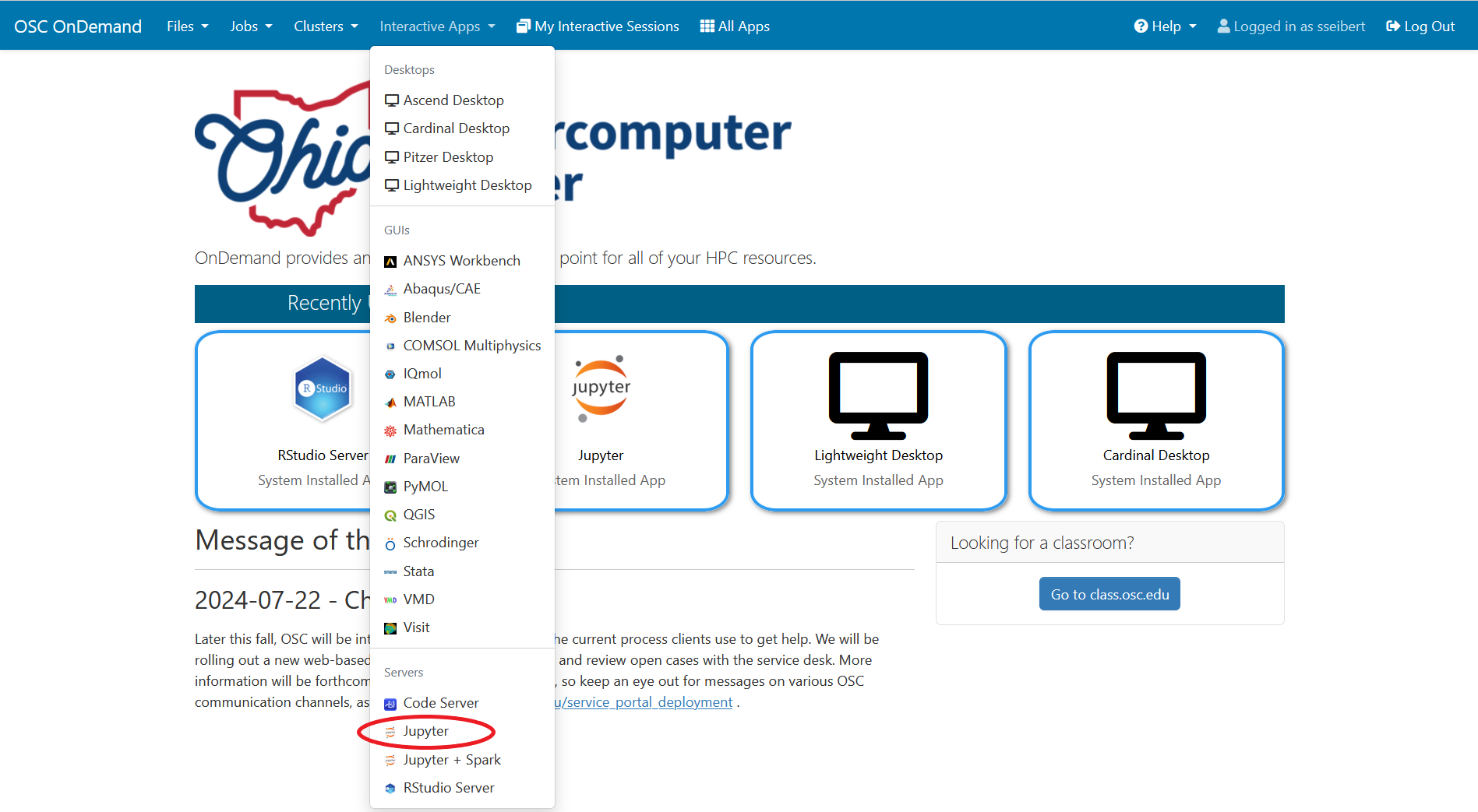
So to connect to an OSC cluster you have a couple of options like I said, everybody connects over a network. So you're going to use some kind of, you know. But you know, network connection tool. The historical way to connect to a system is using ssh through a terminal window. So in a Mac or Linux system you'd open the terminal program, and at the prompt enter ssh and then your user ID and @. And then the name of the sort of address of the system that you want to access. So you could access Owens it'd be owens.osc.edu and SSH. Is the command for secure shell. So you're connecting, you know, to the system through a secure shell. If you have a windows system, I believe there's a terminal program on there now, or you can download some free versions like putty is a terminal program you could use other options for connecting. So the main way that most of OSC clients, the connections, clusters these days is our on Demand portal. So that's our web portal. So you just need a you know you have a browser, and you just need to go to ondemand.osc.edu and enter your OSC user name and password, and then you have access to all the compute resources at OSC. Through the through the browser.
[Slide: “Transferring Files to and from the Cluster”]
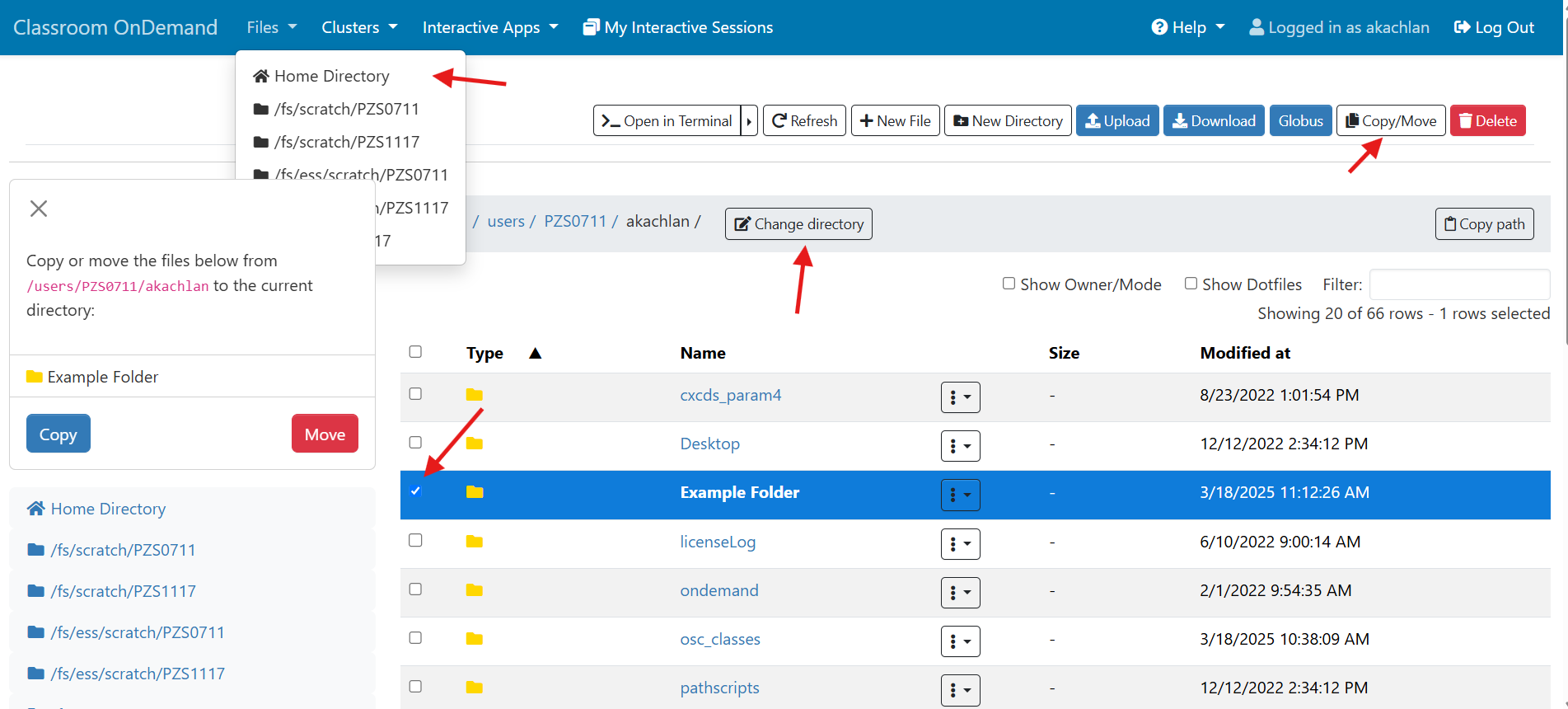
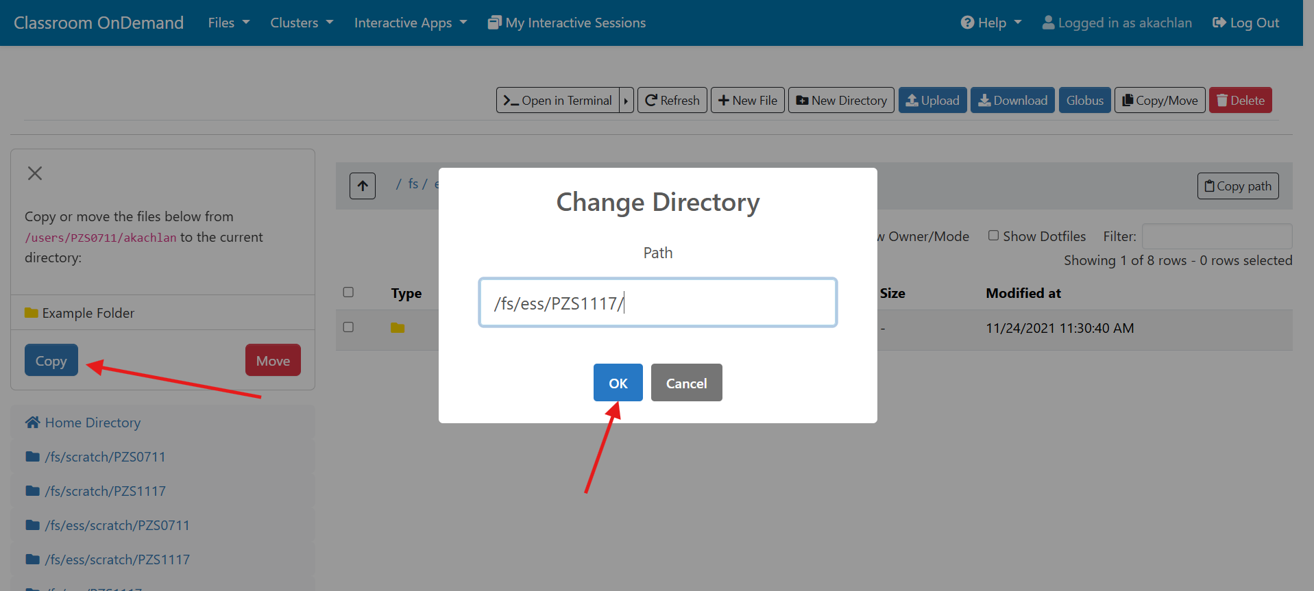
Another key step you generally have to take with transferring files. You know you have to take in your set up. Your research is to transfer files to and from the cluster. And so again, you have several options with the command Line tools. You can use sftp or scp, you know, in a terminal window. And so you would, you know. copy either from your local system to the cluster or the other way for smaller files. You can do that right through the login nodes so same kind of connection as the ssh, you can do owens.osc.edu. If your network is slow or your files are larger. You have another option called the file transfer server. So, instead of connecting to Owens or Pitzer directly, you would connect to sftp.osc.edu, and that just gives you access to the same file systems. But you're over a file transfer network that gives you a longer time to transfer file, so there's no time out on there. And so that helps with large files for slow networks. On the OnDemand portal. We have file management tools that include file transfer tools, so you can do a drag and drop to transfer files or use the upload and download buttons and the limit on that. It can be up to 10 GB. That's for very fast networks, so you can get, you know, fairly good size files to transfer again. It's network dependent. So you may see different outcomes depending on where you're connecting to the systems. We also have a tool called globus, and that is for large files or for large file trees. So if you want to transfer a bunch of structure, you know file structure all at once. Globus is another tool for that, and that is a web-based tool as well. It's a not an OSC tool it's a separate tool that we have an account with and you have to set it up once hyou have that it'll transfer files in the background for you and there's how to here Link on the bottom to show you how to get started using globus.
[Slide: “OSC OnDemand”]
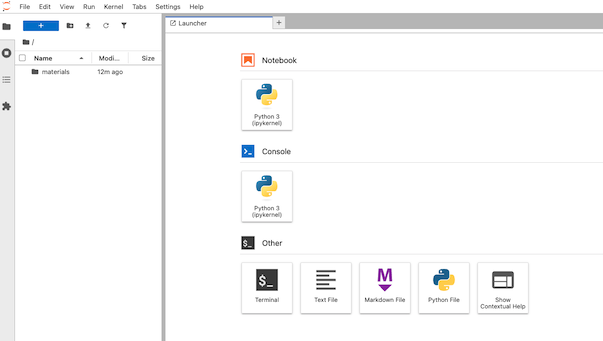
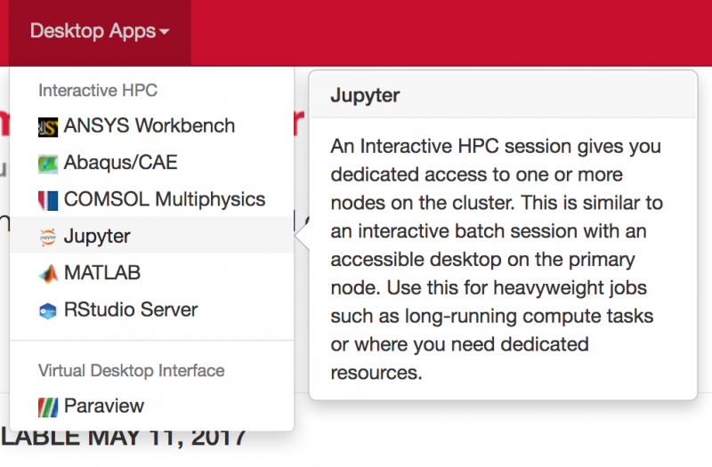
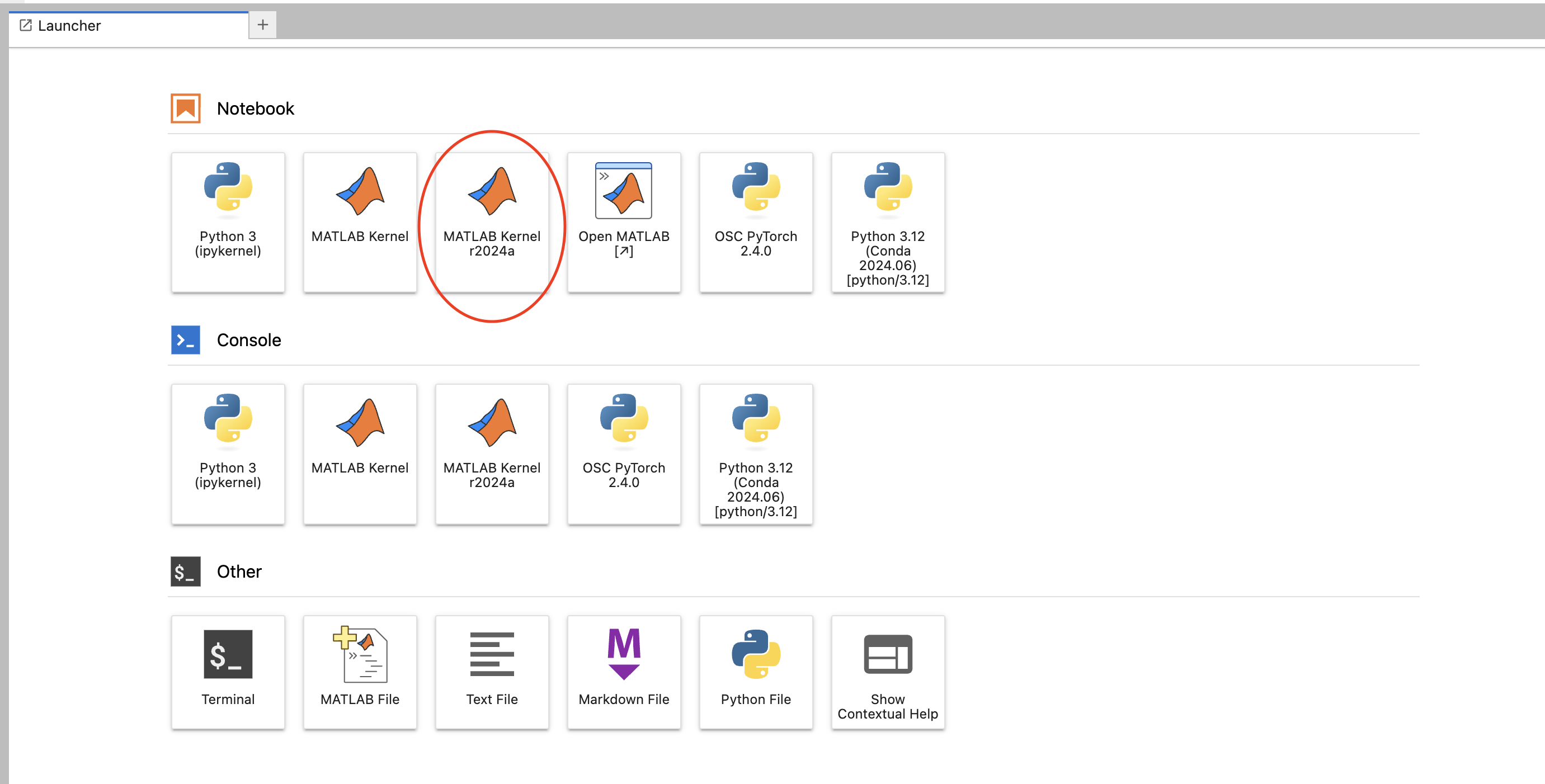
So I see a question. Can you access the HPC resources through a terminal? If you don't have an OSU account. So you don't have to have anything to. You know we we're not. We're not a high of state focus, so it's not OSU account. You do have to have an OSC account. So you have to have an account with us at OSC, and you have to have access, you have to have a project, you know that you're a part of that will give you access to the clusters, so you can go to our client Portal, which is my.osc.edu, and you know, get, you know, just create your own OSC account. But until you're on a project you're part of a project, or you've created a project that you're a part of. You won't have cluster access until then. So those are the things you need. And so here's some more details about our on demand portal. So like I said, it's ondemand.osc.edu and you can just open a browser window, and then you just need your OSC username and password to log in you can. You can do a kind of a connection, and then use a different credential. But you still need an OSC account, so you need to know an OSC username and password. And so, once you connect through the OnDemand portal you'll see tools like file management and job management, visualization tools and virtual desktop tools and interactive job apps for different types of things like MATLAB and R and Ansys, so it's pretty comprehensive. It's also a shell window, so you can open a shell and work at the command line as well.
[Slide: “Using and Running Software at OSC”]
So now I want to talk about using software at OSC. And how you get information about it, and how you get started working with it. So any question, any other questions about environment getting logged in? All right so software at OSC.
[Slide: “Software Maintained by OSC”]
Last time I checked which maybe out of date now we had over 235 software. Packages that we maintain at OSC for for our clients. And so there's a lot of lot of options out there. And so, if there's software that you're interested in, you can always so that the first thing you should do is check if we already have it on OSC. So you can check on our main site. You can look under resources and look at available software. And you can browse just a list of all the software or the list by, you know, by cluster or by software type. Or you can just do a search for the software package you're interested in. If we have it, if we support it, we'll have a software page on it, and the software page is really going to give you all the information you need about how you know what you need to know to use the software at OSC. So this will include version information, license information, and some usage examples. So it's really key for forgetting the information to get started.
[Slide: “Third party applications”]
We have, you know, the general programming software tools, various compilers. We have some parallel profilers and debuggers. So if you're writing your own code, you can use these tools to kind of optimize it, Ansys, we have MPI libraries, we have Java, Python, R. These are some of our most popular software packages. We also have parallel specific programming software. So the MPI libraries, OpenMP, CUDA, OpenCL and OpenACC for different types of parallelism for GPU computing and things like that.
[Slide: “Access to Licensed Software”]
So what software licensing is really complicated. But we try, when we support software at OSC to get statewide licenses for academic users as kind of our you know, base level of software access. And so we try and make that, you know, kind of the goal for all of our software, some software, even with that, as the license requires that individual people who are going to use it sign a license agreement. So check the software page it will tell you the details about what the license is, and if you have to take any steps because if you have to sign a license agreement, you can use the software until you've done that and we've added you to the software group. So check the software, page to get information about the license licensing, and if there's any requests you have to make of us. And also, like I said, the software page will have details about how to use the software. So some software also requires that you like put it into your batch script that you are like checking out a license. So you know, specifics like that, you'll see on the software page
[Slide: “OSC doesn’t have the software you need?”]
If we don't support the software that you need. So if you want to use software that that we don't have installed, and we don't maintain. If it's a commercial software package, you can make a request to OSC that you think it this should be included, because you think there's a group of researchers who would use it. So it's about kind of how important it would be to you know a certain number of researchers. We can consider it and add it if it if it seems reasonable. If it's open source, software you know something that you can download yourself. You can install it in your home directory. So that's something that that you can do, so that you and your group members can use that software and we have a how to on kind of the steps that you would take to install as to in software locally, and certainly the you know, whatever software you'd want to install would probably have details that you'd have to read up on to see, you know what the steps are for installing it. And then, if you have a license to, you know, for a commercial software that we support, or you know we can install. We can help you use that license at OSC as well. So there's several options for, software and we can definitely answer any questions about. You know software usage as you as you're trying things.
[Slide: “Loading Software Environment”]
So once you know the software that you want to use. We use software modules to manage the software environments so that we can maintain the software, you know, in a specific location, make updates, add new versions without you having to change all of your paths for the you know location of that software. You can just load the software module into your environment, and then you have access to all the software executables and libraries and things. So you need to use commands like module list. We'll give you the list of software modules that you have loaded already in your environment. So there are some default ones that everybody gets to begin with, and you can always change those. But we kind of have a standard environment that works for most people. So these are like these are command line tools. But you also are going to use these in in the batch scripts that you are going to create. So you should know these. If you want to search for modules, you can do module spider, and then a keyword or module avail. And then, when you want to add software to your environment, you do module load, and then the name of the software, and if there's multiple versions, you may have to be more specific about the version of the module that you want. And you can unload. You can remove things with the module unload, and you can swap versions of software with the module swap command.
[Slide: “Batch Processing”]
So now we can talk about batch processing. Now that we have kind of all the all the pieces.
[Slide: “Why do supercomputers use queuing?”]
So the batch system is the main way to access the compute nodes on the clusters. And so that's kind of the main, I mean part of the system. So you need to know about the batch system so that you can get access to that computing ability. And so supercomputers use queuing so that you can provide all the information to the scheduler and the resource manager, and say, “I need this much of the system. So I need five nodes for six hours, and you know, and here's all the information about my job.” And so the system can take that information, and you know, with everybody else's requests. You end up in a queue, and once the resources are available, then your job will get access to the compute resources, and then it can run all the commands that you've included and do your analysis, and then you get your output. And OSC uses Slurm for scheduler and resource manager. If you're familiar with those so that's the tool that you should become comfortable with.
[Slide: “Steps for Running a Job on the Compute Nodes”]
And that's what we'll see. I'll show you an example batch script using the Slurm commands. And so here's just the steps that you'll go through to run a job to access. The compute nodes. You're going to create a batch script. You're going to prepare and gather your input files in in your home directory or your project directory. But wherever you are with your batch script, that's where your input files will be. You'll submit the job to the to the scheduler. The job will be queued. Once the resources are available, your job will run, and then your results will be copied back into your home directory when your job finishes.
[Slide: “Specifying Resources in a Job Script”]
And so the resources that you have to specify in a job script. I've mentioned them, you know, a couple of times. You need to and specify a number of nodes number of cores per node. Request GPUs, if you want GPUs, you don't have to specify memory, so memory will be relative to the number of cores your request, so it's about 4 GB of memory per core. On the standard nodes. It's different on the on the large memory nodes. But there's still a relative amount. So you don't have to request memory while time is. How long you want to have access to those compute nodes. And so you want to have enough time for your job to complete, but not too much more than that, just because you're when you're requesting more resources than you need, and it will take longer for your job to start. So you do want to overestimate slightly. So you know, if your job is going to take 12 hours. You might want to request, you know, 14 or 16, just to make sure that your job is, you know, fully completed before the wall time ends. And this is something you get used to, you know. You just keep making requests and seeing how long your job really takes, and you get better at getting that wall time, you know. Request to be pretty close to your job needs. You include your project code. So that's how we account for usage. So we need to have that project code in there. And then if there are any software licenses that you have to request. You'll see on the software page. If the license, if the software you want to use has a license request, you have to include that'll be in your job script, too.
[Slide: “Sample Slurm Batch Script”]
And so here is what a sample batch script looks like. So the lines on the top are all are all directly, you know, information to the scheduler, so Slurm has to run in in the batch shell. So we put that bash call in there at the beginning and then all the S batch lines are lines to the schedule, or, you know, these are our specific comments that are directed at the scheduler. And so this includes the wall time. So this is a one hour request number of nodes is two, and n tasks per node is 40. So Slurm uses in tasks per node for cores. So this is two nodes, 40 cores. We give the job a name so that you can recognize it in the in the queue. The account is your project code. So Slurm calls project account, and so you put your project code there and then the rest of the job script are all the commands to run your job. So we just say, you know, make sure that we're starting in the in the directory where our job was submitted. Just so, because that's where our input files should be. So that that line CD Slurm: submit the IR that's just saying, make sure I’m in this directory and then we're going to set up the software environment. So we have a module load command. Then we're going to copy our input files over to the compute node. So the copies CP is copy, hello.c is our code, and we're copying it over to the compute node. And then we're going to so then we're going to run that. We're going to compile our code and then run that that job, get our results and then copy those results. The last line is a copy results, and then back to your working directory. So these are all the commands that we go into a batch script. And so this would be, you, you know, create this as a text file and give it a name and save it.
[Slide: “Submit & Manage Batch Jobs”]
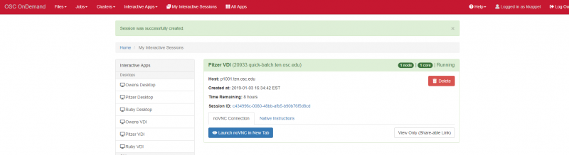
And so, once you have that ready and your input, files are ready. You're going to use this command on the top S batch, and then the name of that job script to submit. If it works and it submits correctly, then you'll see a response, and it's right here, submitted job response,
Slurm response, submitted batch job and you'll get a code. And that is your job ID and that's a way you can reference that job in to the queue. So if you find that you made a mistake in your job script or something, you want to cancel that job you do S cancel and then that job ID so this code here if you wanted to pause your job or hold it before it starts to wait for something else to finish you can use S control hold in the job ID, S control release job ID will release the job from hold. And then if you just want to look at the all the jobs you've submitted. You can do the SQ Command dash you, and then your user ID and that'll just show you what jobs you have in the queue at this point, and what their status is. You want to do that because that that the queue will be very, very long, and if you look at the whole thing, it won't really normally get much information out of it. So this is just kind of the very simple, simple information to get started submitting back jobs to a lot more information you could use to kind of make your jobs more complex or do more things with the batch system. We have several pages on our main website under batch processing at OSC. That have more details about all the different ways. You can use the batch jobs, and Wilbur teaches a training that is the batch system training to have more practice with the batch jobs so you can do some hands-on activities. And so that's another good option.
[Slide: “Scheduling Policies and Limits”]
And so we do have scheduling policies and limits for our systems. And so this is just so that you know jobs don't take over the whole system, or you know. So we have limits both on wall time. So we have for a single node job a wall time limit of 168 hours. For more than one to node jobs. We have a limit of 96 hour, and then we have per user and per group limits. So with number of concurrently running jobs is limited, and the number of processor cores is limited. So if you have many, you know so several large jobs you're limited in the total number of cores you can have in use. And so we have per user and per group. This is the, these are the current limits for Owens. They're not the same from system to system. So if you are curious, you can see those details in the cluster technical specification documents. You'll see a batch limit page that'll kind of give you these details, but you shouldn't unless you or your group are running many, many jobs you probably won't hit these limits.
[Slide: “Waiting for Your Job To Run”]
So how long it takes your job to run is based on how busy the system is, and what kind of resources you request. So if the system is really busy, it'll take longer for your job to start if you request resources that are more limited, like large memory nodes or GPUs, or particular software licenses that are popular. It'll just take longer for those resources to become available. And so I’ll show you on OnDemand how you can see what the system load looks like, so you can kind of if you, if you can, you know, choose which system to use. You can look at the system, load and see which one might start sooner.
[Slide: “Interactive Batch Jobs”]
You can also do batch jobs, interactive batch jobs, where you make a request. You get access to a compute node, and you use it. Live so you can do this from the command line. You can do this through OnDemand. And so this is useful for kind of small scale testing or you know, kind of work flow development, type activities where you want to kind of do things live and see how it goes before you, you know, submit a batch job that runs on its own. And so it's the same kind of you still have to use the batch system so you're still making a request to the resource manager and scheduler number of nodes, number, of course, wall time and then you get access to a compute. No, directly you want to, you know, keep in mind that a large request will take some time to start, and you have to be there when the job starts to use the compute node, because the wall time will start running as soon as the job begins. So this is a useful tool, and OnDemand a lot of interactive tools you can use with different software packages. But this isn't really where you should be doing most of your production work. This is more for testing and trying things out.
[Slide: “Batch Queues”]
Customers have separate batch systems. So if you submit a job to Pitzer, you can't see it in the queue for Owens. So just make sure that you know which system you're submitting to. We do have some debug, some debug reservations on our clusters as well. So if you run a very short job that you just want to test some part of your work. You can use the debug queue to run that quickly.
[Slide: “Parallel Computing”]
To use, you know the systems to get the most you know out of using the systems. You want to use multiple processors. You want to take advantage of the compute resources available. And so you know, that could be multiple cores and a single node. So you know, we have a lot of single notes that are 40 cores, 48 cores, that's a lot of processing just on a single node. That's a good place to start with parallelism to make sure that your job can take advantage of multiple cores and then you can, if you want, you can expand beyond a single core to multiple nodes. And you you're going to use, you know, different types of parallel tools for that to work. So, you have to learn more about MPI. And so, it depends on the type of work you're doing, you know, if you could take advantage of the different types of parallelism.
Michael Broe:
[Slide: “To Take Advantage of Parallel Computing”]
Can I just jump in here? Go ahead. This is Michael Broe. So use showed in a Slurm script before, like number of nodes. Let's say it's one, and then in tasks equals one.
[Slide: “Sample Slurm Batch Script”]
Yeah. Those two in tasks per node equals 50. But there's another Slum option which is CPUs per task. And I don't understand how that interact with tasks per node, and what your recommended procedure is with that.
Kate Cahill:
So I have not used that variation in Slurm. So CPUs per tasks, have you done that Wilbur?
Wilbur Ouma:
No, I haven't, but I have an idea of what it could be doing. So by default, Slurm doesn't equate the number of tasks to be same as the number of CPU cost that we using. So there's some pipeline in which you assign one task. So in Slurm the one tasks actually changes a lot. You could be doing, if you doing an MPI process, it could be the parent task, and then you have like the child tasks, you can have one parent Slurm task that it's running other child tasks that you can say, you know, that will be using different CPUs. So, to simplify things. What you've been like always see is to equate one Slurm task by default to be like one process right? But Slurm still comes with the option of specifying CPUs. Right so, and the reason is because Slurm differentiates CPU calls or processes from tasks like being one. But you just try to simplify that and make sure that okay to make it simple. You will put one processor or one process to be equivalent to one Slurm task. So for most of the analysis that that I do carry out. I don't need to specify the number of CPU, so the like the CPU option for Slurm. I just specify the number of tasks per node or number of tasks, if I'm requesting for one node. And that will by default translate to the number of process that I want for that particular analysis. Does that answer your question, Michael?
Michael Broe:
Yes, it does. I mean if I can ignore CPUs per task completely, I will. I just wanted to know if I was missing something. But if that's if it's a refinement, and it sounds like it's a very great refinement. It's not for this webinar, but it's good to know that what your default take on it is. So that's great. Thank you.
Kate Cahill:
[Slide: “To Take Advantage of Parallel Computing”]
And so yeah, when you're thinking about your parallelism. Make sure that the software you're using, or the code that you're writing is going to take advantage of multiple cores and or multiple nodes. So you want to make sure that that you know you have something that can run in parallel and that you learn about the parallel versions of software that you may already use. We have a tool called mpiexec. That's when you want to use multiple nodes and divide the work across them we use, for you know, so you can use the mpi tools it won't, miss, you know it's not necessarily going to work to just request more. No nodes or cores and it and your job will instantly run faster. You know, if you if it doesn't take advantage of those resources, it's not going to improve anything. So just keep that in mind and do some research on the tools you want to use, and how they work in parallel. So what information you need to know, to provide them so that they can work in parallel.
[Slide: “New – Online Training Available!”]
And so that is kind of everything I wanted to cover about the details about, you know, using OSC resources and then in a minute I'll switch over to a web browser and just show you OnDemand, so you can see what it looks like, but wanted to highlight a couple of things about how to get help and more information. We have some new online training resources available. So this is on ScarletCanvas. So we've got a version of ScarletCanvas from Ohio State. That is an OSC you know version of ScarletCanvas and so this is a free and available to everyone, not OSU, not Ohio State related and all you need to do is create a ScarletCanvas account, and then you can register. You can self register and go through these training courses. And so these are, you know, covers a lot of the material that I covered today, you know, in the OSC Intro, and then the batch system at OSC course we'll cover a lot of but Wilbur covers in his intro to OSC Batch. And so you can look, watch videos go through activities, do quizzes. Do some hands on, just to give you more practice, or a way to give you a reference for these services kind of get comfortable with some of the things, some of the concepts that we've talked about. And you can let us know if there's a certain, you know, certain type of training you'd like to see that we could develop for this as well. So we want to add some new things to this as we go and you can find that if you go to osc.edu, search for training. You get our training page, and you'll get the link for these courses.
[Slide: “Resources to get your questions answered”]
Other resources to get your questions answered. We have a getting started guide, so that I’ll just kind of give you information about different parts of the OSC resources that you can, you know, find information on our website. We have an FAQ that's useful to kind of check into before you, you know. Look for help elsewhere. See if see if that's already included in there. We have a lot of how to's. So these are sort of step by step, guides for doing different activities that people tend to need to do on OSC systems like installing software or installing R or Python packages or using Globus. So there's a lot of those. And then we do have office hours. So there every other Tuesday, and they're virtual so anybody can attend. We do ask you sign up in advance, so you can see them on our website on the event page. There's you know, an event for each one, but make sure you sign up in advance to reserve a time and then we do provide to some updates through the message of the day, which is when you log into our systems, you'll see a big statement, and that's the message of the day, and then we have a twitter feed called HPC notices, and that's just for system updates. So if you follow that you can get any updates we want to share about the systems.
[Slide: “Key OSC Website”]
And these are the main websites that I've talked about today. Our main page is OSC.EDU, our client Portal is MY.OSC.EDU and our web portal to access the clusters is ONDEMAND.OSC.EDU. And so any questions I’m going to switch over to the browser and open OnDemand.
[Switching to Browser]
But thank you for attending. If you, if you want to go before I start the demo go right ahead.
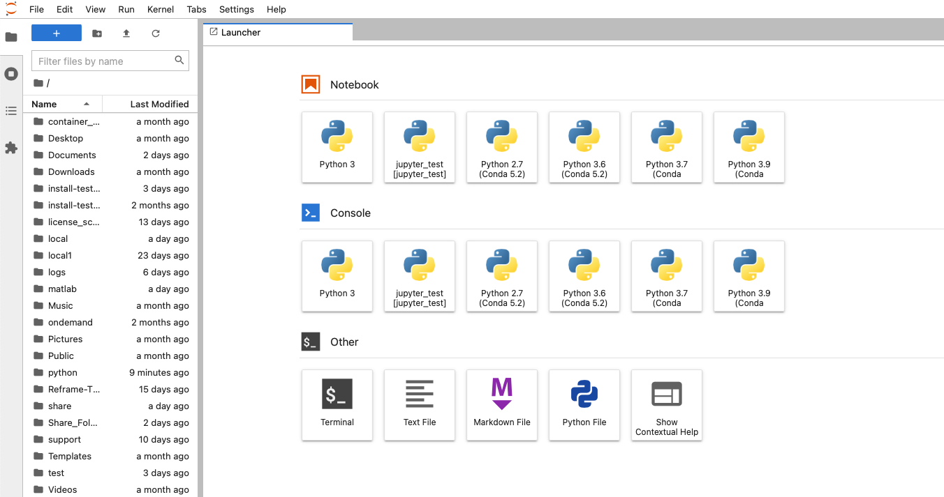
[ondemand.osc.edu browser]
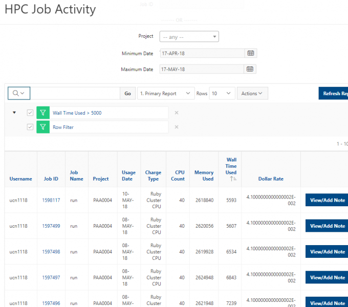
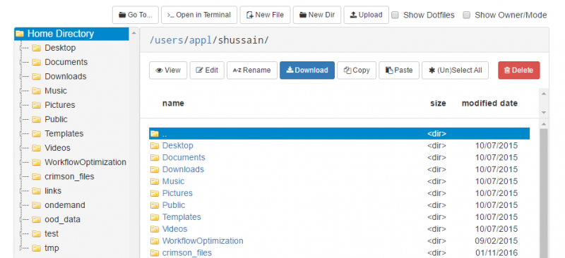
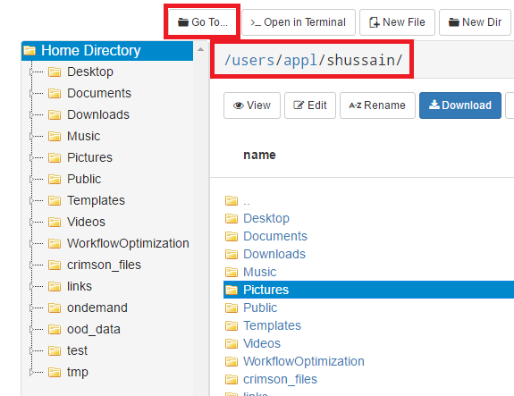
And so I was already logged in. But you just have to log in with your you with your OSC username and password. And then you reach the OnDemand dashboard, and you can see here, here's the message of the day and so you can see some information about, you know updates on Pitzer and general updates about classroom support. Over on the right, you can see we have a separate version of OnDemand that's specific for classroom projects, and that's class.osc.edu. So if you wanted to use OSC for a class you would, we could set up that environment for your class, so it'll so little more simplified and a little more targeted to classroom type users. But also you see some efficiency reports here. So we have some monitoring tools that we use that can tell you kind of how efficient your jobs are, so you can get a sense of sort of when you run a job. Are you using all the resources that you requested, or how efficient is your request? It's just a reference, just so. You kind of have an idea and then on the top here all the different menus for OnDemand. So we have our file manager. And so this will have the different locations that you have access to, so everybody will have a home directory. And then, if you have a scratch location for one, for a project that you'll see that or a project location and you can see the different project codes. So if you have multiple projects, you'll see different locations. If you click on any of your locations and you'll see this sort of file manager open up, and so then you can navigate into your folders. You can create directories or folders.
[Open OnDemand Browser showing File Page then File Example then File Page]
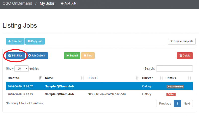
You can create files. You can upload and download and just manage your files. And you can also edit files here so pick one that might be good, so you can, you know, just view the contents of a file. You can edit a file so it can open it as a file editor and make changes to the file and then save them. And then, you know work with files, you know, through this. So you don't, you don't have to go to the command line. You can use this to manage and update and edit files. And so the jobs menu. This is where the job composer is a tool for submitting jobs. So it kind of helps you manage all the parts of creating a job like getting your input files together, creating a job, a job script. The active jobs are, that's just the queue. So once you submitted a job, you can look at jobs that are running. And so over. Here are some filter options, so you can look at your jobs, you can look at all jobs and you can focus on a particular cluster.
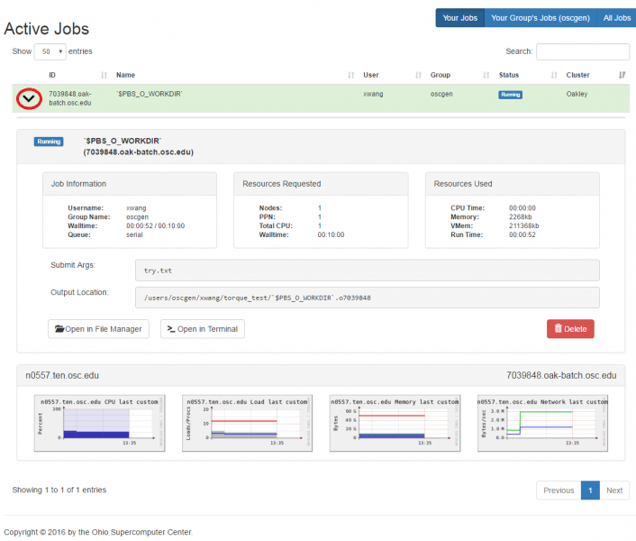
[Open OnDemand Browser Active Jobs Page]
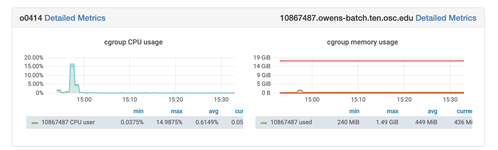
So if I look at all jobs on Owens, I can filter this, you know, so I have running jobs. I can look at. I can't spell. I can look at. You know jobs that are in a cued status. But one thing I wanted to show you is when your job is running, you'll be able to get some information about it while it's running. So if you click on the little arrow on the side. You'll get information about the job, so you'll see kind of the job ID. You'll see the requests this is one node 28 cores, the time limit, how long it's been running. But you also see these sort of detailed information about CPU and memory usage, so this can be useful to somebody trying out some new jobs to see, you know, if I make a request of a certain number of cores, is my job actually using all that resource. And so you can see this job is using, you know, about 20 of its CPU usage. And you know not much memory here, but you can get a sense of what your job is doing when it's using the resources. So that's a useful tool. Under the clusters menu, this is where you can open a shell window as a shell, you know terminal window, so you can, you know, use this to work in the command line. There's also a system status tool here, and this is what I mentioned.
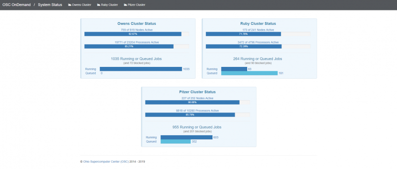
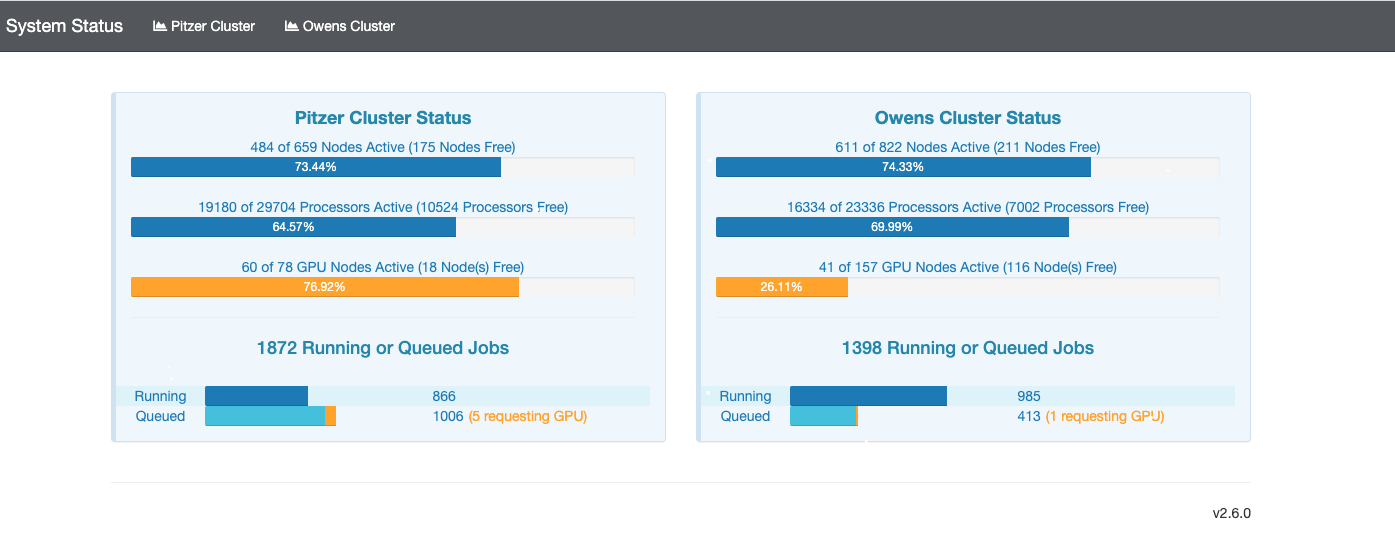
[Open OnDemand Browser Cluster Status Page]
If you were, you know, wanted to choose which system to use. The system status can kind of give you a sense of how busy the different clusters are, so that this one is Ascend. And so you may not, you may not have access to a send or may not need to use it, but you can see on Owens. It's about, you know, 70% full. And there's 164 jobs queued. Pitzer is partially offline right now, so even though it says it's not full. It's actually you know at full as far as what's available, so you can see that a lot more jobs are queued on Pitzer right now. So if you wanted to start a job now Owens might be a good option if you can use Owens.
[Open OnDemand Browser Active Jobs Page]
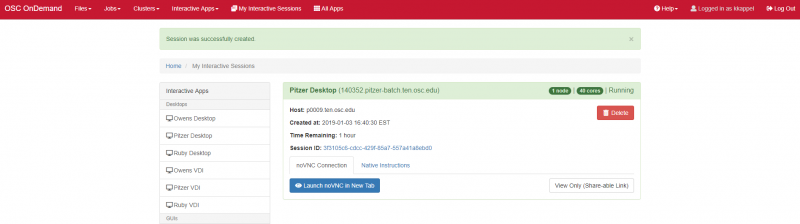
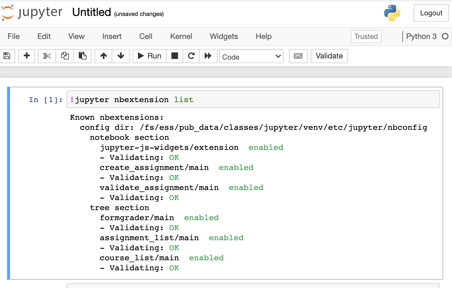
And so that's just the system status, and then the interactive apps are here. And so these are all tools that we've developed at OSC to use these different software packages for data analysis, visualization. You got Jupiter notebooks, Jupiter Lab, Jupiter with Spark and R studio.
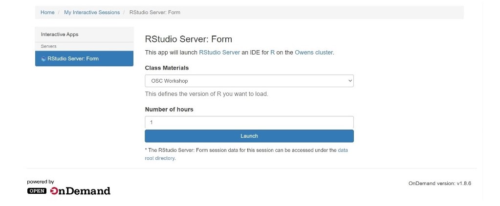
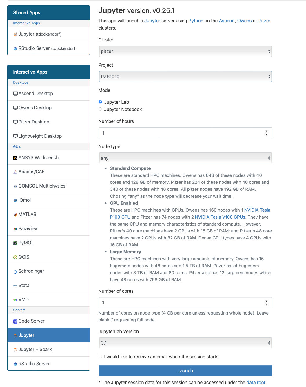
[Open OnDemand Browser RStudio Server]
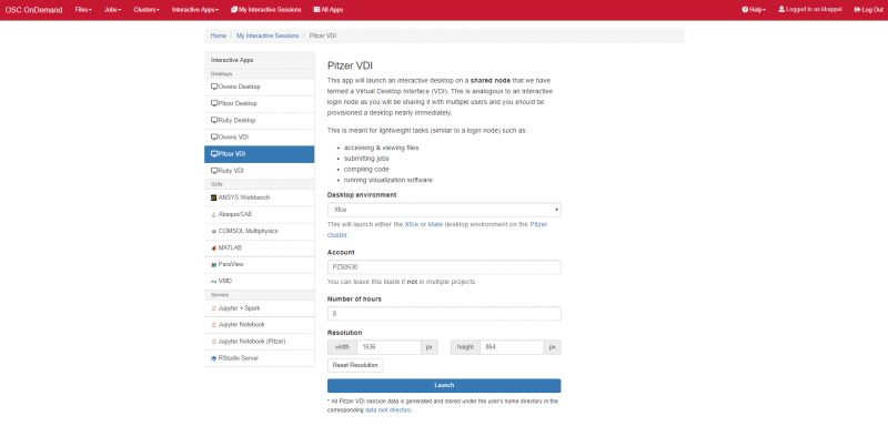
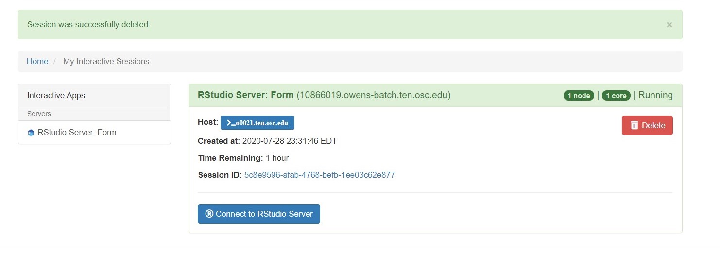
And so each of these are interactive jobs. So you're going to get access to a compute node. And so then you can, you know, use a tool that you may already be familiar with, to run on the compute nodes. Still, these are going to be fairly small scale, but it's a good way to get started. And so you just need to have information like what cluster you want to use, what version of our you want to work with. You have to put in your project code and you tell it how long you want your job to go, and then, if you want to use a specific node type, you can use a GPU node or a large memory node. But just remember, these are interactive job requests, so it's going to wait in the batch until these resources are ready. So if you, if you make a specialized request, it'll take longer, and then you can tell it number, of cores. And so when you launch this, it will once it once the job starts. So I've submitted this and so it's queued in the, you know it's waiting in the queue right now. And so once it starts I’ll open it, and it'll look like our studio, and I’ll have access to my files that are on the system, and I can, just, you know, run, run in R like I would if I was, you know, running on my laptop. But I’m using the compute resources at OSC. So this might take a while to start, because I choose Pitzer. Oh, it looks like it's starting. So it takes a minute to get started. And so now it's running, so I’ll click, connect to R studio and so that it'll just run R studio for me on Pitzer.
[Webpage running R studio via Pitzer]
And so then I, you know. So this is a good way to use the system to kind of get comfortable with running things. But again, this is not necessarily the best choice for production running. You still want to submit, you know, a job to run on the batch system kind of on its own. So you don't have to manage it directly.
[Previous Open OnDemand and R Studio Browser]
And so yeah, you can see other options over here. These are virtual desktops. So just another way to work in the system. You get a virtual Linux desktop, and then these are different graphical interfaces for different visualization and analysis tools. And Jupiter notebooks, like I said, is here. So that's really popular for classroom purposes. And that's those are the main features of OnDemand. So any questions?
Michael Broe:
Thank you very much. That's fantastic introduction. I have a question, but it's not a newbie question. It's about quarto and python. But if I can, you know, explain why you here? I will. But I don't want to get in the way of anything you want to finish up now.
Kate Cahill:
Sure. So I see a question. Do we have to be proficient in R to use OSC system or is the code generated automatically. So you do. I mean, if you want to use R you have to, you know, use some existing R code, or write your own. Wilbur is actually, you know, kind of one of our key R experts. But yeah, the code doesn't get generated automatically. You'd have to create some or use some existing code to do some to do some analysis with R. We do have some R tutorials in here as well. So, I don't know if you saw that when I was doing the interactive app. There is access to OSC tutorial workshop materials. And so that's just, it just gets copied into your home directory, and you can look at some R tutorial tools, so it's just example R code that you can work with. But it's pretty, general. It's just to kind of get you started.
[Previous Open OnDemand Cluster Status Webpage]
So any other questions, if not, thank you for attending and definitely let us know if we can help at any point.
Terry Miller:
Quick question. Are you going to make available these slides?
Kate Cahill:
Yeah. So I I’ll send everybody who registered an email with the slides and the recording. So you can have access to that. And then, like I said, the ScarletCanvas courses cover a lot of this material, too. So it's another way, you could refer back to it, or work through it, or share it with anybody that that you think would benefit.
Terry Miller:
Okay, thank you. I enjoyed your presentation.
Kate Cahill:
So any other questions? So, Michael, let's talk about Python.
Michael Broe:
So I stuck link into the chat that shows that within R studio you can now access Python code. And I teach a course for introduction to computation and biology and most people know.


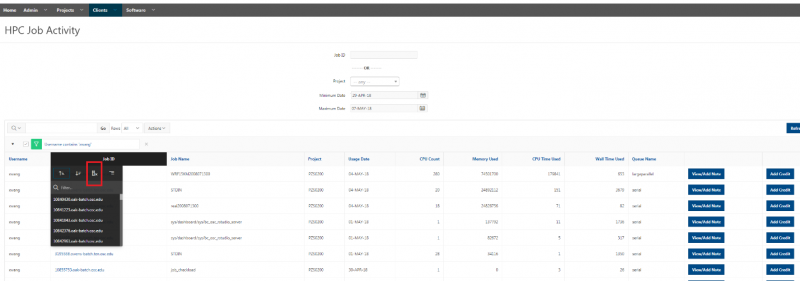
 Map shows that the most expensive segment of the code is lines 83-84 of HPC_sparsemv.cpp:
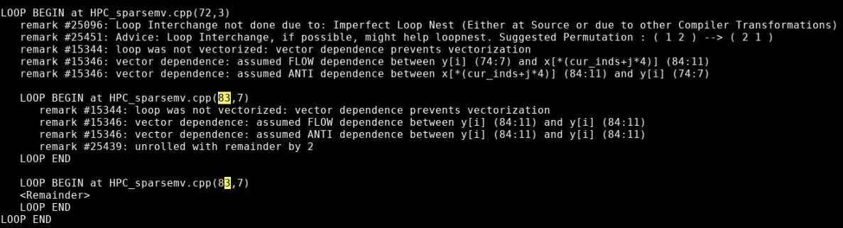


 ":
":


 symbol. Click the