Table of Contents
Introduction
This tutorial presents techniques to tune the performance of an application. Keep in mind that correctness of results, code readability/maintainability, and portability to future systems are more important than performance. For a big picture view, you can check the status of a node while a job is running by visiting the OSC grafana page and using the "cluster metrics" report, and you can use the online interactive tool XDMoD to look at resource usage information for a job.
Some application software specific factors that can affect performance are
- Effective use of processor features for a high degree of internal concurrency in a single core
- Memory access patterns (memory access is slow compared to computation)
- Use of an appropriate file system for file I/O
- Scalability of algorithms
- Compiler optimizations
- Explicit parallelism
We will be using this code based on the HPCCD miniapp from Mantevo. It performs the Conjugate Gradient (CG) on a 3D chimney domain. CG is an iterative algorithm to numerically approximate the solution to a system of linear equations.
Run code with:
srun -n <numprocs> ./test_HPCCG nx ny nz
where nx, ny, nz are the number of nodes in the x, y, and z dimension on each processor.
Setup
First start an interactive Pitzer Desktop session with OnDemand.
You need to load intel 19.0.5 and mvapich2 2.3.3:
module load intel/19.0.5 mvapich2/2.3.3
Then clone the repository:
git clone https://code.osu.edu/khuvis.1/performance_handson.git
Debugging
Debuggers let you execute your program one line at a time, inspect variable values, stop your programming at a particular line, and open a core file after the program crashes.
For debugging, use the -g flag and remove optimzation or set to -O0. For example:
icc -g -o mycode.c
gcc -g -O0 -o mycode mycode.c
To see compiler warnings and diagnostic options:
icc -help diag
man gcc
ARM DDT
ARM DDT is a commercial debugger produced by ARM. It can be loaded on all OSC clusters:
module load arm-ddt
To run a non-MPI program from the command line:
ddt --offline --no-mpi ./mycode [args]
To run an MPI program from the command line:
ddt --offline -np num.procs ./mycode [args]
Hands On
Compile and run the code:
make
srun -n 2 ./test_HPCCG 150 150 150
You should have received the following error message at the end of the program output:
===================================================================================
=   BAD TERMINATION OF ONE OF YOUR APPLICATION PROCESSES
=   PID 308893 RUNNING AT p0200
=   EXIT CODE: 11
=   CLEANING UP REMAINING PROCESSES
=   YOU CAN IGNORE THE BELOW CLEANUP MESSAGES
===================================================================================
YOUR APPPLICATIN TERMINATED WITH EXIT STRING: Segmentation fault (signal 11)
This typically referes to a problem with your application.
Please see tthe FAQ page for debugging suggestions
Set compiler flags -O0 -g to CPP_OPT_FLAGS in Makefile. Then recompile and run with ARM DDT:
make clean; make
module load arm-ddt
ddt -np 2 ./test_HPCCG 150 150 150
Solution
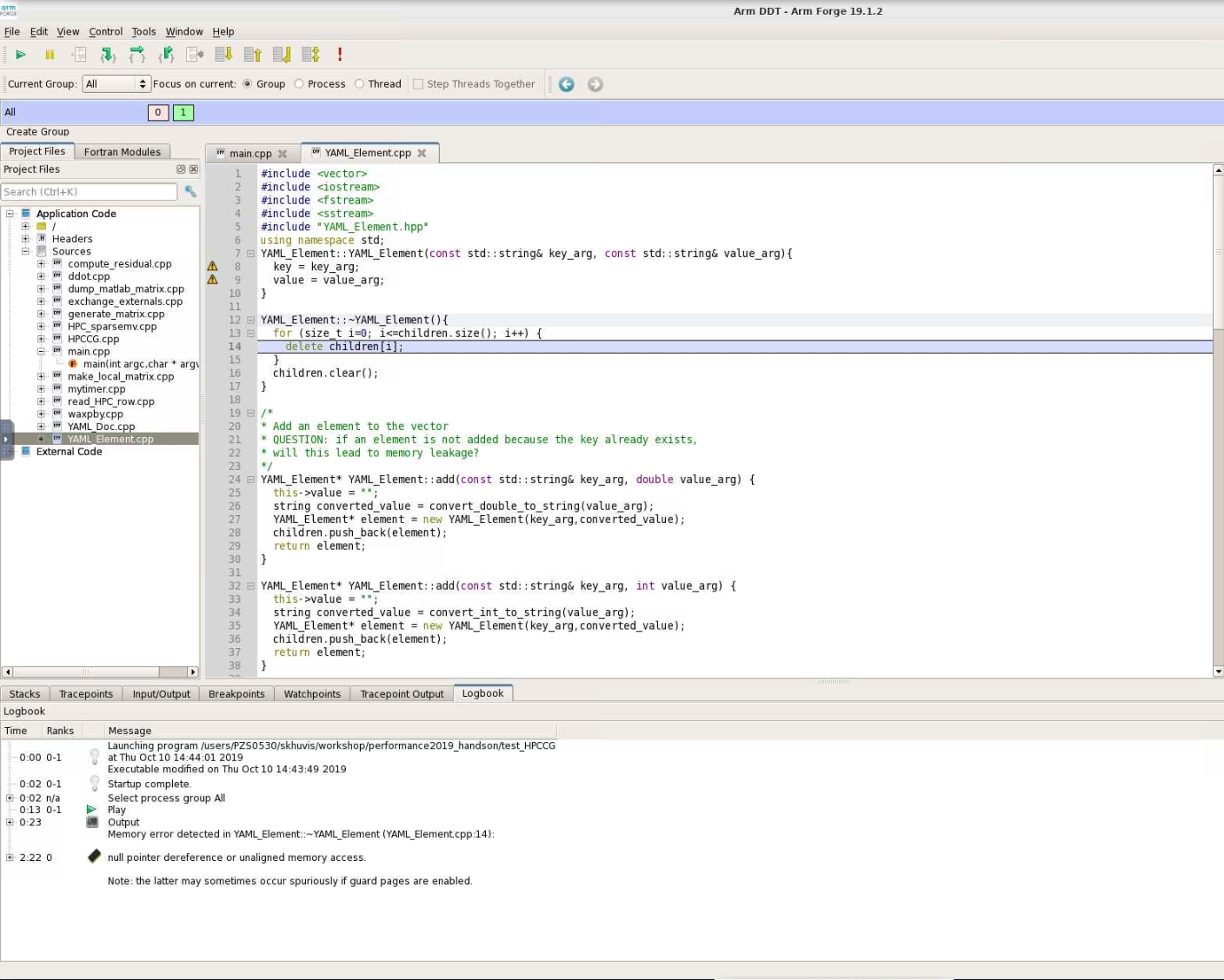
When DDT stops on the segmentation fault, the stack is in the YAML_Element::~YAML_Element function of YAML_Element.cpp. Looking at this function, we see that the loop stops at children.size() instead of children.size()-1. So, line 13 should be changed from
for(size_t i=0; i<=children.size(); i++) {
to
for(size_t i=0; i<children.size(); i++) {
Hardware
On Pitzer, there are 40 cores per node (20 cores per socket and 2 sockets per node). There is support for AVX512, vector length 8 double or 16 single precision values and fused multiply-add. (There is hardware support for 4 thread per core, but it is currently not enabled on OSC systems.)
There are three cache levels on Pitzer, and the statistics are shown in the table below:
| Cache level | Size (KB) | Latency (cycles) | Max BW (bytes/cycle) | Sustained BW (bytes/cycle) |
|---|---|---|---|---|
| L1 DCU | 32 | 4-6 | 192 | 133 |
| L2 MLC | 1024 | 14 | 64 | 52 |
| L3 LLC | 28160 | 50-70 | 16 | 15 |
Never do heavy I/O in your home directory. Home directories are for long-term storage, not scratch files.
One option for I/O intensive jobs is to use the local disk on a compute node. Stage files to and from your home directory into $TMPDIR using the pbsdcp command (e.g. pbsdcp file1 file2 $TMPDIR), and execute the program in $TMPDIR.
Another option is to use the scratch file system ($PFSDIR). This is faster than other file systems, good for parallel jobs, and may be faster than local disk.
For more information about OSC's file system, click here.
For example batch scripts showing the use of $TMPDIR and $PFSDIR, click here.
For more information about Pitzer, click here.
Performance Measurement
FLOPS stands for "floating point operations per second." Pitzer has a theoretical maximum of 720 teraflops. With the LINPACK benchmark of solving a dense system of linear equations, 543 teraflops. With the STREAM benchmark, which measures sustainable memory bandwidth and the corresponding computation rate for vector kernels, copy: 299095.01 MB/s, scale: 298741.01 MB/s, add: 331719.18 MB/s, and traid: 331712.19 MB/s. Application performance is typically much less than peak/sustained performance since applications usually do not take full advantage of all hardware features.
Timing
You can time a program using the /usr/bin/time command. It gives results for user time (CPU time spent running your program), system time (CPU time spent by your program in system calls), and elapsed time (wallclock). It also shows % CPU, which is (user + system) / elapsed, as well as memory, pagefault, swap, and I/O statistics.
/usr/bin/time j3
5415.03user 13.75system 1:30:29elapsed 99%CPU \
(0avgtext+0avgdata 0maxresident)k \
0inputs+0outputs (255major+509333minor)pagefaults 0 swaps
You can also time portions of your code:
| C/C++ | Fortran 77/90 | MPI (C/C++/Fortran) | |
|---|---|---|---|
| Wallclock |
time(2), difftime(3), getrusage(2) |
SYSTEM_CLOCK(2) | MPI_Wtime(3) |
| CPU | times(2) | DTIME(3), ETIME(3) | X |
Profiling
A profiler can show you whether code is compute-bound, memory-bound, or communication bound. Also, it shows how well the code uses available resources and how much time is spent in different parts of your code. OSC has the following profiling tools: ARM Performance Reports, ARM MAP, Intel VTune, Intel Trace Analyzer and Collector (ITAC), Intel Advisor, TAU Commander, and HPCToolkit.
For profiling, use the -g flag and specify the same optimization level that you normally would normally use with -On. For example:
icc -g -O3 -o mycode mycode.c
Look for
- Hot spots (where most of the time is spent)
- Excessive number of calls to short functions (use inlining!)
- Memory usage (swapping and thrashing are not allowed at OSC)
- % CPU (low CPU utilization may mean excessive I/O delays).
ARM Performance Reports
ARM PR works on precompiled binaries, so the -g flag is not needed. It gives a summary of your code's performance that you can view with a browser.
For a non-MPI program:
module load arm-pr
perf-report --no-mpi ./mycode [args]
For an MPI program:
module load arm-pr
perf-report --np num_procs ./mycode [args]
ARM MAP
Interpreting this profile requires some expertise. It gives details about your code's performance. You can view and explore the resulting profile using an ARM client.
For a non-MPI program:
module load arm-map
map --no-mpi ./mycode [args]
For an MPI program:
module load arm-pr
map --np num_procs ./mycode [args]
For more information about ARM Tools, view OSC resources or visit ARM's website.
Intel Trace Analyzer and Collector (ITAC)
ITAC is a graphical tool for profiling MPI code (Intel MPI).
To use:
module load intelmpi # then compile (-g) code
mpiexec -trace ./mycode
View and explore the results using a GUI with traceanalyzer:
traceanalyzer <mycode>.stf
Help From the Compiler
HPC software is traditionally written in Fortran or C/C++. OSC supports several compiler families. Intel (icc, icpc, ifort) usually gives fastest code on Intel architecture). Portland Group (PGI - pgcc, pgc++, pgf90) is good for GPU programming, OpenACC. GNU (gcc, g++, gfortran) is open source and universally available.
Compiler options are easy to use and let you control aspects of the optimization. Keep in mind that different compilers have different values for options. For all compilers, any highly optimized builds, such as those employing the options herein, should be thoroughly validated for correctness.
Some examples of optimization include:
- Function inlining (eliminating function calls)
- Interprocedural optimization/analysis (ipo/ipa)
- Loop transformations (unrolling, interchange, splitting, tiling)
- Vectorization (operate on arrays of operands)
- Automatic parallization of loops (very conservative multithreading)
Compiler flags to try first are:
- General optimization flags (-O2, -O3, -fast)
- Fast math
- Interprocedural optimization/analysis
Faster operations are sometimes less accurate. For Intel compilers, fast math is default with -O2 and -O3. If you have a problem, use -fp-model precise. For GNU compilers, precise math is default with -O2 and -O3. If you want faster performance, use -ffast-math.
Inlining is replacing a subroutine or function call with the actual body of the subprogram. It eliminates overhead of calling the subprogram and allows for more loop optimizations. Inlining for one source file is typically automatic with -O2 and -O3.
Optimization Compiler Options
Options for Intel compilers are shown below. Don't use -fast for MPI programs with Intel compilers. Use the same compiler command to link for -ipo with separate compilation. Many other optimization options can be found in the man pages. The recommended options are -O3 -xHost. An example is ifort -O3 program.f90.
| -fast | Common optimizations |
| -On |
Set optimization level (0, 1, 2, 3) |
| -ipo | Interprocedural optimization, multiple files |
| -O3 | Loop transforms |
| -xHost | Use highest instruction set available |
| -parallel | Loop auto-parallelization |
Options for PGI compilers are shown below. Use the same compiler command to link for -Mipa with separate compilation. Many other optimization options can be found in the man pages. The recommended option is -fast. An example is pgf90 -fast program.f90.
| -fast | Common optimizations |
| -On |
Set optimization level (0, 1, 2, 3, 4) |
| -Mipa | Interprocedural optimization |
| -Mconcur | Loop auto-parallelization |
Options for GNU compilers are shown below. Use the same compiler command to link for -Mipa with separate compilation. Many other optimization options can be found in the man pages. The recommended options are -O3 -ffast-math. An example is gfortran -O3 program.f90.
| -On | Set optimization level (0, 1, 2, 3) |
| N/A for separate compilation | Interprocedural optimization |
| -O3 | Loop transforms |
| -ffast-math | Possibly unsafe floating point optimizations |
| -march=native | Use highest instruction set available |
Hands On
Compile and run with different compiler options:
time srun -n 2 ./test_HPCCG 150 150 150
Using the optimal compiler flags, get an overview of the bottlenecks in the code with the ARM performance report:
module load arm-pr
perf-report -np 2 ./test_HPCCG 150 150 150
Solution
On Pitzer, sample times were:
| Compiler Option | Runtime (seconds) |
|---|---|
| -g | 129 |
| -O0 -g | 129 |
| -O1 -g | 74 |
| -O2 -g | 74 |
| -O3 -g |
74 |
The performance report shows that the code is compute-bound.

Compiler Optimization Reports
Compiler optimization reports let you understand how well the compiler is doing at optimizing your code and what parts of your code need work. They are generated at compile time and describe what optimizations were applied at various points in the source code. The report may tell you why optimizations could not be performed.
For Intel compilers, -qopt-report and outputs to a file.
For Portland Group compilers, -Minfo and outputs to stderr.
For GNU compilers, -fopt-info and ouputs to stderr by default.
A sample output is:
LOOP BEGIN at laplace-good.f(10,7)
   remark #15542: loop was not vectorized: inner loop was already vectorized

   LOOP BEGIN at laplace-good.f(11,10)
   <Peeled loop for vectorization>
   LOOP END

   LOOP BEGIN at laplace-good.f(11,10)
      remark #15300: LOOP WAS VECTORIZED
   LOOP END

   LOOP BEGIN at laplace-good.f(11,10)
   <Remainder loop for vectorization>
      remark #15301: REMAINDER LOOP WAS VECTORIZED
   LOOP END

   LOOP BEGIN at laplace-good.f(11,10)
   <Remainder loop for vectorization>
   LOOP END
LOOP END
Hands On
Add the compiler flag -qopt-report=5 and recompile to view an optimization report.
Vectorization/Streaming
Code is structured to operate on arrays of operands. Vector instructions are built into the processor. On Pitzer, the vector length is 16 single or 8 double precision. The following is a vectorizable loop:
do i = 1,N
  a(i) = b(i) + x(1) * c(i)
end do
Some things that can inhibit vectorization are:
- Loops being in the wrong order (usually fixed by compiler)
- Loops over derived types
- Function calls (can sometimes be fixed by inlining)
- Too many conditionals
- Indexed array accesses
Hands On
Use ARM MAP to identify the most expensive parts of the code.
module load arm-map
map -np 2 ./test_HPCCG 150 150 150
Check the optimization report previously generated by the compiler (with -qopt-report=5) to see if any of the loops in the regions of the code are not being vectorized. Modify the code to enable vectorization and rerun the code.
Solution
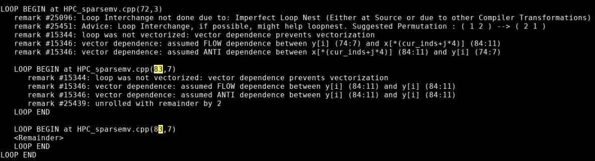
 Map shows that the most expensive segment of the code is lines 83-84 of HPC_sparsemv.cpp:
for (int j=0; j< cur_nnz; j++)
  y[i] += cur_vals[j]*x[cur_inds[j]];
The optimization report confirms that the loop was not vectorized due to a dependence on y.
Incrementing a temporary variable instead of y[i], should enable vectorization:
for (int j=0; j< cur_nnz; j++)
  sum += cur_vals[j]*x[cur_inds[j]];
y[i] = sum;
Recompiling and rerunning with change reduces runtime from 74 seconds to 63 seconds.
Memory access is often the most important factor in your code's performance. Loops that work with arrays should use a stride of one whenever possible. C and C++ are row-major (store elements consecutively by row in 2D arrays), so the first array index should be the outermost loop and the last array index should be the innermost loop. Fortran is column-major, so the reverse is true. You can get factor of 3 or 4 speedup just by using unit stride. Avoid using arrays of derived data types, structs, or classes. For example, use structs of arrays instead of arrays of structures.
Efficient cache usage is important. Cache lines are 8 words (64 bytes) of consecutive memory. The entire cache line is loaded when a piece of data is fetched.
The code below is a good example. 2 cache lines are used for every 8 loop iterations, and it is unit stride:
real*8 a(N), b(N)
do i = 1,N
  a(i) = a(i) + b(i)
end do

! 2 cache lines:
! a(1), a(2), a(3) ... a(8)
! b(1), b(2), b(3) ... b(8)
The code below is a bad example. 1 cache line is loaded for each loop iteration, and it is not unit stride:
TYPE :: node
  real*8 a, b, c, d, w, x, y, z
END TYPE node
TYPE(node) :: s(N)
do i = 1, N
  s(i)%a = s(i)%a + s(i)%b
end do

! cache line:
! a(1), b(1), c(1), d(1), w(1), x(1), y(1), z(1)
Hands On
Look again at the most expensive parts of the code using ARM MAP:
module load arm-map
map -np 2 ./test_HPCCG 150 150 150
Look for any inefficient memory access patterns. Modify the code to improve memory access patterns and rerun the code. Do these changes improve performance?
Solution
Lines 110-148 of generate_matrix.cpp are nested loops:
for (int ix=0; ix<nx; ix++) {
  for (int iy=0; iy<ny; iy++) {
    for (int iz=0; iz<nz; iz++) {
      int curlocalrow = iz*nx*ny+iy*nx+ix;
      int currow = start_row+iz*nx*ny+iy*nx+ix;
      int nnzrow = 0;
      (*A)->ptr_to_vals_in_row[curlocalrow] = curvalptr;
      (*A)->ptr_to_inds_in_row[curlocalrow] = curindptr;
      .
      .
      .
    }
  }
}
The arrays are accessed in a manner so that consecutive values of ix are accesssed in order. However, our loops are ordered so that the ix is the outer loop. We can reorder the loops so that ix is iterated in the inner loop:
for (int iz=0; iz<nz; iz++) {
  for (int iy=0; iy<ny; iy++) {
    for (int ix=0; ix<nx; ix++) {
      .
      .
      .
    }
  }
}
This reduces the runtime from 63 seconds to 22 seconds.
OpenMP
OpenMP is a shared-memory, threaded parallel programming model. It is a portable standard with a set of compiler directives and a library of support functions. It is supported in compilers by Intel, Portland Group, GNU, and Cray.
The following are parallel loop execution examples in Fortran and C. The inner loop vectorizes while the outer loop executes on multiple threads:
PROGRAM omploop
INTEGER, PARAMETER :: N = 1000
INTEGER i, j
REAL, DIMENSION(N, N) :: a, b, c, x
... ! Initialize arrays
!$OMP PARALLEL DO
do j = 1, N
  do i = 1, N
    a(i, j) = b(i, j) + x(i, j) * c(i, j)
  end do
end do
!$OMP END PARALLEL DO
END PROGRAM omploop
int main() {
  int N = 1000;
  float *a, *b, *c, *x;
... // Allocate and initialize arrays
#pragma omp parallel for
  for (int i = 0; i < N; i++) {
    for (int j = 0; j < N; j++) {
      a[i*N+j] = b[i*N+j] + x[i*N+j] * c[i*N+j]
    }
  }
}
You can add an option to compile a program with OpenMP.
For Intel compilers, add the -qopenmp option. For example, ifort -qopenmp ompex.f90 -o ompex.
For GNU compilers, add the -fopenmp option. For example, gcc -fopenmp ompex.c -o ompex.
For Portland group compilers, add the -mp option. For example, pgf90 -mp ompex.f90 -o ompex.
To run an OpenMP program, requires multiple processors through Slurm (--N 1 -n 40) and set the OMP_NUM_THREADS environment variable (default is use all available cores). For the best performance, run at most one thread per core.
An example script is:
#!/bin/bash
#SBATCH -J omploop
#SBATCH -N 1
#SBATCH -n 40
#SBATCH -t 1:00

export OMP_NUM_THREADS=40
/usr/bin/time ./omploop
For more information, visit http://www.openmp.org, OpenMP Application Program Interface, and self-paced turorials. OSC will host an XSEDE OpenMP workshop on November 5, 2019.
MPI
MPI stands for message passing interface for when multiple processes run on one or more nodes. MPI has functions for point-to-point communication (e.g. MPI_Send, MPI_Recv). It also provides a number of functions for typical collective communication patterns, including MPI_Bcast (broadcasts value from root process to all other processes), MPI_Reduce (reduces values on all processes to a single value on a root process), MPI_Allreduce (reduces value on all processes to a single value and distributes the result back to all processes), MPI_Gather (gathers together values from a group of processes to a root process), and MPI_Alltoall (sends data from all processes to all processes).
A simple MPI program is:
#include <mpi.h>
#include <stdio.h>

int main(int argc, char *argv[]) {
  int rank, size;
  MPI_INIT(&argc, &argv);
  MPI_Comm_rank(MPI_COMM_WORLD, &rank);
  MPI_COMM_size(MPI_COMM_WORLD, &size);
  printf("Hello from node %d of %d\n", rank size);
  MPI_Finalize();
  return(0);
}
MPI implementations available at OSC are mvapich2, Intel MPI (only for Intel compilers), and OpenMPI.
MPI programs can be compiled with MPI compiler wrappers (mpicc, mpicxx, mpif90). They accept the same arguments as the compilers they wrap. For example, mpicc -o hello hello.c.
MPI programs must run in batch only. Debugging runs may be done with interactive batch jobs. srun automatically determines exectuion nodes from PBS:
#!/bin/bash
#SBATCH -J mpi_hello
#SBATCH -N 2
#SBATCH --ntasks-per-node=40
#SBATCH -t 1:00

cd $PBS_O_WORKDIR
srun ./hello
For more information about MPI, visit MPI Forum and MPI: A Message-Passing Interface Standard. OSC will host an XSEDE MPI workshop on September 3-4, 2019. Self-paced tutorials are available here.
Hands On
Use ITAC to get a timeline of the run of the code.
module load intelmpi
LD_PRELOAD=libVT.so \
mpiexec -trace -np 40 ./test_HPCCG 150 150 150
traceanalyzer <stf_file>
Look at the Event Timeline (under Charts). Do you see any communication patterns that could be replaced by a single MPI command?
Solution
Looking at the Event Timeline, we see that a large part of runtime is spent in the following communication pattern: MPI_Barrier, MPI_Send/MPI_Recv, MPI_Barrier. We also see that during this communication rank 0 is sending data to all other rank. We should be able to replace all of these MPI calls with a single call to MPI_Bcast.
The relavent code is in lines 82-89 of ddot.cpp:
  MPI_Barrier(MPI_COMM_WORLD);
  if(rank == 0) {
    for(int dst_rank=1; dst_rank < size; dst_rank++) {
      MPI_Send(&global_result, 1, MPI_DOUBLE, dst_rank, 1, MPI_COMM_WORLD);
    }
  }
  if(rank != 0) MPI_Recv(&global_result, 1, MPI_DOUBLE, 0, 1, MPI_COMM_WORLD, MPI_STATUS_IGNORE);
  MPI_Barrier(MPI_COMM_WORLD);
and can be replaced with:
MPI_Bcast(&global_result, 1, MPI_DOUBLE, 0, MPI_COMM_WORLD);
Interpreted Languages
Although many of the tools we already mentioned can also be used with interpreted languages, most interpreted languages such as Python and R have their own profiling tools.
Since they are still running on th same hardware, the performance considerations are very similar for interpreted languages as they are for compiled languages:
- Vectorization
- Efficient memory utilization
- Use built-in and library functions where possible
- Use appropriate data structures
- Understand and use best practices for the language
One of Python's most common profiling tools is cProfile. The simplest way to use cProfile is to add several arguments to your Python call so that an ordered list of the time spent in all functions called during executation. For instance, if a program is typically run with the command:
python ./mycode.py
replace that with
python -m cProfile -s time ./mycode.py
Here is a sample output from this profiler:
See Python's documentation for more details on how to use cProfile.
One of the most popular profilers for R is profvis. It is not available by default with R so it will need to be installed locally before its first use and loaded into your environment prior to each use. To profile your code, just put how you would usually call your code as the argument into profvis:
$ R
> install.packages('profvis')
> library('profvis')
> profvis({source('mycode.R')}
Here is a sample output from profvis:

For more information on profvis is available here.
Hands On
Python
First, enter the Python/ subdirectory of the code containing the python script ns.py. Profile this code with cProfile to determine the most expensive functions of the code. Next, rerun and profile with the array as an argument to ns.py. Which versions runs faster? Can you determine why it runs faster?
Solution
Execute the following commands:
python -m cProfile -s time ./ns.py
python -m cProfile -s time ./ns.py array
In the original code, 66 seconds out 68 seconds are spent in presPoissPeriodic. When the array argument is passed, the time spent in this function is approximately 1 second and the total runtime goes down to about 2 seconds.
The speedup comes from the vectorization of the main computation in the body of presPoissPeriodic by replacing nester for loops with a single like operation on arrays.
R
Now, enter the R/ subdirectory of the code containing the R script lu.R. Make sure that you have the R module loaded. First, run the code with profvis without any additional arguments and then again with frmt="matrix".
Which version of the code runs faster? Can you tell why it runs faster based on the profile?
Solution
Runtime for the default version is 28 seconds while the runtime when frmt="matrix" is 20 seconds.
Here is the profile with default arguments: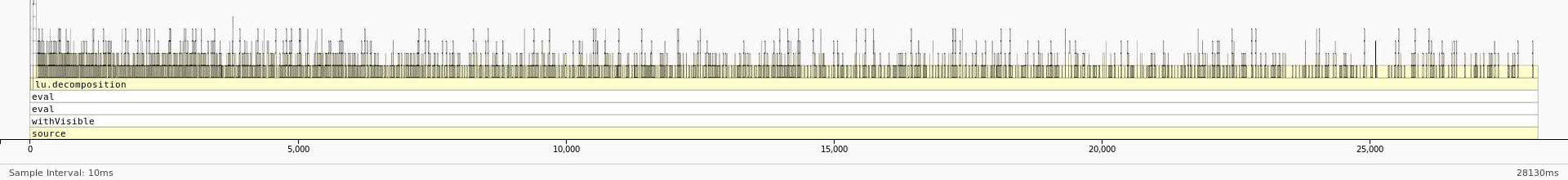
And here is the profile with frmt="matrix":

We can see that most of the time is being spent in lu_decomposition. The difference, however, is that the dataframe version seems to have a much higher overhead associated with accessing elements of the dataframe. On the other hand, the profile of the matrix version seems to be much flatter with fewer functions being called during LU decomposition. This reduction in overhead by using a matrix instead of a dataframe results in the better performance.